
Colorimetric Analysis of Ochratoxin A in Beverage Samples

 ,
,  ,
, 
Abstract
:1. Introduction
2. Materials and Methods
2.1. Solutions and Measurements
- Blank: 1 mL of methanol was mixed with 8 mL of the wine or beer sample and 1 mL of NaHCO3.
- Concentrations: 1 mL of the mix of 8 mL of sample along with 1 mL of 10% NaHCO3 and 1 mL of different previously prepared concentrations of OTA in methanol were mixed to get at final concentration of 2, 5 or 10 ng/mL.
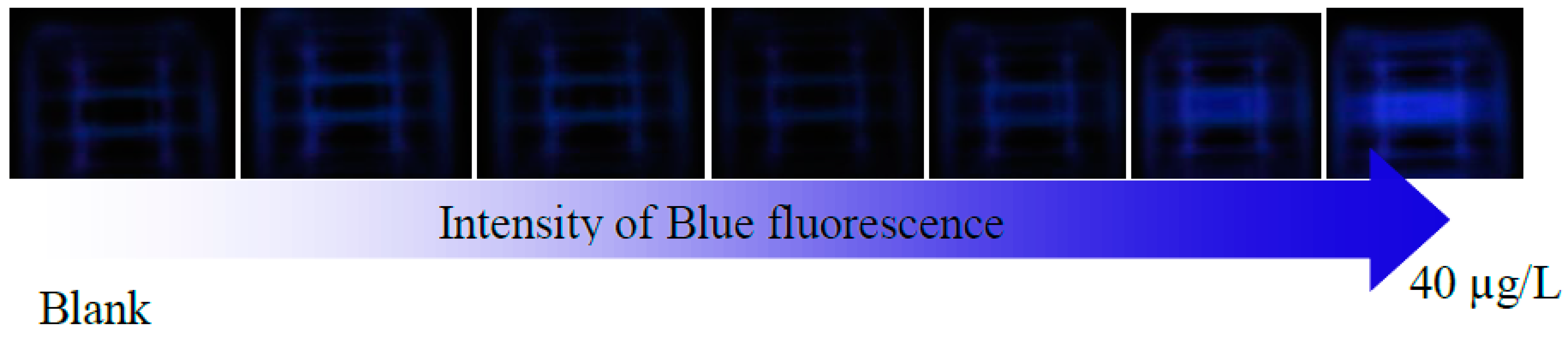
- Measurements: In the device, the samples were excited with UV light, the blank was inserted and three images were taken, the sample was inserted two times more and the image was obtained. Finally, each sample was repeated. The samples of wine and beer were filtered using a 45 µm sterile syringe filter before spiking with OTA. All the measurements were made in triplicate.
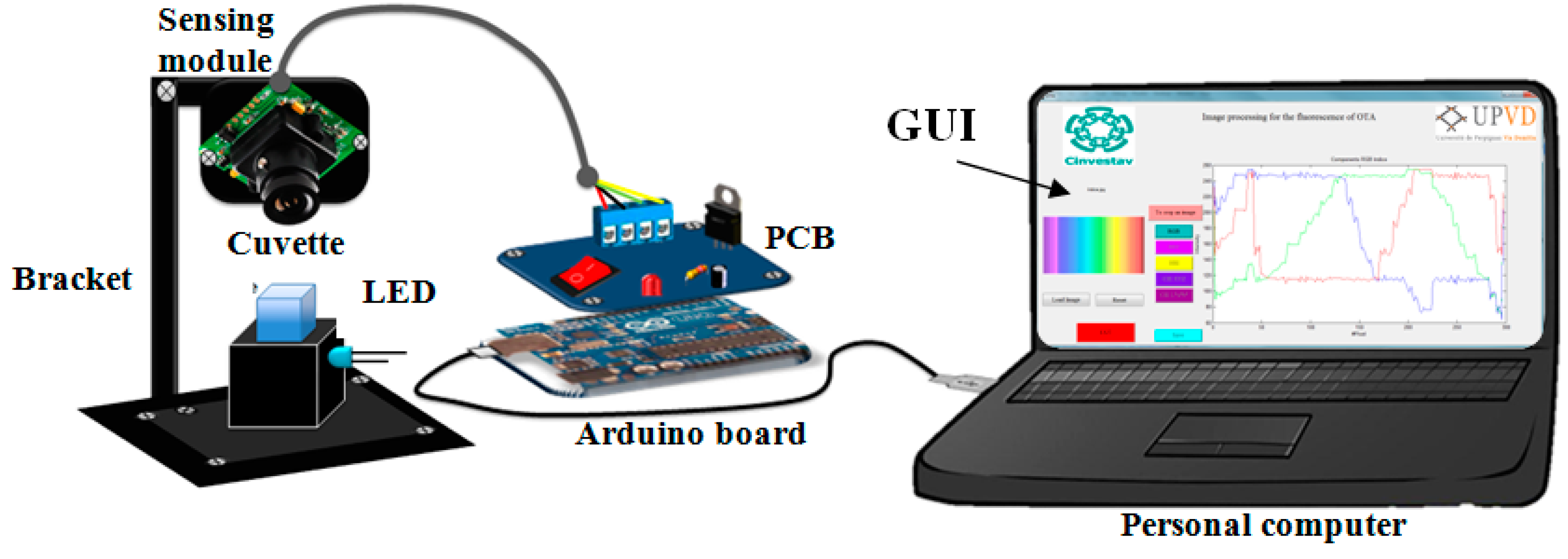
2.2. Instruments
Device Set-up Employed
3. Results and Discussion
3.1. Definition of the Colorimetric Methods Employed
3.1.1. RGB and HSV Models
- H (hue) is the dominant wavelength of the color (red, blue, green).
- S (saturation) is the purity of color (in the sense of the amount of white light mixed with it).
- V (value) is the brightness of the color (also known as luminance).
3.1.2. YCbCr Model
3.1.3. CIEXYZ Model
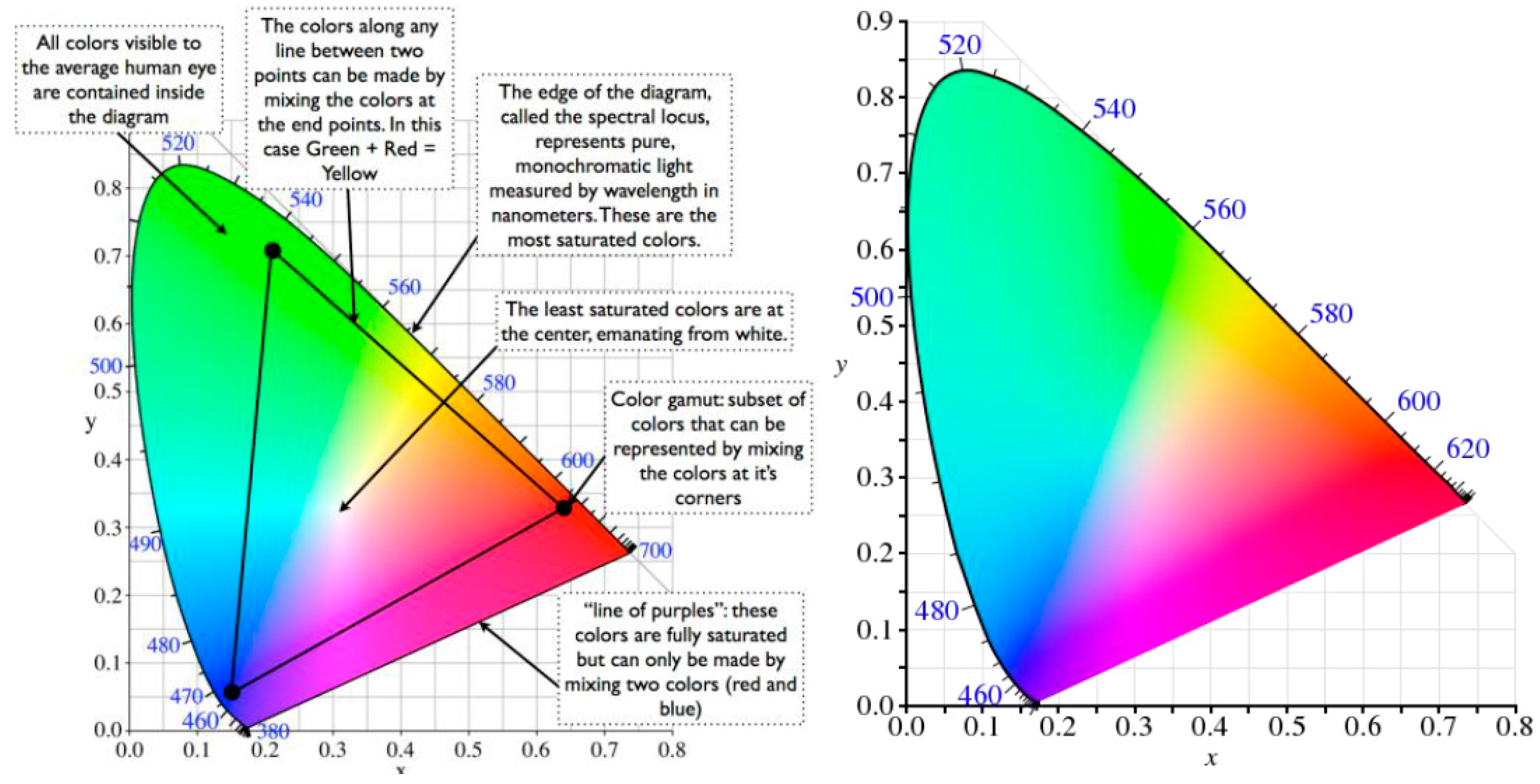
3.1.4. L*a*b* Model
- X, Y and Z are the tristimulus values of the object measured.
- Xn, Yn and Zn are the tristimulus values of a reference white object.
- L* is the visual lightness coordinate.
- a* is the chromatic coordinate ranged approximately from red to green.
- b* is the chromatic coordinate ranged approximately from yellow to blue.
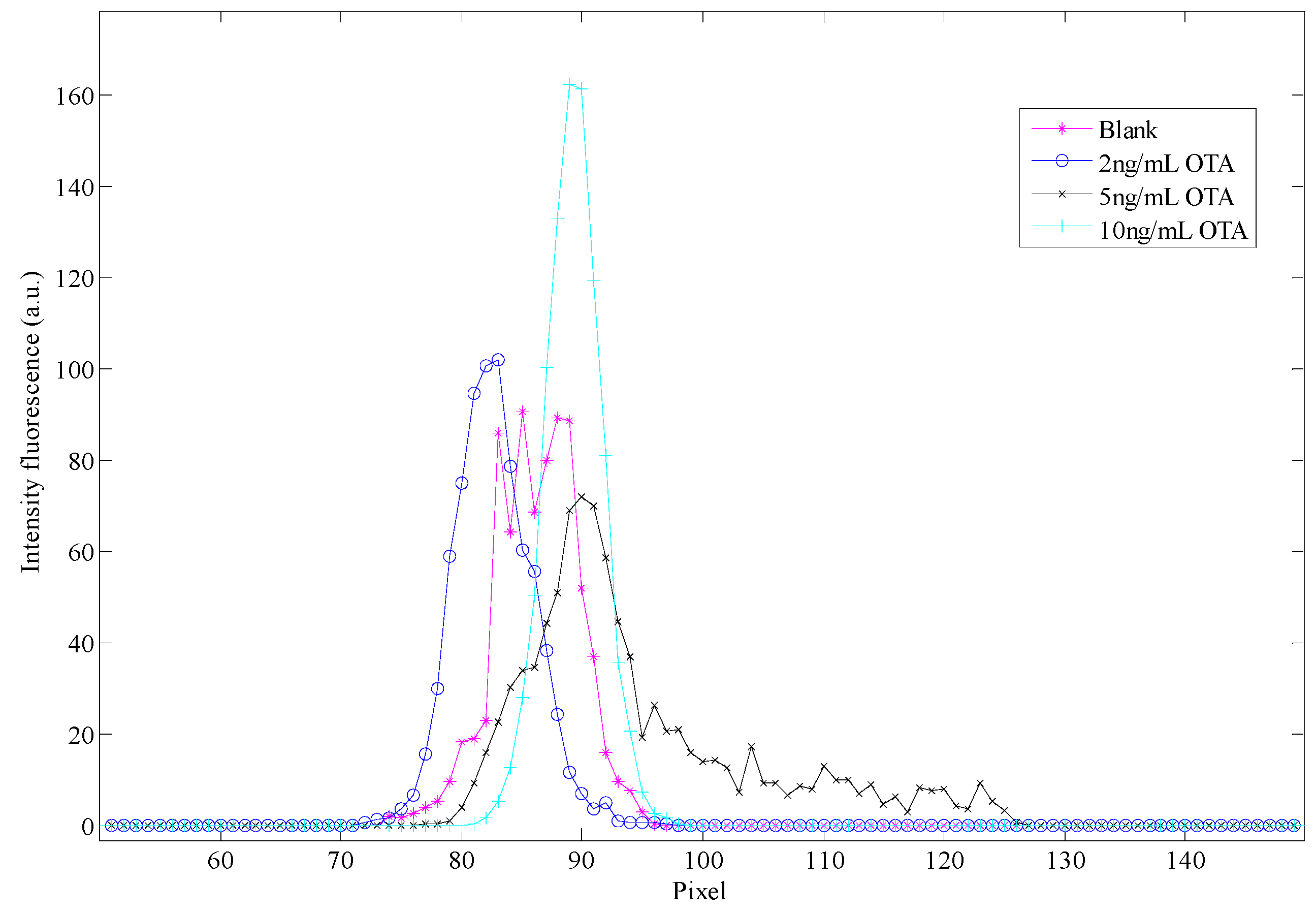
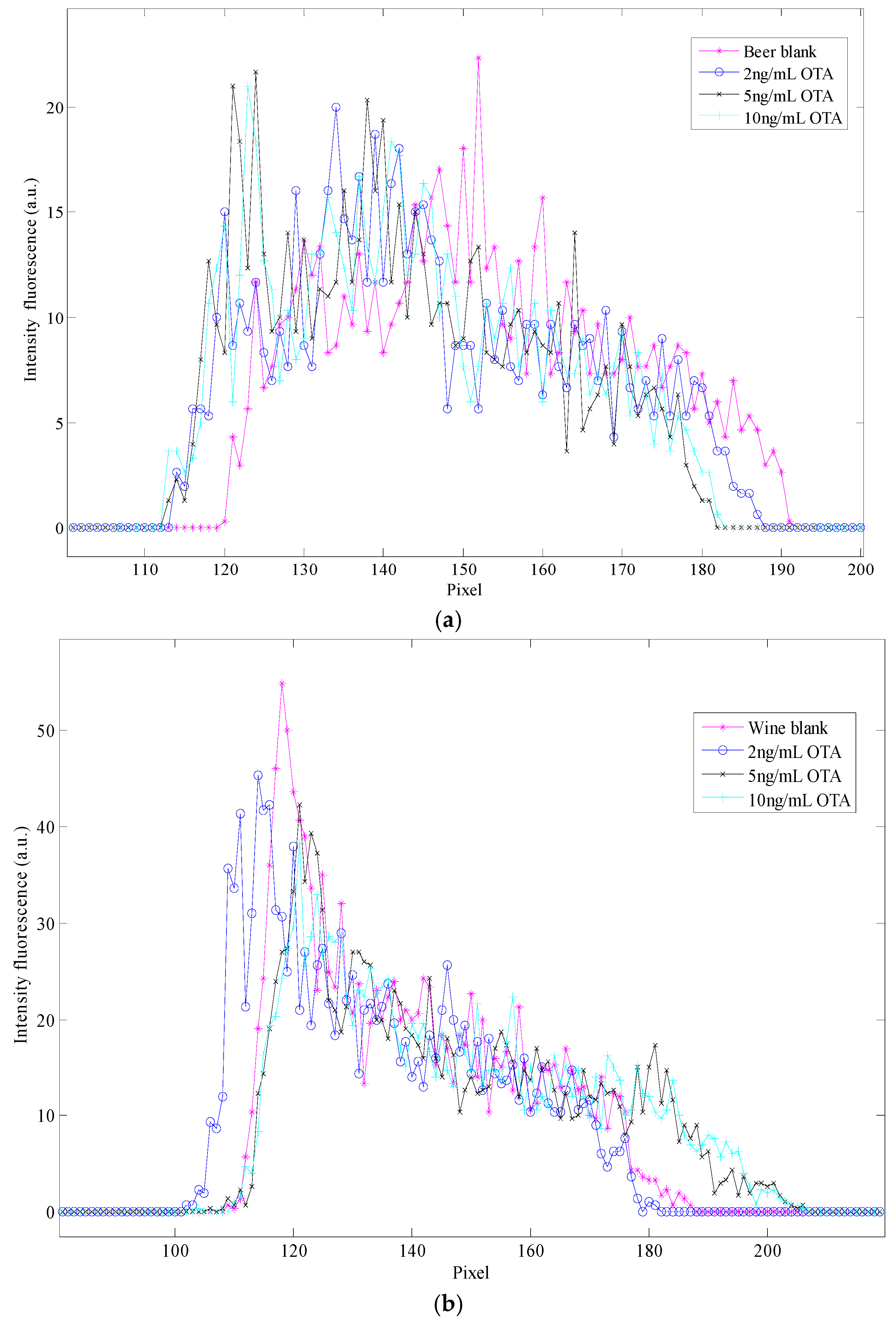
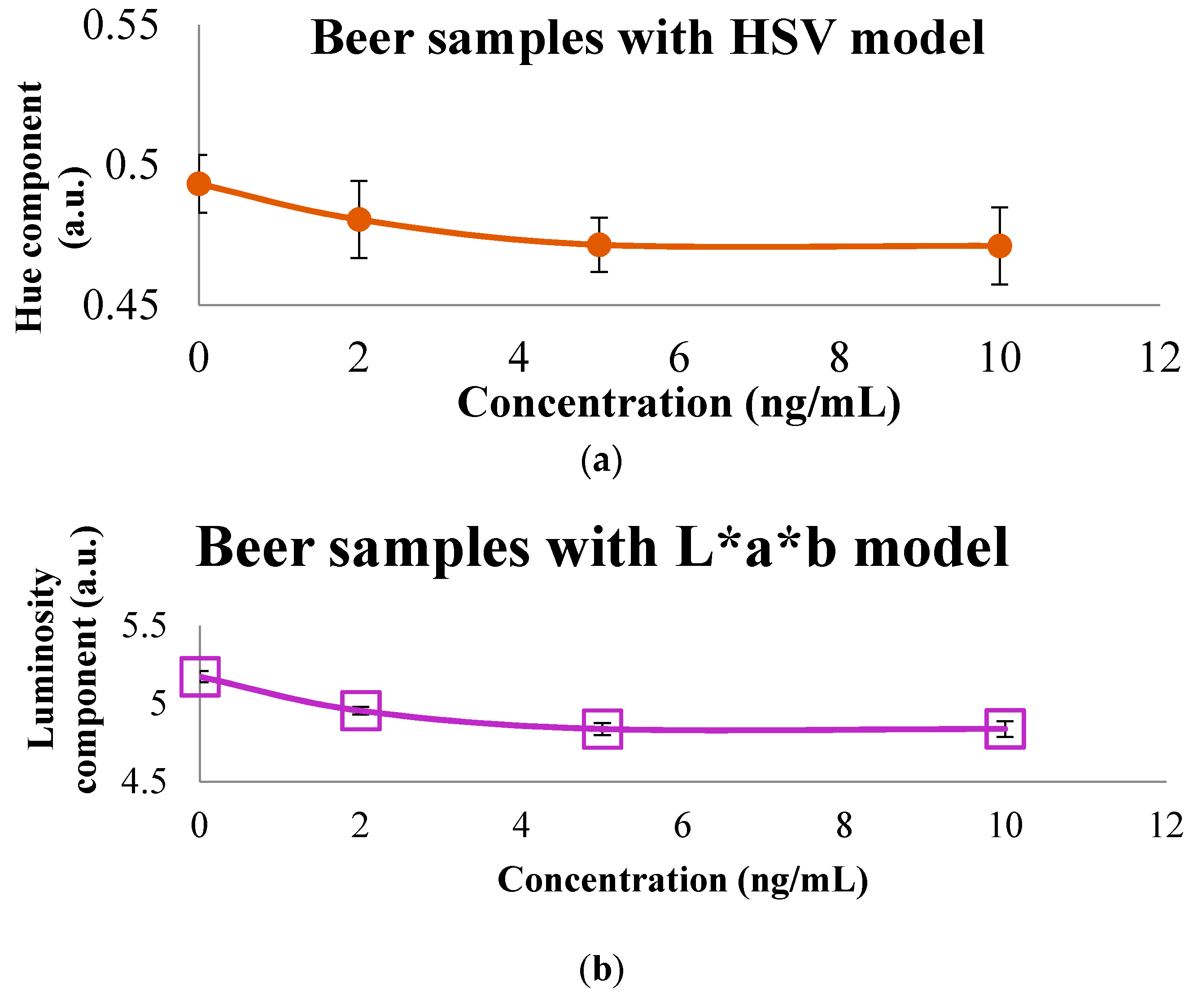
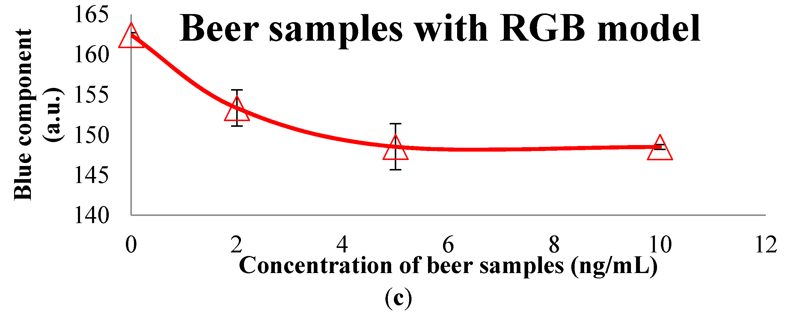
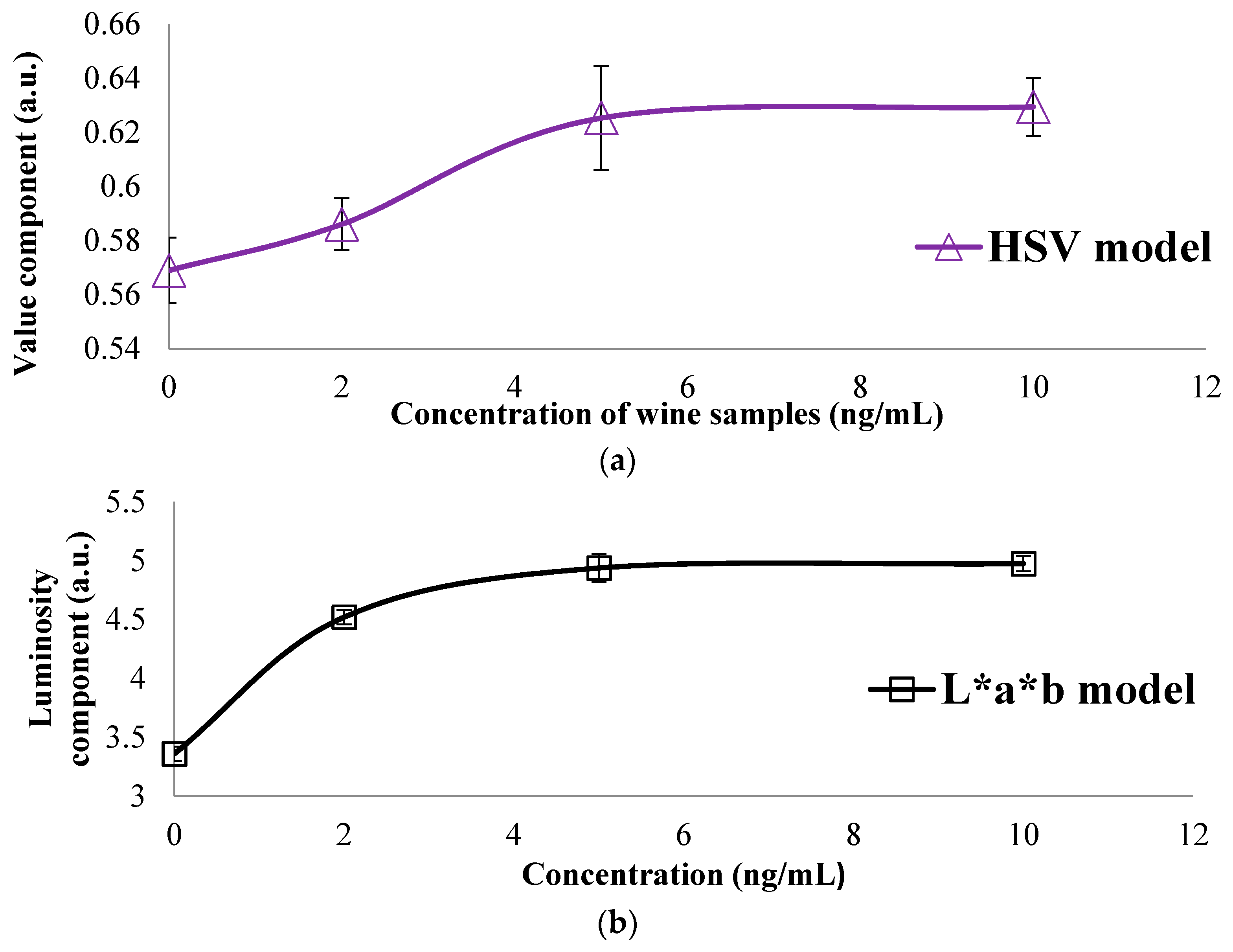
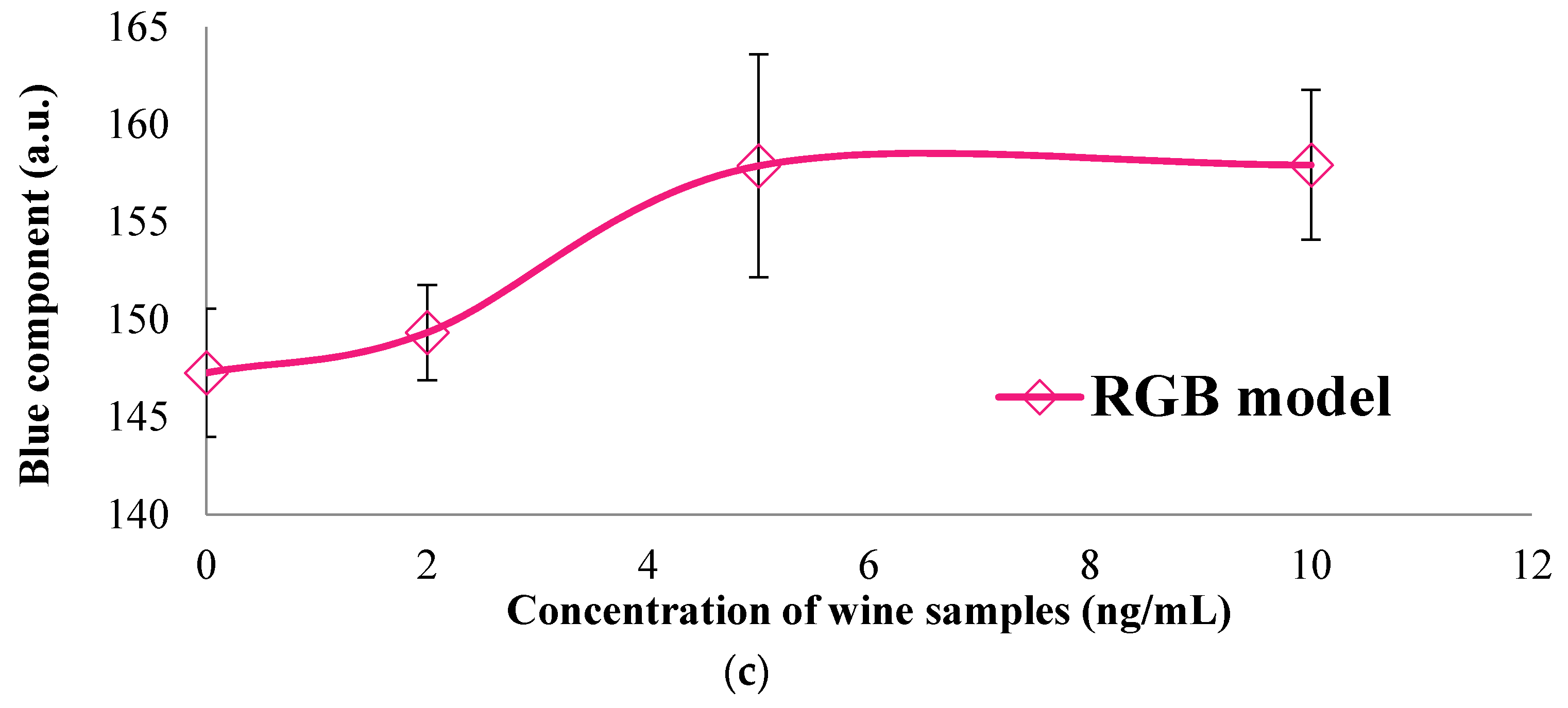
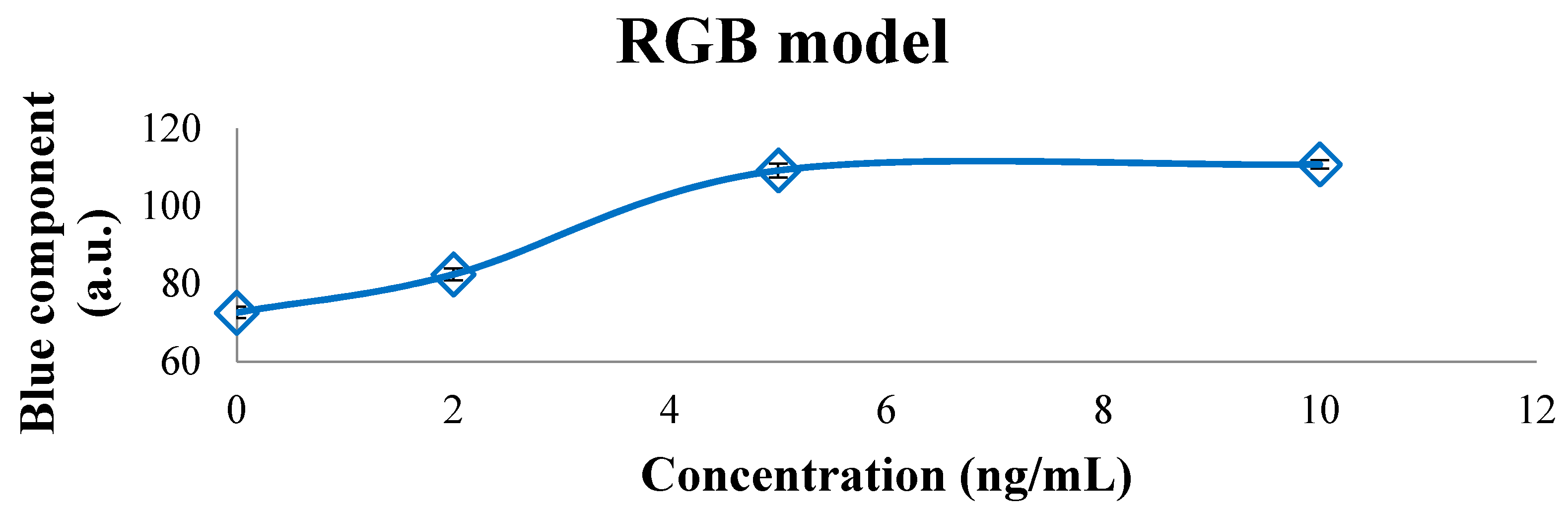
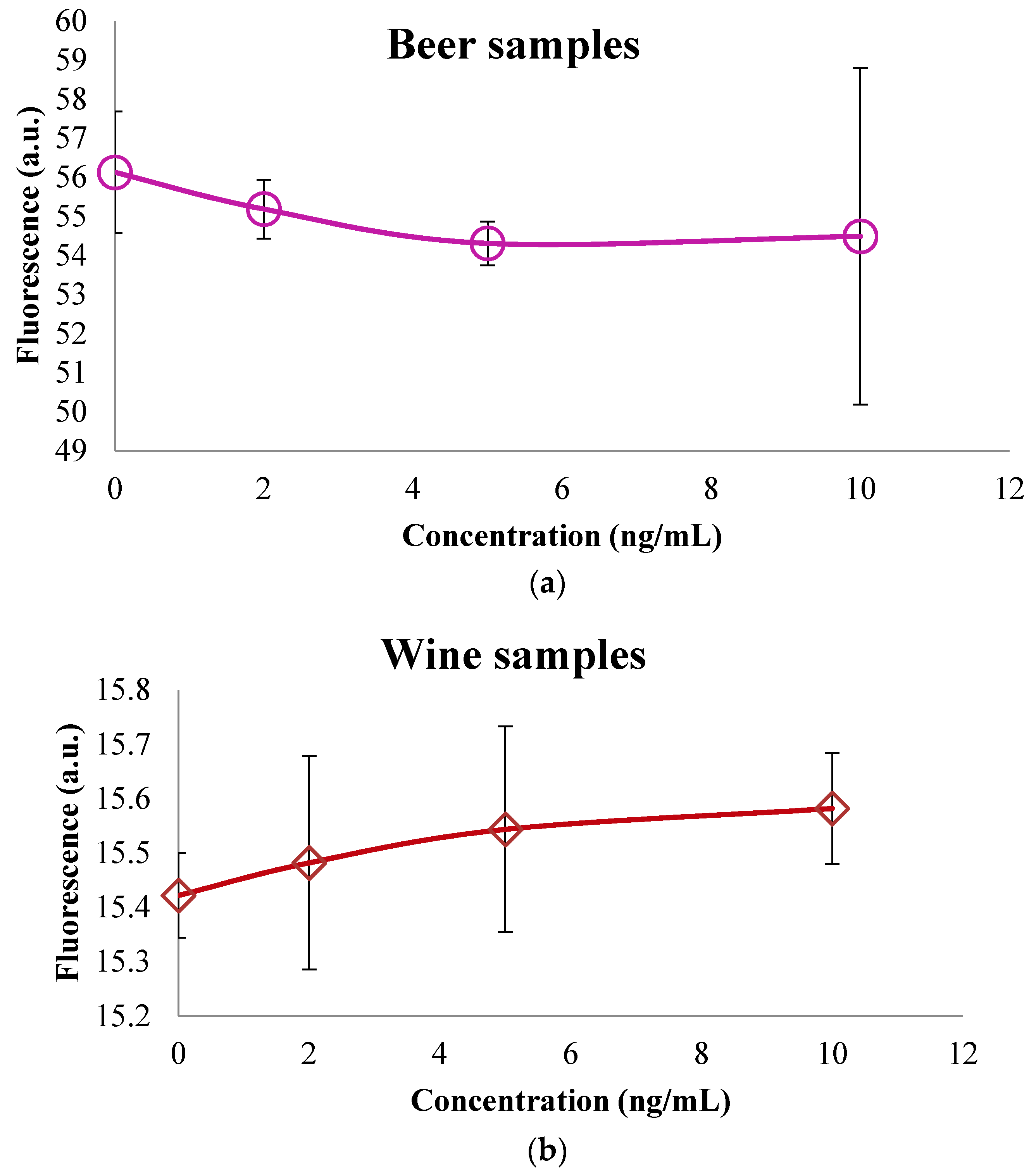
3.2. Colorimetric Methods Applied to Beverage Samples Spiked with OTA
4. Conclusions
Supplementary Materials
Acknowledgments
Author Contributions
Conflicts of Interest
References
- Kostov, Y.; Rao, G. Low-cost optical instrumentation for biomedical measurements. Rev. Sci. Instrum. 2000, 71, 4361–4374. [Google Scholar] [CrossRef]
- Narsaiah, K.; Jha, S.N.; Bhardwaj, R.; Sharma, R.; Kumar, R. Optical biosensors for food quality and safety assurance-A review. J. Food Sci. Technol. 2012, 49, 383–406. [Google Scholar] [CrossRef] [PubMed]
- Committee on Revealing Chemistry trought Advanced Chemical Imaging; Board on Chemical Sciencies and Technology; Division on Earth and Life Studies; National Research Council. Visualizing Chemistry: The Progress and Promise of Advanced Chemical Imaging; National Academies Press: Washington, DC, USA, 2006. [Google Scholar]
- Shyam, N.J. Nondestructive Evaluation of Food Quality, 1st ed.; Springer: Heildelberg, Germany, 2010. [Google Scholar]
- Fernandez Maloigne, C. Advanced Color Image Processing and Analysis, 1st ed.; Springer Science + Business Media: New York, NY, USA, 2013. [Google Scholar]
- León, K.; Mery, D.; Pedreschi, F.; León, J. Color measurement in L∗a∗b∗ units from RGB digital images. Food Res. Int. 2006, 39, 1084–1091. [Google Scholar] [CrossRef]
- Bueno, D.; Muñoz, R.; Marty, J.L. Fluorescence analyzer based on smartphone camera and wireless for detection of Ochratoxin A. Sens. Actuators B Chem. 2016, 232, 462–468. [Google Scholar] [CrossRef]
- Bueno, D.; Mishra, R.K.; Hayat, A.; Catanante, G.; Sharma, V.; Muñoz, R.; Marty, J. Portable and low cost fluorescence set-up for in-situ screnning of Ochratoxin A. Talanta 2016, 159, 395–400. [Google Scholar] [CrossRef] [PubMed]
- Bueno, D.; Istamboulie, G.; Muñoz, R.; Marty, J.L. Determination of Mycotoxins in Food: A Review of Bioanalytical to Analytical Methods. Appl. Spectrosc. Rev. 2015, 50, 728–774. [Google Scholar] [CrossRef]
- Budavari, S. The Merck Index, 11th ed.; Merck & Co.: Rahway, NJ, USA, 1989. [Google Scholar]
- Barug, D.; Bhatnagar, D.; Van Egmond, H.P.; Van Der Kamp, J.W.; Van Osenbruggen, W.A.; Visconti, A. The Mycotoxin Factbook, 1st ed.; Wageningen Academic Publishers: Noordwijk, The Netherlands, 2006. [Google Scholar]
- Murillo-Arbizu, M.T.; Amézqueta, S.; González-Peñas, E.; de Cerain, A.L. Occurrence of ochratoxin a in southern Spanish generous wines under the denomination of origin “Jerez-Xérès-Sherry and ‘Manzanilla’ Sanlúcar de Barrameda”. Toxins 2010, 2, 1054–1064. [Google Scholar] [CrossRef] [PubMed]
- European Commission. Commission Regulation No. 123/2005 of 26 January 2005 amending regulation No. 466/2001 as regards ochratoxin A. Off. J. Eur. Union 2005, L25, 3–5. [Google Scholar]
- Soufleros, E.H.; Tricard, C.; Bouloumpasi, E.C. Occurrence of ochratoxin A in Greek wines. J. Sci. Food Agric. 2003, 83, 173–179. [Google Scholar] [CrossRef]
- Valenta, H. Chromatographic methods for the determination of ochratoxin A in animal and human tissues and fluids. J. Chromatogr. A 1998, 815, 75–92. [Google Scholar] [CrossRef]
- Coskun, A.F.; Wong, J.; Delaram, K.; Nagi, R.; Tey, A.; Ozcan, A. A personalized food allergen testing platform on a cellphone. Lab Chip 2013, 13, 636–640. [Google Scholar] [CrossRef] [PubMed]
- Solomon, C.; Breckon, T. Fundamentals of Digital Image Processing, 1st ed.; Wiley-Blackwell: West Sussex, UK, 2011. [Google Scholar]
- Bueno, D. Optical and Electrochemical Sensing Methods for the Detection of Food Contaminants. Ph.D. Thesis, CINVESTAV-IPN, Mexico City, Mexico, 2016. [Google Scholar]
- Young, I.T.; Gerbrands, J.J.; VanVliet, L.J. Fundamentals of Image Processing, 2nd ed.; Delft University of Technology: Delft, The Netherlands, 1998. [Google Scholar]
- Gonzalez, R.C.; Woods, R.E.; Eddins, S.L. Digital Image Processing Using MATLAB, 2nd ed.; Gatesmark Publishing: Knoxville, TN, USA, 2009. [Google Scholar]
- Cuevas, E.; Zaldivar, D.; Pérez, M. Procesamiento Digital de Imagenes con MATLAB y Simulink, 1st ed.; Alfaomega RA-MA: Madrid, España, 2010. [Google Scholar]
- Plataniotis, K.; Venetsanopoulos, A.N. Color Image Processing and Applications; Springer: Berlin/Heidelberg; New York, NY, USA, 2000. [Google Scholar]
- Wu, Q.; Merchant, F.; Castleman, K. Microscope Image Processing, 1st ed.; Elsevier: San Diego, CA, USA, 2008. [Google Scholar]
- Fairchild, M.D. Color Appearance Models, 3rd ed.; Wiley: Chichester, UK, 2013. [Google Scholar]
- Novo, P.; Moulas, G.; França Prazeres, D.M.; Chu, V.; Conde, J.P. Detection of ochratoxin A in wine and beer by chemiluminescence-based ELISA in microfluidics with integrated photodiodes. Sens. Actuators B Chem. 2013, 176, 232–240. [Google Scholar] [CrossRef]
- Ngundi, M.M.; Shriver-Lake, L.C.; Moore, M.H.; Lassman, M.E.; Ligler, F.S.; Taitt, C.R. Array biosensor for detection of ochratoxin A in cereals and beverages. Anal. Chem. 2005, 77, 148–154. [Google Scholar] [CrossRef] [PubMed]
- Cucci, C.; Mignani, A.G.; Dall’Asta, C.; Pela, R.; Dossena, A. A portable fluorometer for the rapid screening of M1 aflatoxin. Sens. Actuators B Chem. 2007, 126, 467–472. [Google Scholar] [CrossRef]


| Blank | 2 ng/mL | 5 ng/mL | 10 ng/mL | ||
|---|---|---|---|---|---|
| HSV | H | 0.6742 | 0.0000 | 0.6054 | 0.6190 |
| S | 0.1744 | 0.0411 | 0.2056 | 0.2805 | |
| V | 0.3452 | 0.3837 | 0.4281 | 0.4342 | |
| Lab | L | 2.9088 | 2.8184 | 3.2277 | 3.0343 |
| a | −0.6617 | −0.5388 | −0.6525 | −0.5070 | |
| b | 0.3776 | 0.1251 | −0.1919 | −0.3332 | |
| RGB | R | 87.6008 | 80.2075 | 85.6717 | 79.5945 |
| G | 86.4510 | 82.2542 | 95.9654 | 88.3748 | |
| B | 72.5807 | 82.3941 | 109.1670 | 110.7179 | |
| YCbCr | Y | 89.1806 | 86.1331 | 97.0433 | 91.8359 |
| Cb | 121.7540 | 128.3479 | 135.2807 | 138.9271 | |
| Cr | 129.6457 | 126.9936 | 122.4297 | 122.6169 | |
| Blank | 2 ng/mL | 5 ng/mL | 10 ng/mL | ||
|---|---|---|---|---|---|
| HSV | H | 0.4933 | 0.4806 | 0.4716 | 0.4712 |
| S | 0.3059 | 0.2807 | 0.2687 | 0.2774 | |
| V | 0.6565 | 0.6254 | 0.6090 | 0.6140 | |
| Lab | L | 5.1720 | 4.9538 | 4.8370 | 4.8375 |
| a | −1.6932 | −1.5951 | −1.5425 | −1.5571 | |
| b | −0.1835 | −0.1205 | −0.0877 | −0.1052 | |
| RGB | R | 115.7367 | 114.0567 | 112.9867 | 79.5767 |
| G | 167.2433 | 159.4667 | 155.3033 | 156.5533 | |
| B | 162.4400 | 153.3400 | 148.5233 | 148.5036 | |
| YCbCr | Y | 145.9599 | 140.6992 | 137.8622 | 138.5479 |
| Cb | 133.4952 | 131.9739 | 131.2191 | 131.7138 | |
| Cr | 105.7098 | 108.4872 | 109.9113 | 109.0998 |
| Blank | 2 ng/mL | 5 ng/mL | 10 ng/mL | ||
|---|---|---|---|---|---|
| HSV | H | 0.5208 | 0.5226 | 0.5027 | 0.5015 |
| S | 0.2805 | 0.2736 | 0.2859 | 0.2859 | |
| V | 0.5689 | 0.5860 | 0.6252 | 0.6293 | |
| Lab | L | 3.3598 | 4.5206 | 4.9374 | 4.9740 |
| a | −1.3657 | −1.3097 | −1.5539 | −1.5833 | |
| b | −0.2887 | −0.2834 | −0.2229 | −0.1923 | |
| RGB | R | 110.1233 | 107.0967 | 112.6433 | 113.4567 |
| G | 148.5033 | 142.9267 | 158.4767 | 159.9333 | |
| B | 147.2698 | 149.3367 | 157.8900 | 157.8915 | |
| YCbCr | Y | 134.2763 | 130.1840 | 140.2895 | 141.1679 |
| Cb | 136.2398 | 136.0407 | 134.4983 | 133.6966 | |
| Cr | 110.7673 | 111.8285 | 107.8862 | 107.7507 |
| Analytical Features | HPLC | Developed Device | Smartphone as Detector [7] | Amorphous Silicon Photodiode [25] | Array Biosensors (Cereals & Beverage) [26] | Fluorometer for Aflatoxin Detection [27] |
|---|---|---|---|---|---|---|
| LOD (Limit of Detection) | 2 µg/L | 2 µg/L | 2 µg/L | 850 ng/L | Cereals (3.8 to 100 ng/L), coffee 7 ng/L and wine 38 ng/L | <0.025 ng/L |
| Analysis time | 8 min | 1 min | Less than one min | 1–2 min | - | - |
| Dimensions without computer | ≈340 × 400 × 1000 mm3 | ≈145 × 145 × 150 mm3 | ≈115.2 × 58.6 × 9.3 mm3 | ≈6.2 × 12.6 mm2 | - | - |
| Weight | >34 Kg | <1 Kg | 1.4Kg | <1 Kg | - | - |
| Sample reusability | Yes | Noa | Noa | Noa | Noa | No a |
| Purpose | Q | Q or S | Q or S | Q | Q or S | Q or S |
| Portability | No | Yes | Yes | Nob | Yes | Yes |
| Offline data processing | No | Yes | Yes | No | Yes | Yes |
© 2016 by the authors; licensee MDPI, Basel, Switzerland. This article is an open access article distributed under the terms and conditions of the Creative Commons Attribution (CC-BY) license (http://creativecommons.org/licenses/by/4.0/).
Share and Cite
Bueno, D.; Valdez, L.F.; Gutiérrez Salgado, J.M.; Marty, J.L.; Muñoz, R. Colorimetric Analysis of Ochratoxin A in Beverage Samples. Sensors 2016, 16, 1888. https://doi.org/10.3390/s16111888
Bueno D, Valdez LF, Gutiérrez Salgado JM, Marty JL, Muñoz R. Colorimetric Analysis of Ochratoxin A in Beverage Samples. Sensors. 2016; 16(11):1888. https://doi.org/10.3390/s16111888
Chicago/Turabian StyleBueno, Diana, Luis F. Valdez, Juan Manuel Gutiérrez Salgado, Jean Louis Marty, and Roberto Muñoz. 2016. "Colorimetric Analysis of Ochratoxin A in Beverage Samples" Sensors 16, no. 11: 1888. https://doi.org/10.3390/s16111888
APA StyleBueno, D., Valdez, L. F., Gutiérrez Salgado, J. M., Marty, J. L., & Muñoz, R. (2016). Colorimetric Analysis of Ochratoxin A in Beverage Samples. Sensors, 16(11), 1888. https://doi.org/10.3390/s16111888