
An Accurate Projector Calibration Method Based on Polynomial Distortion Representation


Abstract
:1. Introduction
- Photogrammetry will introduce extra errors into the final measurement result of the projection lens.
- The accuracy of the sub-pixel algorithm is limited by the noise, resolution and dynamic range of the camera.
- Due to the defect of the diffusion plate, the reflectogram is not constant at different orientations and positions.
- Although with the similar structure, the conventional distortion parameters for the imaging lens are not suitable for the projection lens, because high optical efficiency and horizontal posture of the projector is the main concern in designing the projection lens. Large residues will be introduced into the final measurement result by using conventional distortion model.
2. Method of Distortion Measurement and Correction
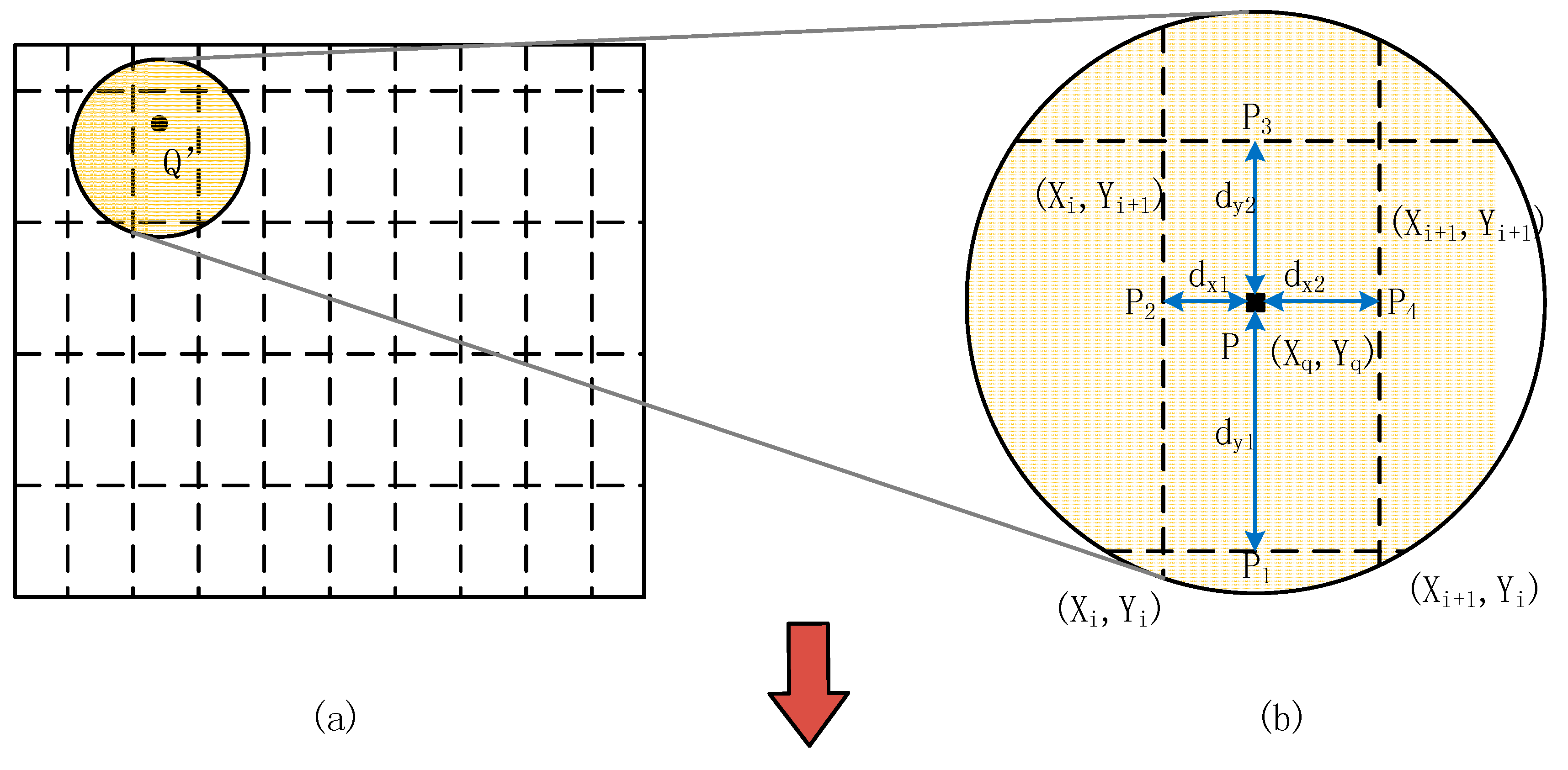
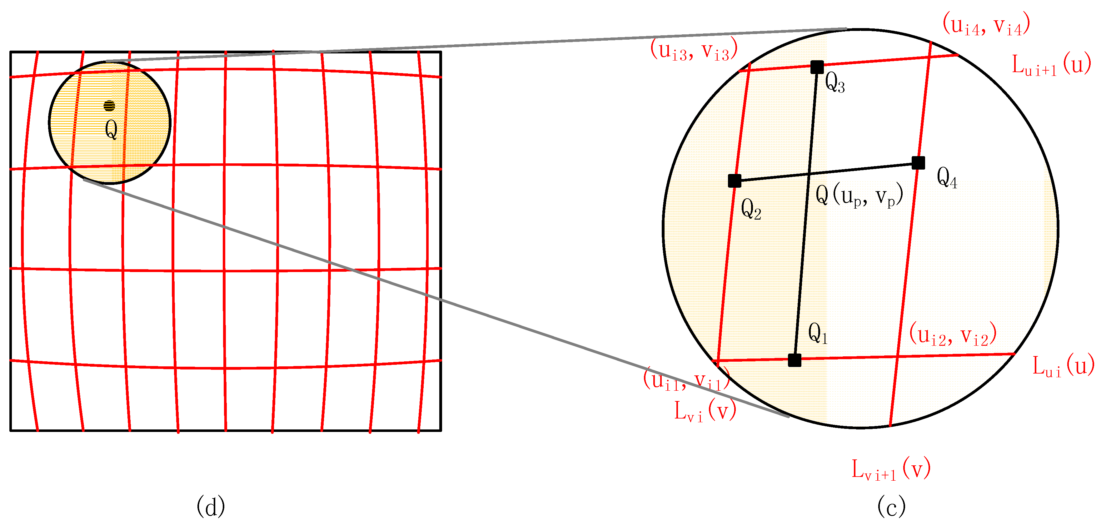
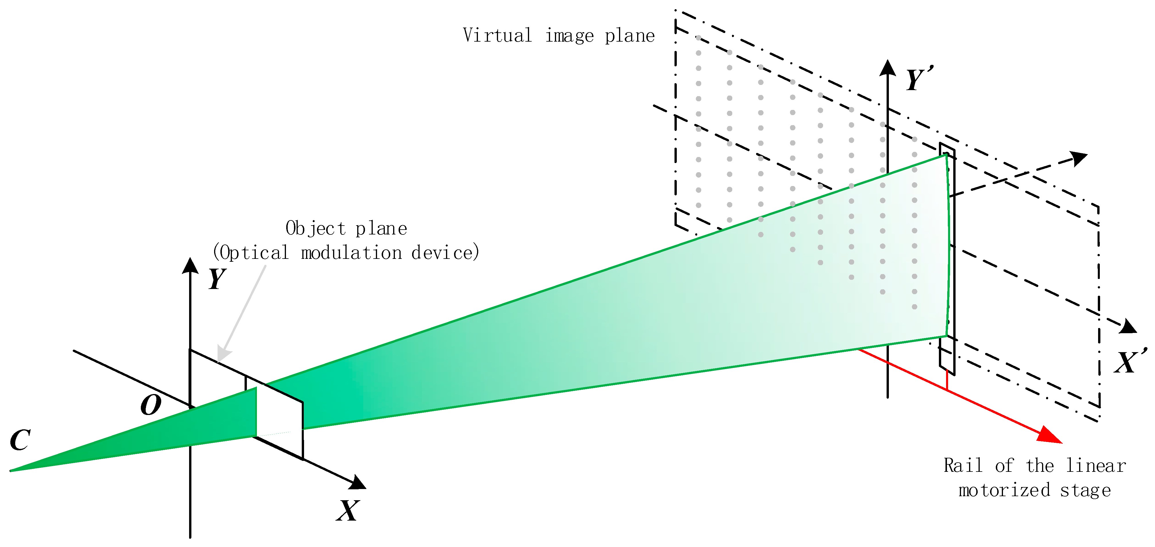
2.1. Principle and Process of Distortion Measurement
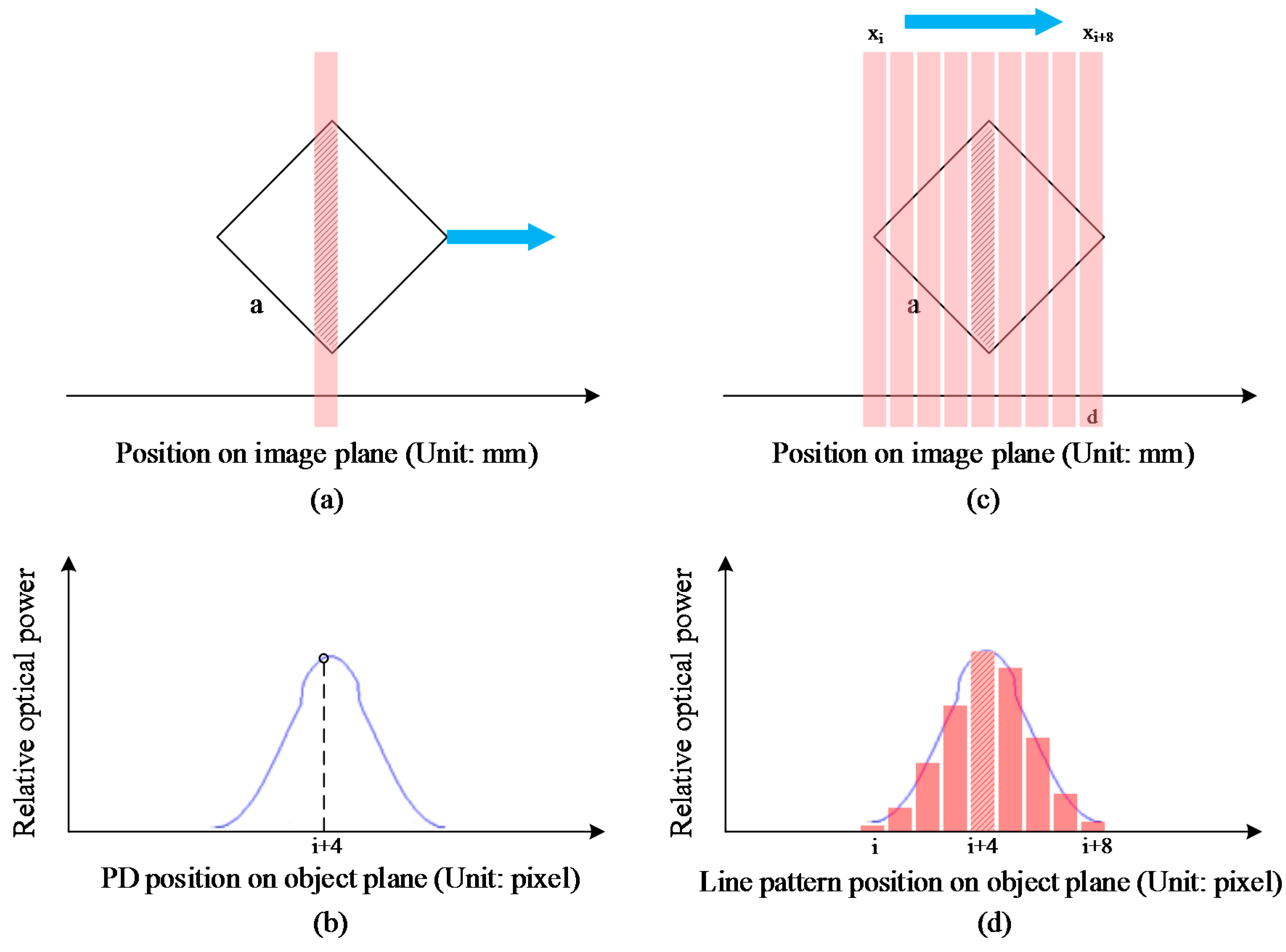
2.2. Subpixel Object Plane Coordinates Extraction of the Corresponding VMPs
2.3. Polynomial Representation of Distortion


2.4. Distortion Correction in Image Space
3. Experiments and Results
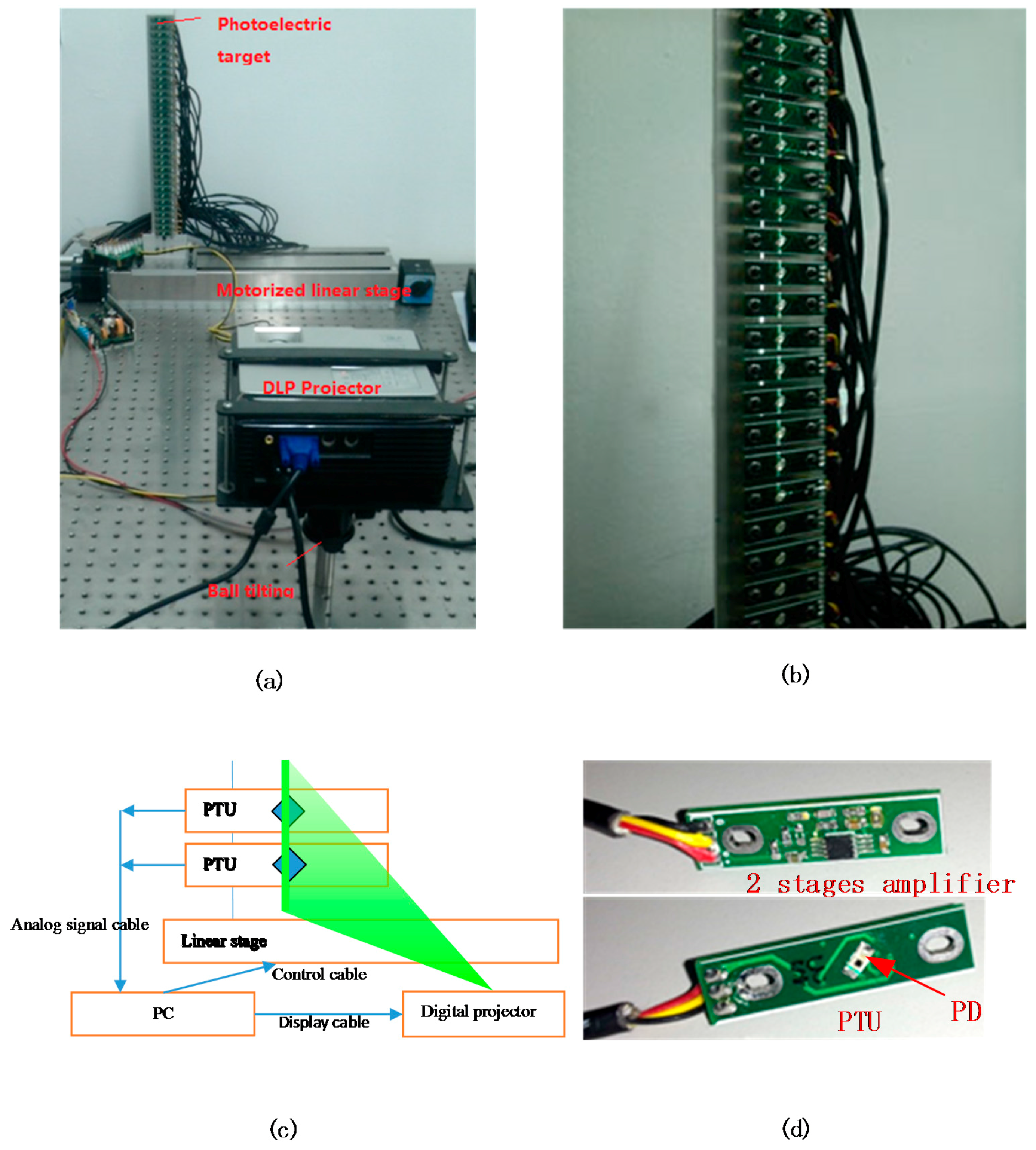
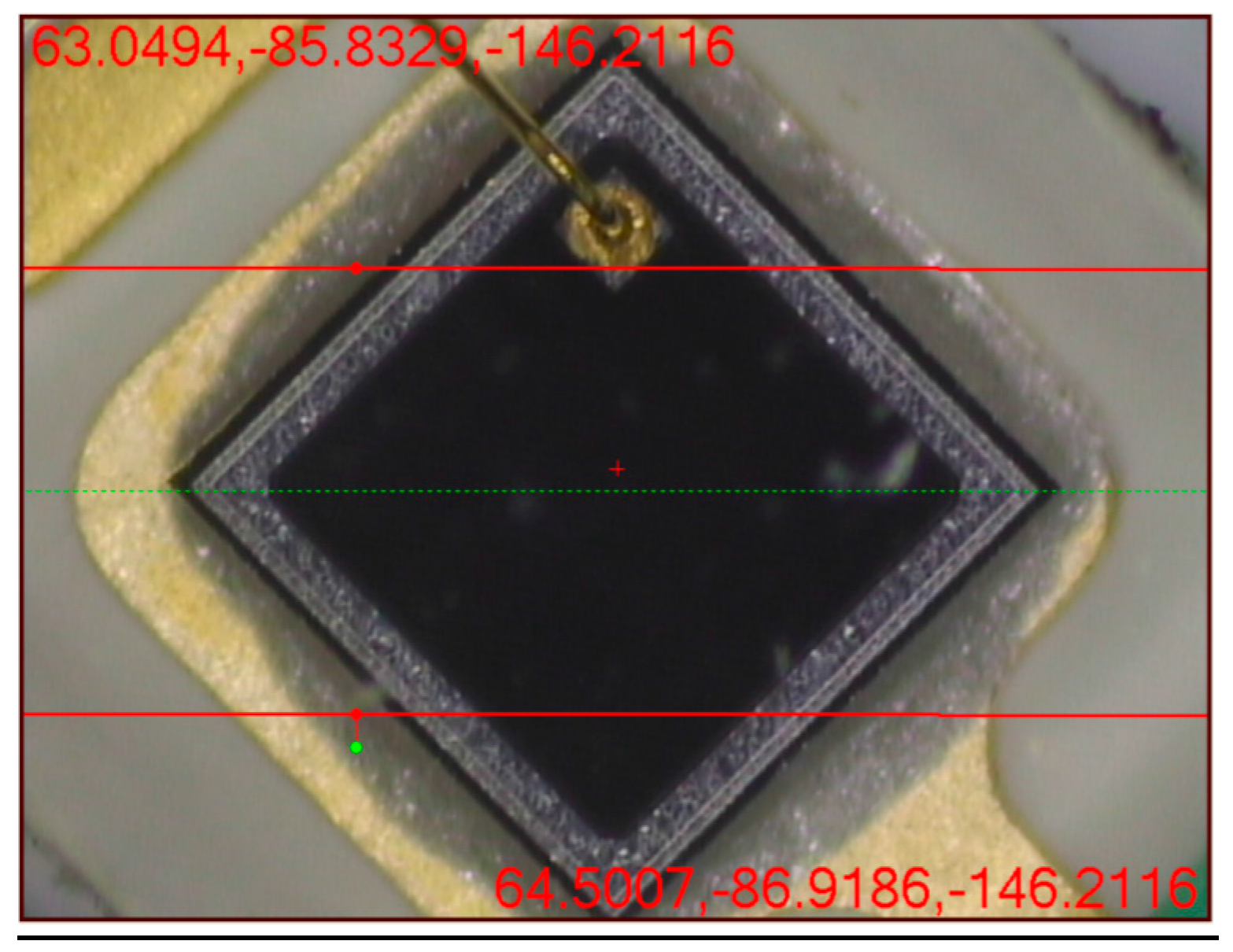
3.1. Experiment Setup

3.2. Measurement Results

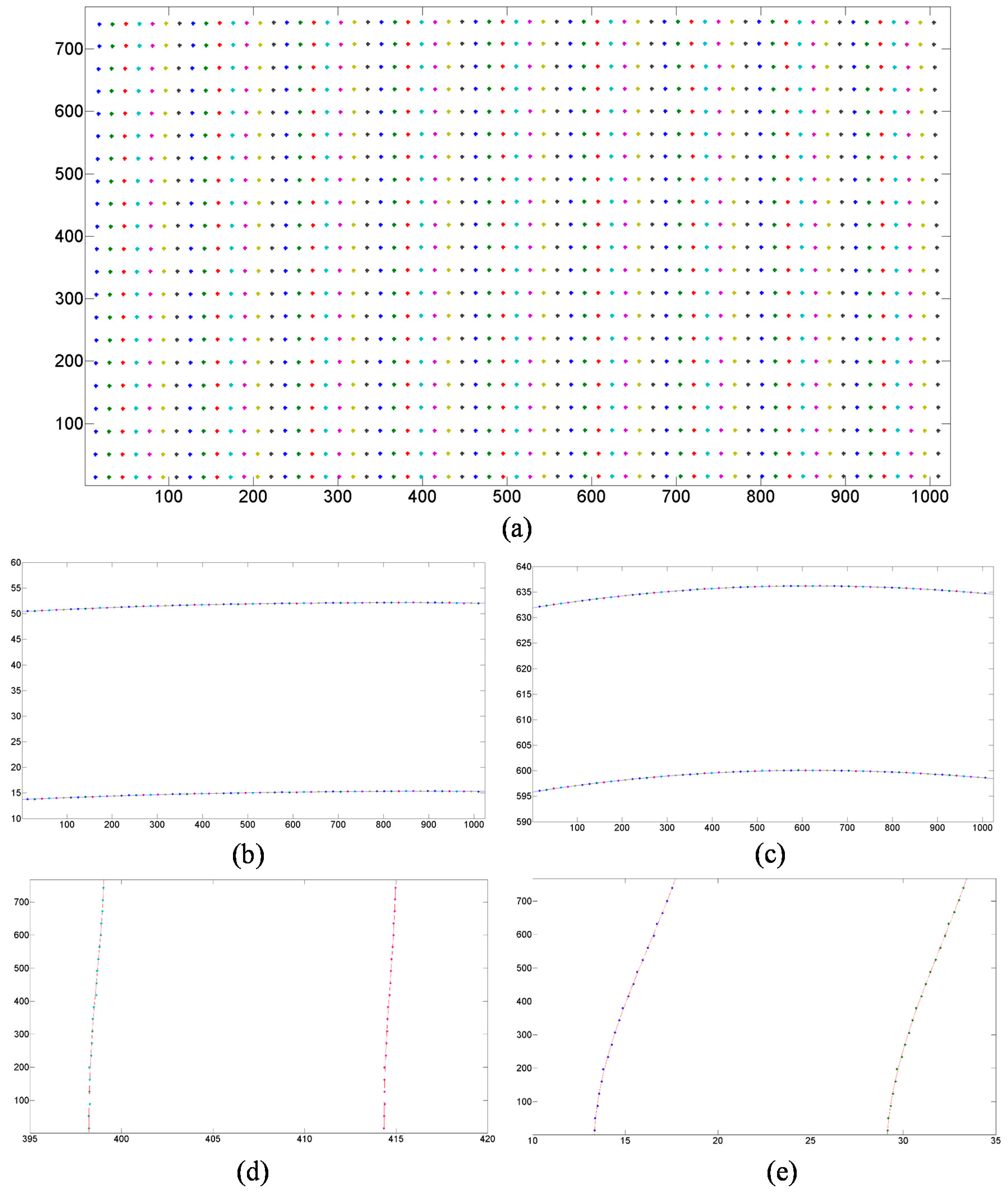
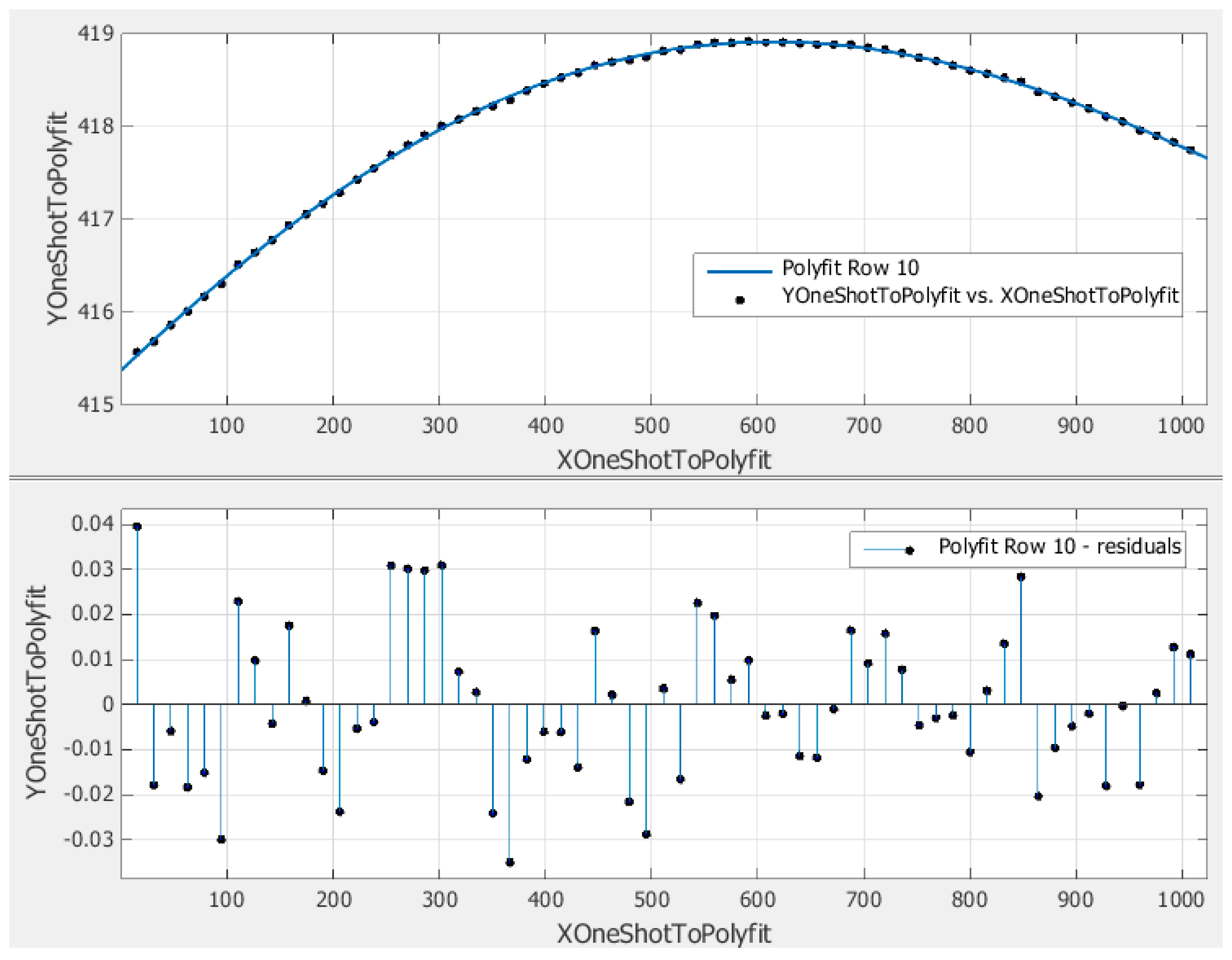
3.3. Quantitative Evaluation
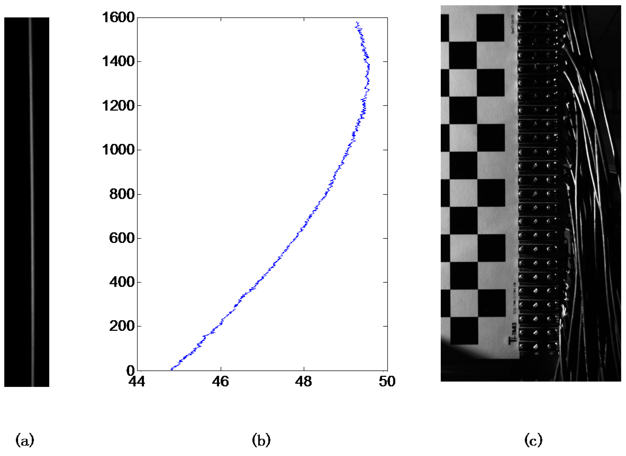
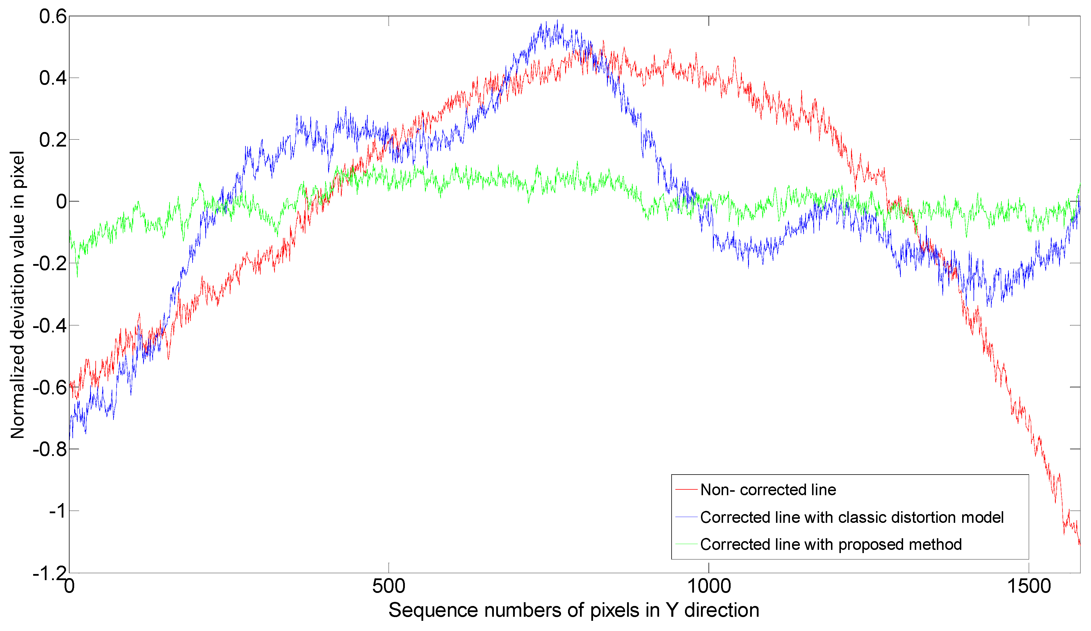
- Uncorrected straight line: Pixel column 17 (Pixel columns are 1–768 from left to right).
- Corrected line by model-based method as shown in Reference [8]: Like the distortion correction of a photograph, the distortion correction of a projector can be achieved by rearranging the pixels on the projector’s object plane with the method based on conventional distortion representation. The ideal line (goal of the correction) on the image plane is the pixel column 17 in the linear (pinhole) model.
- Corrected line by the proposed polynomial distortion representation: The ideal vertical line (goal of the correction) on the image plane is located at 17/768 of the image width.

4. Conclusions
Supplementary Files
Supplementary File 1Acknowledgments
Author Contributions
Conflicts of Interest
References
- Zhang, Z. Review of single-shot 3D shape measurement by phase calculation-based fringe projection techniques. Opt. Lasers Eng. 2012, 50, 1097–1106. [Google Scholar] [CrossRef]
- Cheng, Y.; Li, M.; Lin, J.; Lai, J.; Ke, C.; Huang, Y. Development of dynamic mask photolithography system. In Proceedings of the IEEE International Conference on Mechatronics, Taipei, Taiwan; 2005; pp. 467–471. [Google Scholar]
- Anwar, H.; Din, I.; Park, K. Projector calibration for 3D scanning using virtual target images. Int. J. Precis. Eng. Manuf. 2012, 13, 125–131. [Google Scholar] [CrossRef]
- Huang, Z.; Xi, J.; Yu, Y.; Guo, Q. Accurate projector calibration based on a new point-to-point mapping relationship between the camera and projector images. Appl. Opt. 2015, 54, 347–356. [Google Scholar] [CrossRef]
- Zhang, S.; Huang, P.S. Novel method for structured light system calibration. Opt. Eng. 2006, 45. [Google Scholar] [CrossRef]
- Li, Y.; Shi, S.; Zhong, K.; Wang, C. Projector calibration algorithm for the structured light measurement technique. Acta Opt. Sin. 2009, 11, 3061–3065. [Google Scholar]
- Drareni, J.; Roy, S.; Sturm, P. Geometric video projector auto-calibration. In Proceedings of the IEEE Computer Vision and Pattern Recognition Workshops, Miami, FL, USA; 2009; pp. 39–46. [Google Scholar]
- Xie, L.; Huang, S.; Zhang, Z.; Gao, F.; Jiang, X. Projector calibration method based on optical coaxial camera. In Proceedings of the International Symposium on Optoelectronic Technology and Application 2014: Image Processing and Pattern Recognition, Beijing, China; 2014. [Google Scholar]
- Huang, S.; Xie, L.; Wang, Z.; Zhang, Z.; Gao, F.; Jiang, X. Accurate projector calibration method by using an optical coaxial camera. Appl. Opt. 2015, 54, 789–795. [Google Scholar] [CrossRef] [PubMed]
- Zhang, Z.H.; Huang, S.J.; Meng, S.S.; Gao, F.; Jiang, X.Q. A simple, flexible and automatic 3D calibration method for a phase calculation-based fringe projection imaging system. Opt. Express 2013, 21, 12218–12227. [Google Scholar] [CrossRef] [PubMed]
- Bhasker, E.; Juang, R.; Majumder, A. Registration techniques for using imperfect and partially calibrated devices in planar multi-projector displays. IEEE Trans. Vis. Comput. Gr. 2007, 13, 1368–1375. [Google Scholar] [CrossRef] [PubMed]
- Johnson, T.; Welch, G.; Fuchs, H.; La Force, E.; Towles, H. A distributed cooperative framework for continuous multi-projector pose estimation. In Proceedings of the IEEE Virtual Reality Conference, Lafayette, LA, USA; 2009. [Google Scholar]
- Zhou, J.; Wang, L.; Akbarzadeh, A.; Yang, R. Multi-projector display with continuous self-calibration. In Proceedings of the ACM/IEEE 5th International Workshop on Projector Camera Systems, New York, NY, USA; 2008. [Google Scholar]
- Wang, W.; Zhu, J.; Lin, J. Calibration of a stereoscopic system without traditional distortion models. Opt. Eng. 2013, 52. [Google Scholar] [CrossRef]
- Liu, M.; Yin, S.; Yang, S.; Zhang, Z. An accurate projector gamma correction method for phase-measuring profilometry based on direct optical power detection. In Proceedings of the Applied Optics and Photonics, Beijing, China; 2015. [Google Scholar]
© 2015 by the authors; licensee MDPI, Basel, Switzerland. This article is an open access article distributed under the terms and conditions of the Creative Commons Attribution license (http://creativecommons.org/licenses/by/4.0/).
Share and Cite
Liu, M.; Sun, C.; Huang, S.; Zhang, Z. An Accurate Projector Calibration Method Based on Polynomial Distortion Representation. Sensors 2015, 15, 26567-26582. https://doi.org/10.3390/s151026567
Liu M, Sun C, Huang S, Zhang Z. An Accurate Projector Calibration Method Based on Polynomial Distortion Representation. Sensors. 2015; 15(10):26567-26582. https://doi.org/10.3390/s151026567
Chicago/Turabian StyleLiu, Miao, Changku Sun, Shujun Huang, and Zonghua Zhang. 2015. "An Accurate Projector Calibration Method Based on Polynomial Distortion Representation" Sensors 15, no. 10: 26567-26582. https://doi.org/10.3390/s151026567
APA StyleLiu, M., Sun, C., Huang, S., & Zhang, Z. (2015). An Accurate Projector Calibration Method Based on Polynomial Distortion Representation. Sensors, 15(10), 26567-26582. https://doi.org/10.3390/s151026567