
Balancing Energy Consumption with Hybrid Clustering and Routing Strategy in Wireless Sensor Networks †

Abstract
:1. Introduction
2. Related Works
3. Preliminaries
3.1. Network Model
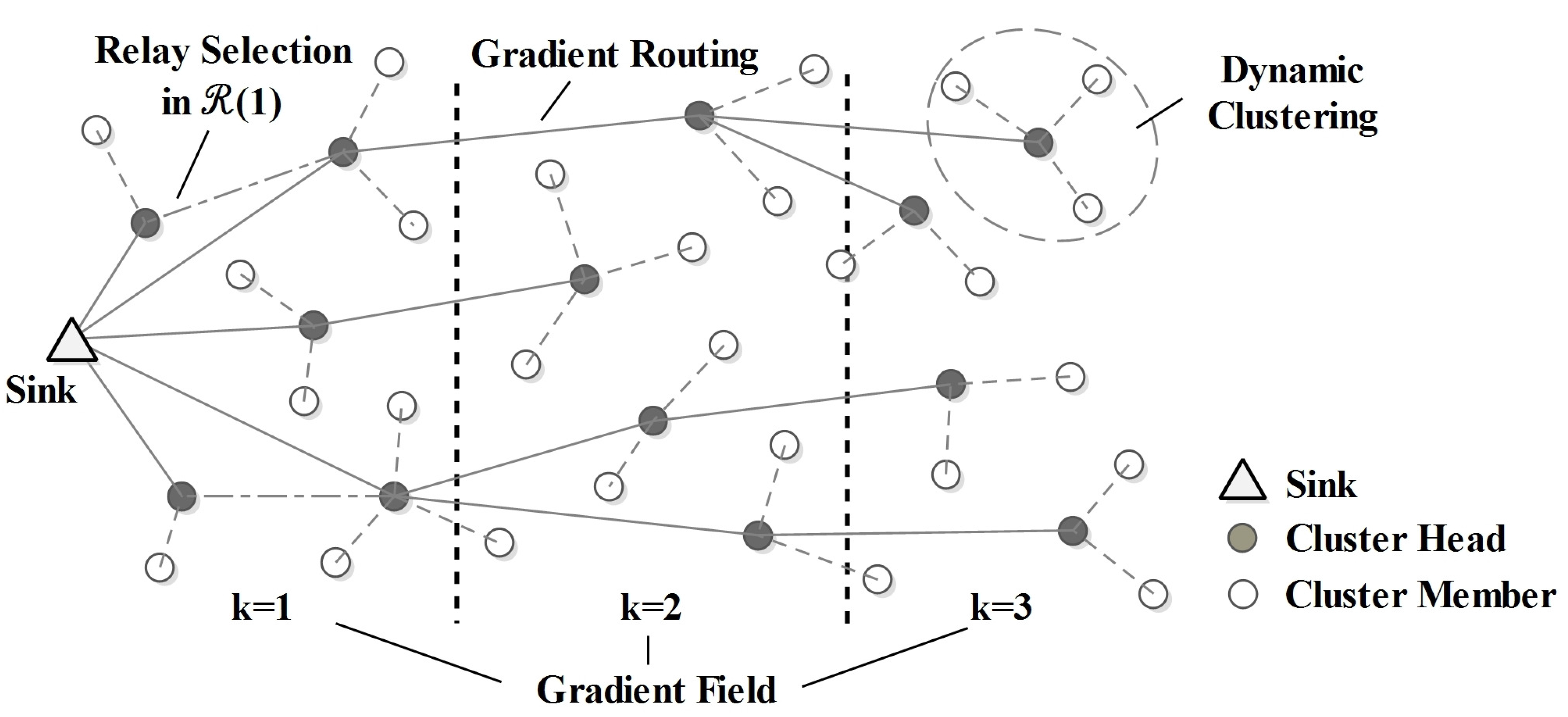
3.2. HCR Protocol
3.2.1. Gradient Field Establishment

| Symbol | Description |
|---|---|
| Clustering range | |
| Inter-cluster transmitting range | |
| N | Number of nodes |
| k | Gradient, which equals the minimum hop count to the sink |
| Ring, the set of nodes with the same gradient j | |
| The estimated distance to the edge of the gradient field | |
| Distance between node i and j | |
| Distance between node i and the sink | |
| Backoff timer | |
| Initial energy of nodes | |
| Residual energy of nodes | |
| Average residual energy of nodes |
3.2.2. Cluster Head Selection
3.2.3. Routing Discovery
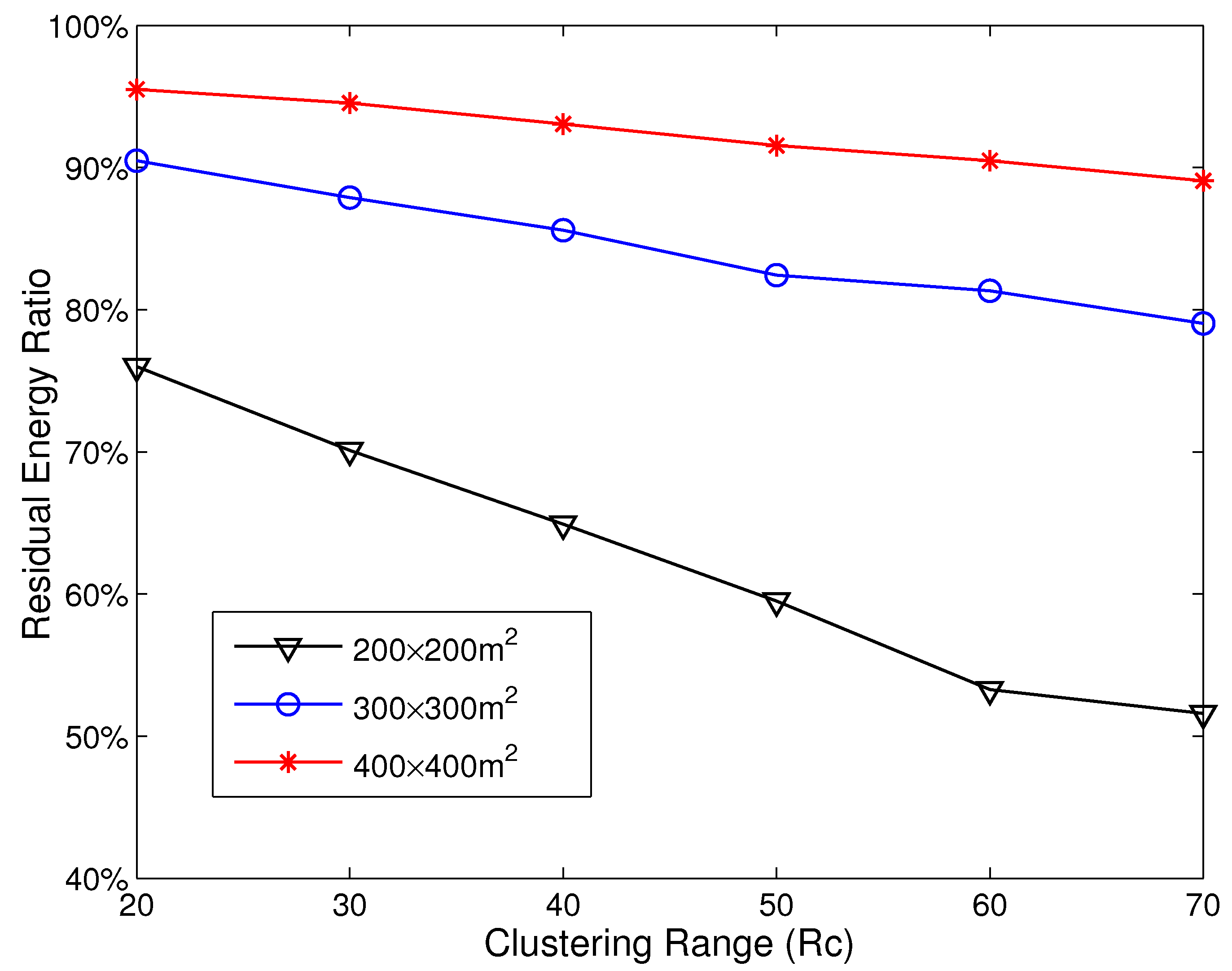
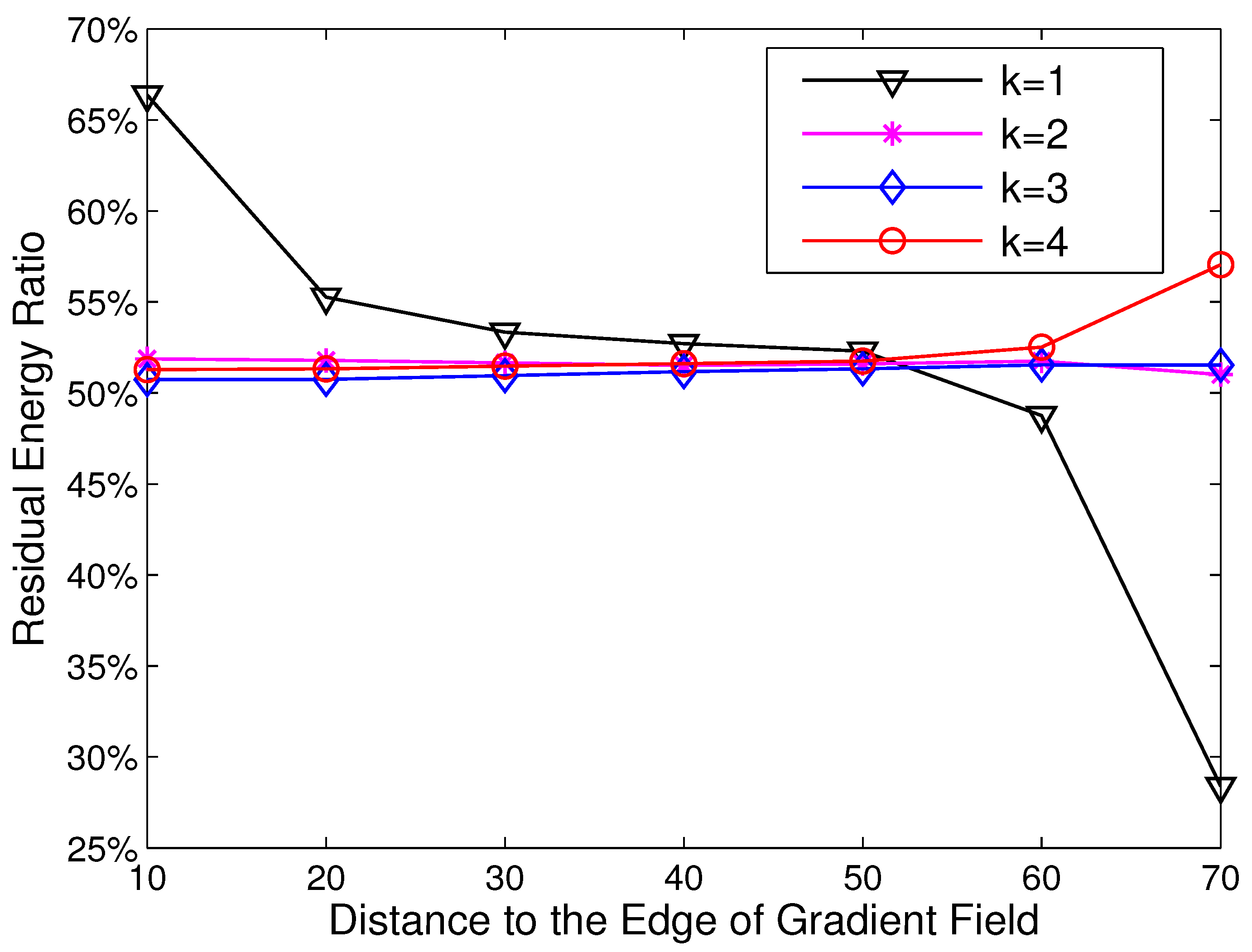
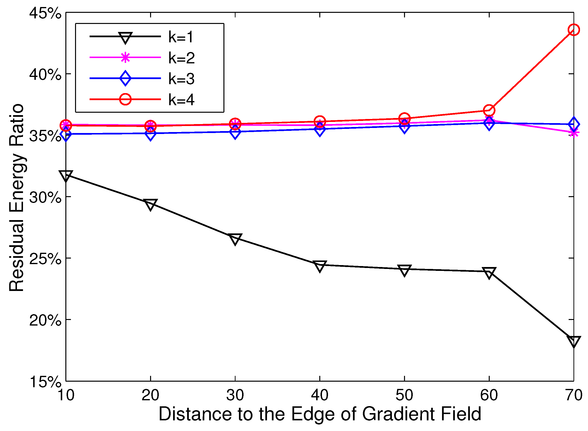
3.3. Imbalanced Energy Consumption in HCR


4. HCR-1 Protocol Description

4.1. Cluster Head Selection in
4.2. Routing Discovery in
4.3. Cluster Formation in
| Algorithm 1 Clustering and routing algorithm in . |
|
4.4. Protocol Properties
5. Simulation Results
| Type | Parameter | Value |
|---|---|---|
| Application | Initial energy | 2 J |
| Data packet size (l) | 125 Bytes | |
| Sink location | ||
| Round | 20 TDMA frames | |
| Radio model | 50 nJ/bit | |
| 10 pJ/bit/m2 | ||
| 5 nJ/bit/signal |
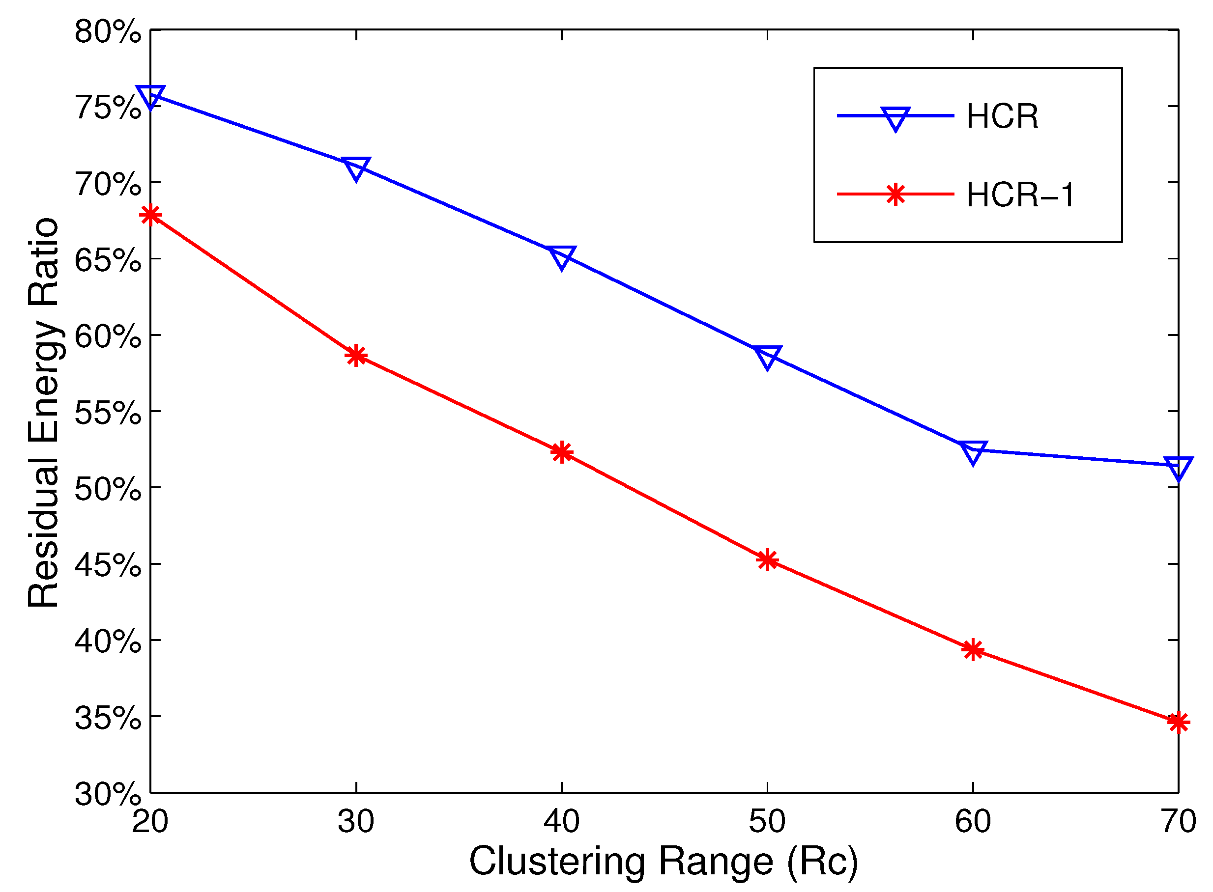
5.1. Parameter Settings

5.2. Energy Consumption Analysis


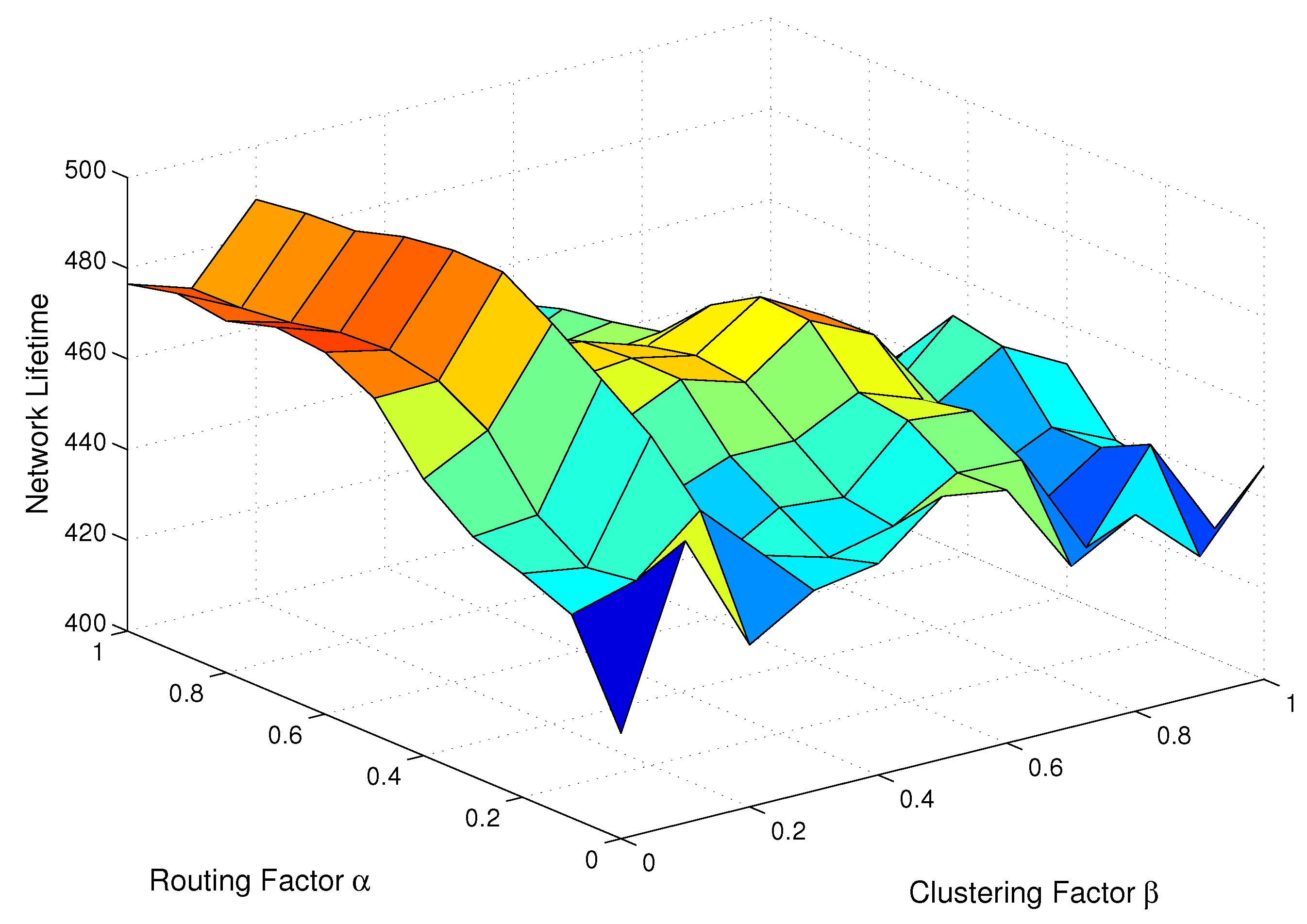
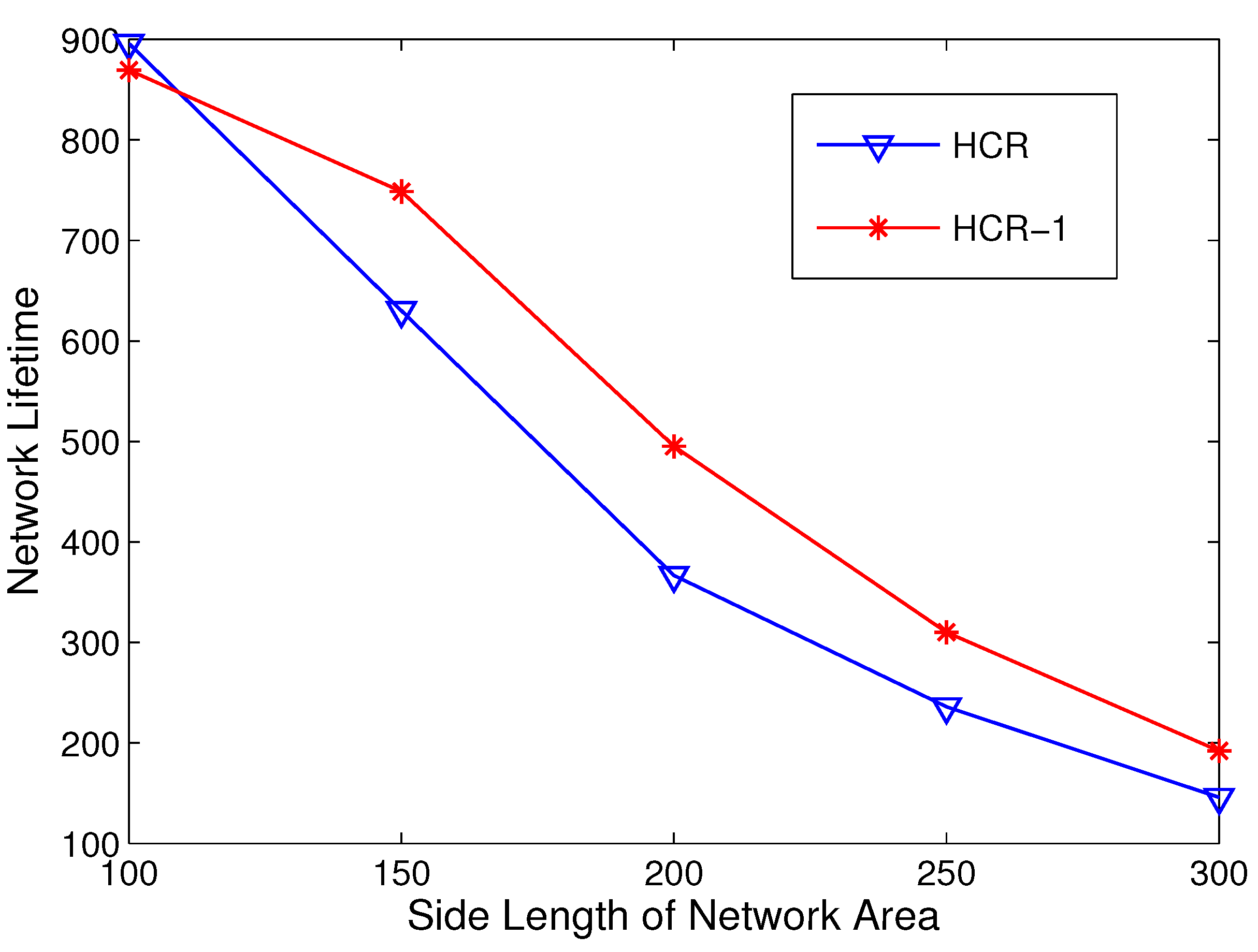
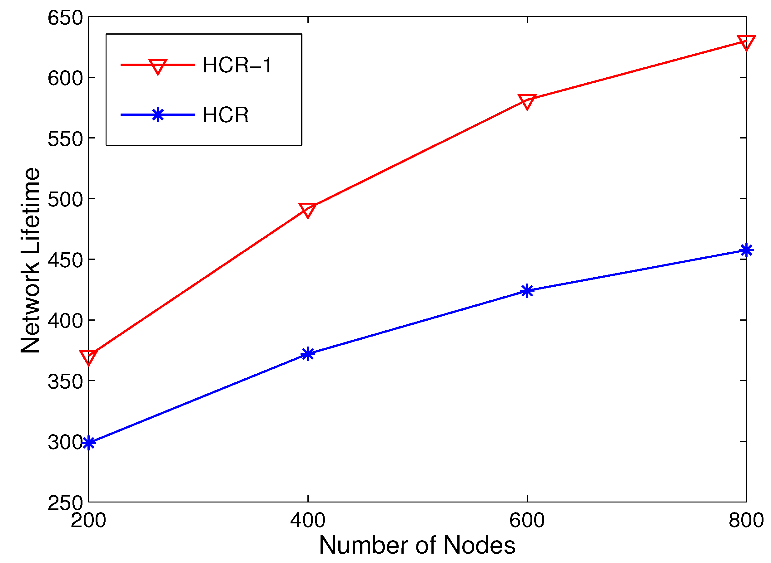
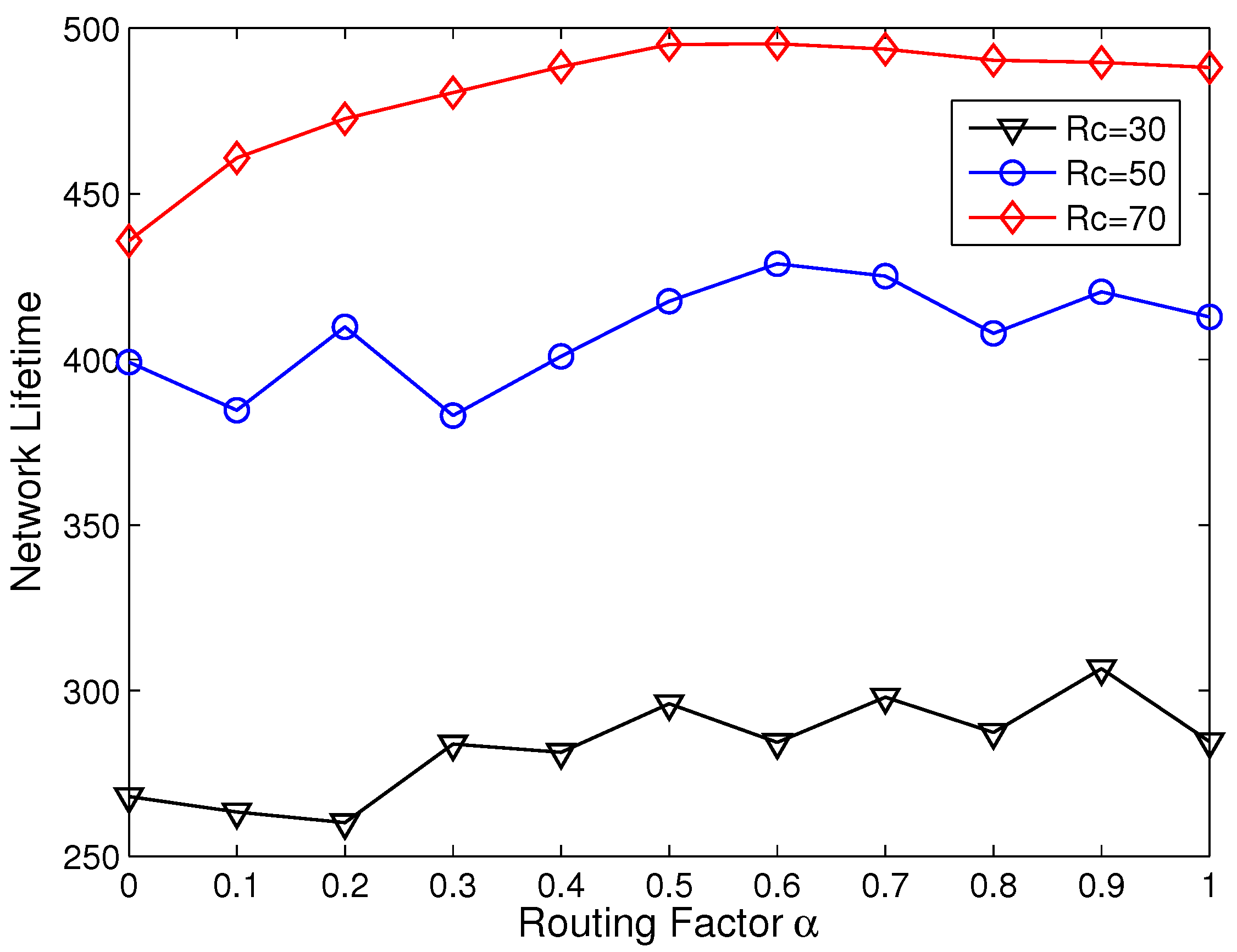
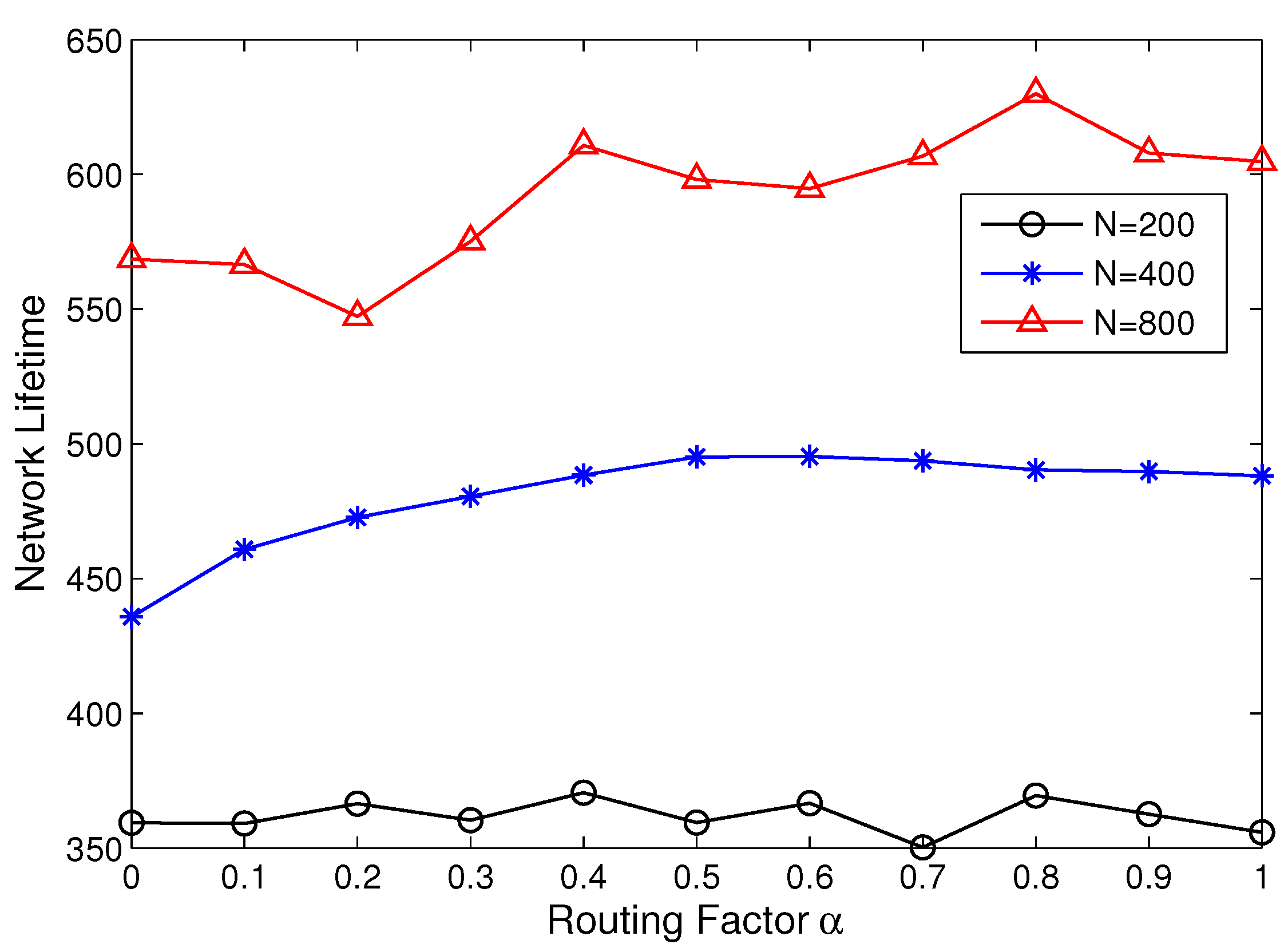
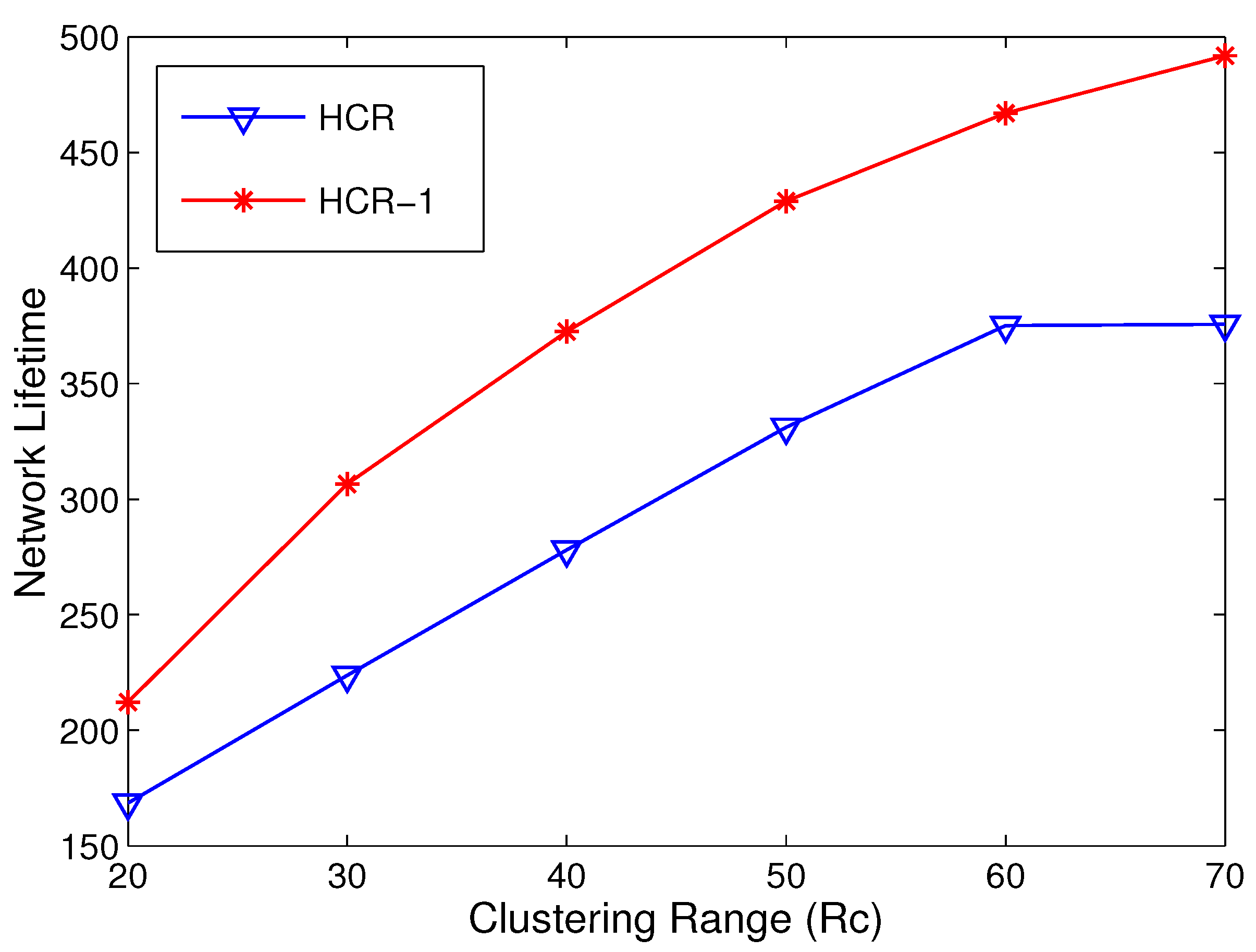
5.3. Network Lifetime Comparison


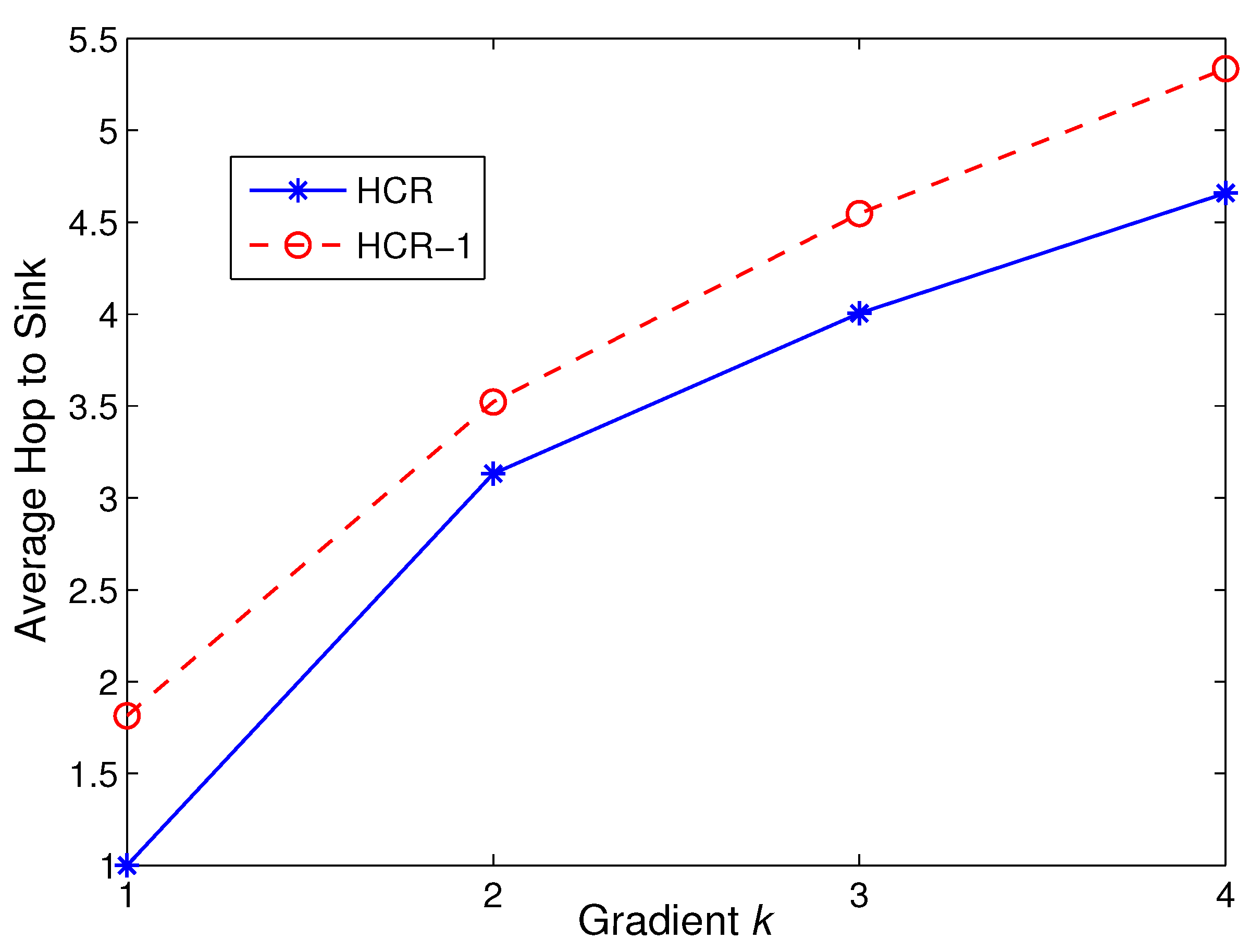
5.4. Transmission Latency Analysis
6. Conclusions
Acknowledgments
Author Contributions
Conflicts of Interest
References
- Akyildiz, I.; Su, W.; Sankarasubramaniam, Y.; Cayirci, E. Wireless sensor networks: A survey. Comput. Netw. 2002, 38, 393–422. [Google Scholar] [CrossRef]
- Gungor, V.C.; Hancke, G.P. Industrial wireless sensor networks: Challenges, design principles, and technical approaches. IEEE Trans. Ind. Electron. 2009, 56, 4258–4265. [Google Scholar] [CrossRef]
- Chen, C.; Yan, J.; Lu, N.; Wang, Y.; Yang, X.; Guan, X. Ubiquitous Monitoring for Industrial Cyber-Physical Systems over Relay Assisted Wireless Sensor Networks. IEEE Trans. Emerg. Top. Comput. 2015, 3, 352–362. [Google Scholar] [CrossRef]
- Werner-Allen, G.; Lorincz, K.; Ruiz, M.; Marcillo, O.; Johnson, J.; Lees, J.; Welsh, M. Deploying a wireless sensor network on an active volcano. IEEE Internet Comput. 2006, 10, 18–25. [Google Scholar] [CrossRef]
- Liu, Y.; He, Y.; Li, M.; Wang, J.; Liu, K.; Mo, L.; Dong, W.; Yang, Z.; Xi, M.; Zhao, J.; et al. Does Wireless Sensor Network Scale? A Measurement Study on GreenOrb. In Proceedings of the 30th IEEE International Conference on Computer Communications (INFOCOM), Shanghai, China, 10–15 April 2011; pp. 873–881.
- Liu, Y.; Xiong, N.; Zhao, Y.; Vasilakos, A.V.; Gao, J.; Jia, Y. Multi-layer clustering routing algorithm for wireless vehicular sensor networks. IET Commun. 2010, 4, 810–816. [Google Scholar] [CrossRef]
- Du, R.; Chen, C.; Yang, B.; Lu, N.; Guan, X.; Shen, X. Effective Urban Traffic Monitoring by Vehicular Sensor Networks. IEEE Trans. Veh. Technol. 2015, 64, 273–286. [Google Scholar] [CrossRef]
- Di Francesco, M.; Das, S.K.; Anastasi, G. Data Collection in Wireless Sensor Networks with Mobile Elements: A Survey. ACM Trans. Sens. Netw. 2011, 8. [Google Scholar] [CrossRef]
- Liu, X.Y.; Zhu, Y.; Kong, L.; Liu, C.; Gu, Y.; Vasilakos, A.; Wu, M.Y. CDC: Compressive Data Collection for Wireless Sensor Networks. IEEE Trans. Parallel Distrib. Syst. 2015, 26, 2188–2197. [Google Scholar] [CrossRef]
- Heinzelman, W.B.; Chandrakasan, A.P.; Balakrishnan, H. An application-specific protocol architecture for wireless microsensor networks. IEEE Trans. Wirel. Commun. 2002, 1, 660–670. [Google Scholar] [CrossRef]
- Abbasi, A.A.; Younis, M. A survey on clustering algorithms for wireless sensor networks. Comput. Commun. 2007, 30, 2826–2841. [Google Scholar] [CrossRef]
- Liu, X. A Survey on Clustering Routing Protocols in Wireless Sensor Networks. Sensors 2012, 12, 11113–11153. [Google Scholar] [CrossRef] [PubMed]
- Ye, M.; Li, C.; Chen, G.; Wu, J. EECS: An energy efficient clustering scheme in wireless sensor networks. In Proceedings of the 24th IEEE International Performance Computing and Communications Conference, Phoenix, Arizona, 7–9 April 2005; pp. 535–540.
- Younis, O.; Fahmy, S. HEED: A hybrid, energy-efficient, distributed clustering approach for ad hoc sensor networks. IEEE Trans. Mob. Comput. 2004, 3, 366–379. [Google Scholar] [CrossRef]
- Cao, Y.; He, C. A distributed clustering algorithm with an adaptive backoff strategy for wireless sensor networks. IEICE Trans. Commun. 2006, E89-B, 609–613. [Google Scholar] [CrossRef]
- Fang, S.; Berber, S.; Swain, A. An Overhead Free Clustering Algorithm for Wireless Sensor Networks. In Proceedings of the 2007 IEEE Global Telecommunications Conference (GLOBECOM), Washington, DC, USA, 26–30 November 2007; pp. 1144–1148.
- Amini, N.; Vahdatpour, A.; Xu, W.; Gerla, M.; Sarrafzadeh, M. Cluster size optimization in sensor networks with decentralized cluster-based protocols. Comput. Commun. 2012, 35, 207–220. [Google Scholar] [CrossRef] [PubMed]
- Wei, D.; Jin, Y.; Vural, S.; Moessner, K.; Tafazolli, R. An Energy-Efficient Clustering Solution for Wireless Sensor Networks. IEEE Trans. Wirel. Commun. 2011, 10, 3973–3983. [Google Scholar] [CrossRef]
- Xu, Z.; Long, C.; Chen, C.; Guan, X. Hybrid Clustering and Routing Strategy with Low Overhead for Wireless Sensor Networks. In Proceedings of the 2010 IEEE International Conference on Communications (ICC), Cape Town, South Africa, 23–27 May 2010; pp. 1–5.
- Wei, G.; Ling, Y.; Guo, B.; Xiao, B.; Vasilakos, A.V. Prediction-based data aggregation in wireless sensor networks: Combining grey model and Kalman Filter. Comput. Commun. 2011, 34, 793–802. [Google Scholar] [CrossRef]
- Xu, X.; Ansari, R.; Khokhar, A.; Vasilakos, A.V. Hierarchical Data Aggregation Using Compressive Sensing (HDACS) in WSNs. ACM Trans. Sens. Netw. 2015, 11, 45:1–45:25. [Google Scholar] [CrossRef]
- Hoang, D.C.; Yadav, P.; Kumar, R.; Panda, S.K. Real-Time Implementation of a Harmony Search Algorithm-Based Clustering Protocol for Energy-Efficient Wireless Sensor Networks. IEEE Trans. Ind. Inform. 2014, 10, 774–783. [Google Scholar] [CrossRef]
- Ye, F.; Zhong, G.; Lu, S.; Zhang, L. GRAdient broadcast: A robust data delivery protocol for large scale sensor networks. Wirel. Netw. 2005, 11, 285–298. [Google Scholar] [CrossRef]
- Huang, P.; Chen, H.; Xing, G.; Tan, Y. SGF: A state-free gradient-based forwarding protocol for wireless sensor networks. ACM Trans. Sensor Netw. 2009, 5, 777–781. [Google Scholar] [CrossRef]
- Wang, A.; Yang, D.; Sun, D. A clustering algorithm based on energy information and cluster heads expectation for wireless sensor networks. Comput. Electr. Eng. 2012, 38, 662–671. [Google Scholar] [CrossRef]
© 2015 by the authors; licensee MDPI, Basel, Switzerland. This article is an open access article distributed under the terms and conditions of the Creative Commons Attribution license (http://creativecommons.org/licenses/by/4.0/).
Share and Cite
Xu, Z.; Chen, L.; Liu, T.; Cao, L.; Chen, C. Balancing Energy Consumption with Hybrid Clustering and Routing Strategy in Wireless Sensor Networks. Sensors 2015, 15, 26583-26605. https://doi.org/10.3390/s151026583
Xu Z, Chen L, Liu T, Cao L, Chen C. Balancing Energy Consumption with Hybrid Clustering and Routing Strategy in Wireless Sensor Networks. Sensors. 2015; 15(10):26583-26605. https://doi.org/10.3390/s151026583
Chicago/Turabian StyleXu, Zhezhuang, Liquan Chen, Ting Liu, Lianyang Cao, and Cailian Chen. 2015. "Balancing Energy Consumption with Hybrid Clustering and Routing Strategy in Wireless Sensor Networks" Sensors 15, no. 10: 26583-26605. https://doi.org/10.3390/s151026583
APA StyleXu, Z., Chen, L., Liu, T., Cao, L., & Chen, C. (2015). Balancing Energy Consumption with Hybrid Clustering and Routing Strategy in Wireless Sensor Networks. Sensors, 15(10), 26583-26605. https://doi.org/10.3390/s151026583