Gliding on the Edge: The Impact of Climate Change on the Habitat Dynamics of Two Sympatric Giant Flying Squirrels, Petaurista elegans and Hylopetes phayrei, in South and Southeast Asia

Abstract

South and Southeast Asia are considered biodiversity hotspots, yet they face escalating threats from deforestation and climate change. This study evaluates the suitable habitat extent of two sympatric flying squirrels, Petaurista elegans and Hylopetes phayrei, using ensemble distribution models based on the climate-only model (COM) and habitat–climate model (HCM) approaches. The results indicated severe habitat loss, with suitable areas comprising only 1.56–1.66% (P. elegans) and 0.22–2.47% (H. phayrei) of their estimated extent of occurrence. Within IUCN-defined ranges, the suitability for P. elegans was 28.25% and 30.04%, while H. phayrei showed 2.86% and 32.39% in terms of the HCM and COM, respectively. The analysis further revealed habitat fragmentation, reduced patch size, and edge complexity, with future scenarios predicting increased isolation. These results highlight the urgent necessity for region-specific conservation strategies focusing on habitat recovery, connectivity, and transboundary cooperation. The recommended actions include genetic studies, corridor analysis, and field validation. This research provides critical baseline data to inform integrated, multi-stakeholder conservation planning across South and Southeast Asia for the long-term persistence of these vulnerable flying squirrel species.

1. Introduction

The South and Southeast Asian region is recognized for its exceptional biodiversity, harboring a vast array of flora and fauna [1]. Notably, it contains approximately 15% of the world’s tropical forest cover and exhibits disproportionately high levels of endemism, both at the taxa and higher taxonomic levels, compared to other biomes [2,3]. This region also encompasses several globally significant biodiversity hotspots. Despite its ecological richness, the region has become a major deforestation hotspot in recent decades, significantly contributing to global tropical forest loss [4,5]. Importantly, this region supports the highest diversity of flying squirrels, making it a critical hotspot for this group of mammalian fauna [6].

A total of 57 flying squirrel species are classified into 15 genera globally, forming a monophyletic lineage within the tribe Pteromyini under the subfamily Sciurinae and family Sciuridae. These species are broadly distributed in Eurasia and North America [7,8]. Among them, the giant flying squirrels represent a distinctive lineage of rodents that, despite their ecological importance, have attracted minimal and inconsistent scientific interest [9]. These mammals are integral to forest ecosystem functioning, contributing essential ecosystem services such as pollination and seed dispersal, and they are recognized as important bioindicators of ecosystem health [9,10]. Adapted for aerial locomotion, they possess a specialized gliding membrane known as the patagium, which extends between their limbs and enables efficient movement through the forest canopy. This gliding ability is an evolutionary adaptation to their arboreal lifestyle, enhancing their capacity to exploit spatially distributed resources and evade predators [11,12]. Furthermore, gliding has likely driven the diversification of multiple vertebrate lineages by enabling access to the upper canopy and facilitating the exploitation of arboreal niches more efficiently [13,14]. Despite their ecological importance, flying squirrel populations have experienced significant declines in recent decades, primarily driven by habitat loss resulting from deforestation, degradation of primary forests, and hunting pressures, especially within the biodiversity-rich landscapes of Southeast Asia [15,16,17,18,19].

Among the flying squirrel species, Petaurista elegans and Hylopetes phayrei are sympatric, sharing overlapping distributions across parts of Southeast Asia [20,21]. Specifically, Petaurista elegans (Spotted Giant Flying Squirrel) is a large-bodied species, distinguished by a robust and elongated form, with a head–body length ranging from 320 to 510 mm and a bushy tail nearly equal in length to its body, contributing to aerial stability. It features a broad patagium extending from the wrists to the ankles, facilitating gliding between trees [22]. Morphologically, it is distinguished by dense reddish-brown dorsal fur, paler ventral surfaces, and large eyes adapted for nocturnal activity [23]. In contrast, Hylopetes phayrei (Indochinese Flying Squirrel) is significantly smaller, with a head–body length of approximately 180–220 mm and a relatively shorter tail. It also possesses a well-developed, albeit narrower, patagium and is characterized by soft greyish-brown dorsal fur and whitish underparts. Its smaller size and lighter build enhance its maneuverability within dense forest canopies, allowing for agile gliding [24]. Furthermore, previous studies have demonstrated that tail length in flying squirrels exhibits positive allometric scaling with body size, potentially enhancing aerodynamic control and maneuverability during gliding [25]. Similarly, the patagial surface area has been shown to scale with body mass in a manner that likely reflects evolutionary selection for improved gliding efficiency across species [26]. The most recent evaluations by the IUCN SSC Small Mammal Specialist Group (SMSG) categorized both species as “Least Concern”, with assessments dating back nearly a decade [20,21]. Given the accelerating pace of environmental change, there is a pressing need to generate updated scientific data on the habitat preferences and climate change responses of these species. Such information is essential for guiding the development of a transboundary conservation strategy that includes both these and other sympatric taxa. Comprehensive ecological assessments will facilitate a re-evaluation of both species’ conservation status by the IUCN SSC Small Mammal Specialist Group (SMSG) and provide a robust foundation for broader conservation-focused research. Furthermore, improving our understanding of the synergistic effects of climate change and land cover transformations will yield critical insights into species-specific vulnerabilities, thereby enabling the design of more targeted and effective conservation interventions.

Henceforth, effective species management at both the habitat and landscape scales necessitate a thorough understanding of species distributions and the identification of ecologically suitable habitats [27]. In this regard, species distribution models (SDMs) have become indispensable tools for predicting species occurrences across geographic regions, thereby providing critical insights for habitat management and conservation planning [28,29,30,31]. Recently, the incorporation of both climatic and habitat-specific variables into SDMs has gained prominence, enhancing the ability to forecast potential range shifts under various climate change scenarios [32,33,34]. A systematic assessment of environmentally suitable areas, consistent with a species’ ecological niche and habitat requirements, is fundamental to ensuring long-term species persistence. Furthermore, understanding the interactions between key environmental variables and dynamic climatic conditions is fundamental to the identification and conservation of suitable habitats. Despite the growing application of ecological modeling, only three habitat suitability studies have been conducted recently within South and Southeast Asia, focusing on five Petaurista species [34,35,36]. This limited scope underscores a significant knowledge gap concerning other sympatric species within the same taxonomic group. Addressing this gap is important, particularly through the adoption of adaptive management strategies that incorporate future uncertainties and enhance species resilience across their IUCN-defined ranges. Accordingly, the present study aimed to utilize two modeling approaches viz. a habitat–climate model (HCM) and a climate-only model (COM) to (i) identify suitable habitats for Petaurista elegans and Hylopetes phayrei within their IUCN-designated ranges under current and future climate scenarios; (ii) determine the key predictors influencing their suitable habitats; and (iii) understand the landscape configuration of both species in present and future climatic conditions.

2. Materials and Methods

2.1. Geographic Distribution and Study Area

The IUCN Red List estimates the extent of occurrence (EOO) for P. elegans at approximately 10,003,504 km² and that for H. phayrei at around 3,221,169 km² (Figure 1). Specifically, P. elegans is a widely distributed Asian species occurring across northern South Asia, southern and central China, and much of Southeast Asia (Figure 1). In South Asia, it has been documented in Nepal, Bhutan, and northeastern India, typically at elevations ranging from 3000 to 4000 m above sea level (asl) [24]. In China, its distribution includes the provinces of Yunnan, Sichuan, Guizhou, Xizang (Tibet), Hubei, Hunan, Gansu, and Shaanxi [37]. Within Southeast Asia, P. elegans is widespread, occurring in Myanmar, Vietnam, Lao PDR, Thailand, Peninsular Malaysia, Sabah, Sarawak, and Indonesia (Sumatra and Java) (Figure 1) [38]. In this region, it inhabits elevations ranging from 200 to 4000 m asl, with observations from Peninsular Malaysia highlighting this elevational variability [39]. In contrast, H. phayrei has a more restricted distribution, occurring in Myanmar, Thailand, Lao PDR, northwestern Vietnam, and China (notably in Guizhou and possibly Fujian provinces). Previous reports also suggest its presence on Hainan Island and in Guangxi and Fujian provinces [37]. However, distribution records from Lao PDR remain uncertain, with the 1999 Status Report for Wildlife of Lao PDR noting a lack of confirmed historical specimens and treating its occurrence as provisional [40]. This species typically occupies lower elevations, ranging from sea level up to 1500 m asl [41]. Given that the IUCN SSC Small Mammal Specialist Group (SMSG) has defined distinct extents for both species, the IUCN-defined extents were adopted as the spatial training domain for developing and evaluating the species distribution models (SDMs) in this study. It provides a standardized and expert-reviewed approximation of the species’ known or inferred distribution. Although the range may not indicate confirmed presence at all locations, it offers a reliable basis for large-scale modeling and conservation assessments. Hence, the IUCN-designated range was used as the study area for both species in the two modeling approaches in present and future climatic scenarios.

2.2. Secondary Occurrence Records

The study utilized primarily presence records obtained from secondary sources. Specifically, occurrence data were retrieved from the GeoCAT platform, which aggregates biodiversity information from multiple reputable databases [42]. A total of 73 occurrence records for P. elegans and 45 for H. phayrei were compiled within their respective IUCN-defined ranges (Figure 1). Moreover, to minimize potential model overfitting and spatial sampling bias, only direct and indirect observations from secondary sources were used, while records from captive individuals or preserved museum specimens were excluded, ensuring that only georeferenced occurrences from natural habitats were included for model calibration. To further control for spatial autocorrelation and sampling redundancy, the occurrence points were spatially rarefied to a minimum distance of 4.5 km utilizing SDM Toolbox v2.4 [43]. This resolution was particularly chosen to match with the spatial grain of the environmental raster layers employed in the modeling process, thereby enhancing model performance and reliability by minimizing spatial autocorrelation effects.

2.3. Covariate Selection

The predictor variables used in the species distribution modeling (SDM) were categorized into four groups: bioclimatic, topographic, habitat, and anthropogenic variables (Table S1) [44]. The 19 bioclimatic variables were obtained from the WorldClim database (https://www.worldclim.org/) [45]. According to the recent IUCN assessments, Petaurista elegans is primarily associated with montane and evergreen forests, whereas Hylopetes phayrei occupies montane and deciduous forests. Accordingly, Euclidean distances to these specific forest types, viz., montane (euc_111), evergreen (euc_112), and deciduous (euc_124), were included as key habitat predictors [20,21,46]. These habitat layers were derived from Copernicus Land Cover data and processed using the Euclidean Distance tool in ArcGIS v10.8 [46]. Moreover, the topographic variables, such as elevation, slope, and aspect, were extracted from the Shuttle Radar Topography Mission (SRTM) digital elevation model at a 90 m spatial resolution (http://srtm.csi.cgiar.org/srtmdata/, accessed on 2 November 2024. The anthropogenic pressures were presented by the Global Human Footprint Dataset, applied as a proxy for the Human Influence Index (HII) (hum_foot), which quantifies cumulative human impacts on natural ecosystems [47]. The environmental predictors were resampled and standardized to a spatial resolution of 30 arcseconds (~4.5 km²) by using the Spatial Analyst extension in ArcGIS v10.6, ensuring consistency with species occurrence data and enabling reliable model performance (Table S1).

Two distinct modeling approaches were implemented in this study: the climate-only model (COM) and habitat–climate model (HCM), each utilizing different sets of predictor variables. The HCM incorporated variables from all four categories (bioclimatic, habitat, anthropogenic, and topographic), whereas the COM was limited to bioclimatic and topographic variables only. To ensure model robustness and minimize multicollinearity, spatial correlation among predictor variables was evaluated using the VisTrails version 2.2.3 [48]. The predictors with high collinearity (Pearson’s correlation coefficient, r > 0.8) were removed from the final models to avoid redundancy and overfitting (Figures S1–S4) [49]. Furthermore, to further reduce overall redundancy among predictor variables, pairwise Spearman’s and Kendall’s correlation coefficients were also calculated, using the same threshold as applied for Pearson’s correlation. Additionally, to assess the potential impacts of climate change on species distributions, future SDMs were developed under two shared socioeconomic pathways: SSP2–4.5 (intermediate-emissions scenario) and SSP5–8.5 (high-emissions scenario), for two future timeframes—mid-century (2041–2060) and late-century (2061–2080). The climate projections were derived from the HadGEM3-GC31-LL global circulation model, part of the Coupled Model Intercomparison Project Phase 6 (CMIP6), which was selected for its proven reliability in simulating climate dynamics across South and Southeast Asia [50,51,52]. The non-climatic predictors in the HCM framework were held constant in the future projections, ensuring that predicted range shifts could be attributed solely to climatic changes and thereby enhancing ecological relevance and interpretability [36,53].

2.4. Model Preparation and Evaluation

The ensemble SDM framework was adopted to generate robust habitat suitability predictions under two distinct modeling strategies. Hence, by integrating multiple algorithms, this approach leverages the complementary strengths of individual models, thereby improving predictive accuracy and minimizing model-specific biases [54]. Such an integrated methodology is particularly effective in capturing the complex and multifactorial relationships between species distributions and environmental variables. Specifically, four well-established algorithms were employed: Maximum Entropy (MaxEnt), Multivariate Adaptive Regression Splines (MARS), Random Forest (RF), and Generalized Linear Models (GLM) [29,55,56]. These models were implemented through the Software for Assisted Habitat Modeling (SAHM) package within the VisTrails platform [57]. For each modeling strategy, viz., the habitat–climate model (HCM) and the climate-only model (COM), the ensemble outputs comprised two primary components: (i) a continuous habitat suitability surface, with values ranging from 0 (unsuitable) to 1 (highly suitable), and (ii) an ensemble agreement map ranging from 0 to 4, representing the number of algorithms that identified a given pixel as suitable habitat. Notably, pixels with an agreement score of 4 indicate full consensus among all algorithms, thereby reflecting areas of highest predicted suitability and model reliability. Furthermore, to enhance the accuracy of the predictions, continuous habitat suitability outputs were converted into binary presence–absence maps using the sensitivity = specificity (SES) threshold criterion. Model performance was primarily evaluated using the Area Under the Curve (AUC) of the Receiver Operating Characteristic (ROC), with AUC values ≥ 0.75 considered indicative of acceptable predictive accuracy [58,59]. In addition to AUC, a suite of complementary evaluation metrics was calculated across both training and cross-validation datasets (n = 10 replicates), including change in AUC (ΔAUC), True Skill Statistic (TSS), Cohen’s Kappa, Proportion Correctly Classified (PCC), sensitivity, and specificity. To assess the influence of individual environmental predictors, their relative contributions were averaged across all four modeling algorithms, offering valuable insights into the key ecological drivers underlying species distributions [60,61,62,63].

2.5. Landscape Configuration Assessment

To enable comparative analyses, the qualitative and geometric attributes of suitable habitat patches for both target species were systematically assessed under current and projected future climatic scenarios across both modeling approaches. This evaluation employed class-level landscape metrics generated using FRAGSTATS version 4.2.1, a widely recognized tool in landscape ecology and environmental planning [64]. FRAGSTATS offers a comprehensive analytical framework for quantifying spatial patterns and configurations of habitat patches, providing critical insights into landscape structure and habitat dynamics [65]. This study utilized a suite of key landscape metrics to assess patch morphology and spatial configuration, including number of patches (NP), patch density (PD), Total Edge (TE), Largest Patch Index (LPI), Landscape Shape Index (LSI), and Aggregation Index (AI). Together, these metrics provide a detailed perspective on habitat fragmentation, spatial continuity, and structural complexity. Specifically, NP and PD quantify the frequency and spatial distribution of habitat patches, while TE and LPI characterize edge complexity and the relative dominance of the largest contiguous habitat patch, respectively. The LSI serves as an indicator of geometric complexity, capturing deviations from simple, compact patch shapes. In contrast, the AI quantifies the degree of spatial cohesion among patches, thereby reflecting the extent of clustering versus dispersion across the landscape. Together, these metrics offer essential ecological context for interpreting habitat suitability under varying climate scenarios. Hence, understanding the landscape configuration is crucial for maintaining viable populations and informing current conservation strategies [66].

3. Results

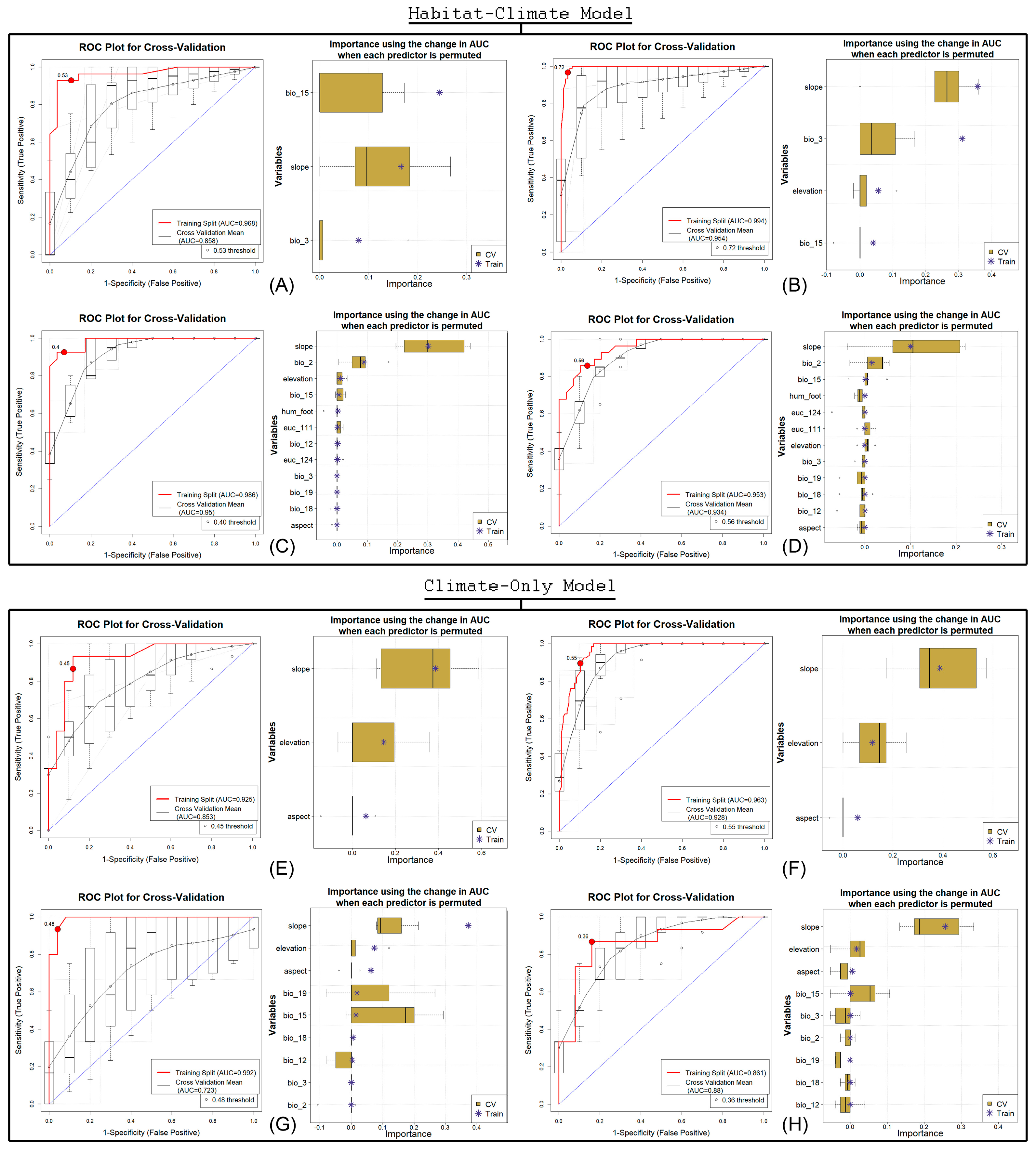
3.1. Model Evaluation and Assessment

Both modeling approaches within the ensemble species distribution framework demonstrated strong predictive performance for both P. elegans and H. phayrei across training and cross-validation datasets (Figure 2 and Figure 3,

Table 1. The table summarizes the model performance metrics for each modeling technique employed under both approaches as well as for the final ensemble model used to estimate habitat suitability for Petaurista elegans and Hylopetes phayrei. A total of five modeling algorithms were applied, each evaluated with an AUC threshold of 0.75. These included Maximum Entropy (MaxEnt), Random Forest (RF), Generalized Linear Models (GLM), and Multivariate Adaptive Regression Splines (MARS). The various key metrics include AUC (Area Under the Curve), ΔAUC (difference between training and cross-validation AUC), PCC (Proportion Correctly Classified), and TSS (True Skill Statistic). HCM: habitat–climate model; COM: climate-only model.

Species	Modeling Approach	Model	Dataset	AUC	ΔAUC	PCC	TSS	Kappa	Specificity	Sensitivity
Petaurista elegans	HCM	GLM	Train	0.968	0.097	91.2	0.825	0.825	0.897	0.929
			CV	0.871		86.4	0.727	0.727	0.867	0.86
		MARS	Train	0.927	0.028	83.5	0.671	0.671	0.837	0.833
			CV	0.899		80.2	0.601	0.602	0.818	0.783
		MaxEnt	Train	0.986	0.052	92.9	0.857	0.857	0.931	0.926
			CV	0.934		79.7	0.587	0.588	0.827	0.76
		RF	Train	0.934	0.006	82.5	0.649	0.649	0.828	0.821
			CV	0.928		83.8	0.68	0.677	0.827	0.853
	COM	GLM	Train	0.968	0.026	91.2	0.825	0.825	0.897	0.929
			CV	0.942		88.2	0.76	0.763	0.9	0.86
		MARS	Train	0.811	0.047	77.6	0.555	0.497	0.781	0.774
			CV	0.764		72.3	0.437	0.387	0.717	0.721
		MaxEnt	Train	0.982	0.041	92.9	0.857	0.857	0.931	0.926
			CV	0.941		82.1	0.633	0.636	0.867	0.767
		RF	Train	0.956	0.012	86	0.719	0.719	0.862	0.857
			CV	0.944		87.8	0.76	0.757	0.827	0.933
Hylopetes phayrei	HCM	GLM	Train	0.968	0.110	91.2	0.825	0.825	0.897	0.929
			CV	0.858		84.7	0.693	0.693	0.833	0.86
		MARS	Train	0.994	0.04	96.7	0.934	0.934	0.968	0.966
			CV	0.954		91.6	0.829	0.83	0.936	0.893
		MaxEnt	Train	0.986	0.036	92.9	0.857	0.857	0.931	0.926
			CV	0.95		87.8	0.76	0.756	0.86	0.9
		RF	Train	0.953	0.019	86	0.719	0.719	0.862	0.857
			CV	0.934		82.5	0.653	0.651	0.793	0.86
	COM	GLM	Train	0.925	0.072	87.5	0.747	0.737	0.88	0.867
			CV	0.853		82.5	0.64	0.646	0.84	0.8
		MARS	Train	0.963	0.035	89.7	0.794	0.785	0.898	0.896
			CV	0.928		84.1	0.671	0.664	0.862	0.81
		MaxEnt	Train	0.992	0.269	94.9	0.892	0.892	0.958	0.933
			CV	0.723		66.4	0.777	0.782	0.896	0.689
		RF	Train	0.861	0.019	85	0.707	688	0.84	0.867
			CV	0.88		85	0.653	0.669	0.92	0.733

). In the HCM approach, the highest training AUC was achieved by the MaxEnt algorithm for P. elegans (AUC = 0.986), while for H. phayrei, the MARS model yielded the highest AUC of 0.994. In the COM approach, the MaxEnt algorithm again produced the highest training AUC values for both species, with 0.982 for P. elegans and 0.992 for H. phayrei. In terms of model performance during cross-validation, the MaxEnt algorithm attained the highest AUC for P. elegans (AUC = 0.934) and H. phayrei (AUC = 0.950) under the HCM approach. Conversely, in the COM approach, the RF model achieved the highest AUC for P. elegans (AUC = 0.944), while the MARS model performed best for H. phayrei (AUC = 0.928). Notably, the greatest ΔAUC was observed in the GLM model under the HCM approach, with values of 0.097 and 0.110 for P. elegans and H. phayrei, respectively, suggesting potential model overfitting. Conversely, the Random Forest (RF) model exhibited the lowest ΔAUC values for both species within the HCM framework, indicating superior generalizability. A comparable trend was observed in the COM framework, where the Generalized Linear Models (GLM) method demonstrated the highest ΔAUC for P. elegans and MaxEnt for H. phayrei, whereas RF consistently maintained the lowest ΔAUC values across both species. Furthermore, additional evaluation metrics, including Pearson’s correlation coefficient (PCC), True Skill Statistic (TSS), Cohen’s Kappa, sensitivity, and specificity, consistently produced high scores across both modeling approaches and species, thereby reinforcing the robustness and predictive reliability of the ensemble models (Figure 2 and Figure 3; Table 1).

3.2. Variable Importance in Two Modeling Approaches

The ensemble models yielded critical insights into the relative contributions of environmental predictors for both species across the two modeling frameworks (Figure 2 and Figure 3;

Table 2. The relative variable importance scores for predictor variables across four modeling algorithms (GLM, MARS, MaxEnt, and Random Forest) for two species (Petaurista elegans and Hylopetes phayrei) and two modeling approaches (COM and HCM). Values represent the scaled variable importance (ranging from 0 to 1) derived from each algorithm. For GLM, importance is based on the absolute standardized coefficients of variables retained in the final model. For MARS, importance reflects the cumulative contribution of each variable to model performance as estimated by the reduction in Generalized Cross-Validation (GCV) error. MaxEnt and Random Forest importance values are based on permutation importance and mean decrease in accuracy, respectively. The average contribution (μ) and relative percentage (%) across all four algorithms are also shown. bio_2: mean diurnal range (mean of monthly (max temp − min temp)); bio_3: isothermality (Bio2/Bio7); bio_12: annual precipitation; bio_15: precipitation seasonality (coefficient of variation); bio_18: precipitation of warmest quarter; bio_19: precipitation of coldest quarter; Euclidean distance to montane forests: euc_111; Euclidean distance to evergreen forests: euc_112; Euclidean distance to deciduous forests: euc_124; Human Influence Index: hum_foot; COM: climate-only model; HCM: habitat–climate model.

Species	Approach	Variables	GLM	MARS	MaxEnt	RF	μ (Mean)	μ (Mean) %
Petaurista elegans	HCM	aspect	0.000	0.000	0.002	0.000	0.001	0.11
		bio_12	0.000	0.000	0.000	0.000	0.000	0.00
		bio_15	0.258	0.040	0.051	0.035	0.096	20.12
		bio_18	0.000	0.000	0.000	0.000	0.000	0.00
		bio_3	0.079	0.310	0.017	0.000	0.102	21.28
		elevation	0.000	0.056	0.009	0.000	0.016	3.42
		euc_111	0.000	0.000	0.000	0.000	0.000	0.00
		euc_112	0.000	0.000	0.080	0.000	0.020	4.19
		hum_foot	0.000	0.000	0.000	0.000	0.000	0.01
		slope	0.148	0.358	0.313	0.151	0.243	50.86
	COM	aspect	0.000	0.000	0.000	0.000	0.000	0.00
		bio_12	0.000	0.000	0.000	0.000	0.000	0.00
		bio_15	0.312	0.040	0.042	0.010	0.101	23.37
		bio_18	0.000	0.000	0.003	0.000	0.001	0.18
		bio_3	0.057	0.310	0.025	0.001	0.098	22.78
		elevation	0.000	0.056	0.017	0.000	0.018	4.23
		slope	0.205	0.358	0.256	0.035	0.213	49.45
Hylopetes phayrei	HCM	aspect	0.000	0.000	0.000	0.000	0.000	0.00
		bio_12	0.228	0.000	0.002	0.000	0.058	9.81
		bio_15	0.139	0.000	0.005	0.003	0.037	6.23
		bio_18	0.180	0.000	0.002	0.000	0.046	7.76
		bio_19	0.000	0.000	0.000	0.000	0.000	0.00
		bio_2	0.000	0.000	0.003	0.000	0.001	0.12
		bio_3	0.365	0.000	0.093	0.000	0.115	19.53
		elevation	0.000	0.165	0.161	0.004	0.082	14.04
		euc_111	0.444	0.267	0.002	0.003	0.179	30.52
		euc_124	0.045	0.000	0.000	0.000	0.011	1.91
		hum_foot	0.000	0.000	0.128	0.000	0.032	5.44
		slope	0.000	0.000	0.000	0.109	0.027	4.63
	COM	aspect	0.063	0.059	0.063	0.006	0.048	9.59
		bio_12	0.000	0.000	0.003	0.000	0.001	0.14
		bio_15	0.000	0.000	0.015	0.001	0.004	0.81
		bio_18	0.000	0.000	0.006	0.000	0.001	0.28
		bio_19	0.000	0.000	0.018	0.000	0.004	0.90
		bio_2	0.000	0.000	0.000	0.000	0.000	0.00
		bio_3	0.000	0.000	0.000	0.000	0.000	0.00
		elevation	0.145	0.118	0.074	0.017	0.088	17.79
		slope	0.386	0.387	0.372	0.257	0.350	70.49

). For P. elegans, within the HCM framework, slope was identified as the predominant predictor, accounting for 50.86% of the model’s explanatory power, followed by bio_3 (isothermality) and bio_15 (precipitation seasonality), which contributed 21.28% and 20.12%, respectively. A similar pattern was observed in the COM approach, where slope again had the highest contribution at 49.45%, followed by bio_15 (23.37%) and bio_3 (22.78%), indicating that topographic and climatic seasonality variables play a dominant role in determining habitat suitability for this species. In contrast, for H. phayrei, the most influential variable in the HCM approach was the Euclidean distance to montane forest (euc_111), contributing 30.52%, highlighting the species’ strong habitat association. This was followed by bio_3 (19.53%) and elevation (14.04%). Interestingly, in the COM approach, slope became the most dominant predictor, contributing a substantial 70.49%, followed by elevation with a contribution of 17.79%. These results underscore the differing ecological drivers for each species and modeling approach, with topography and forest habitat proximity playing pivotal roles in shaping their distribution (Table 2).

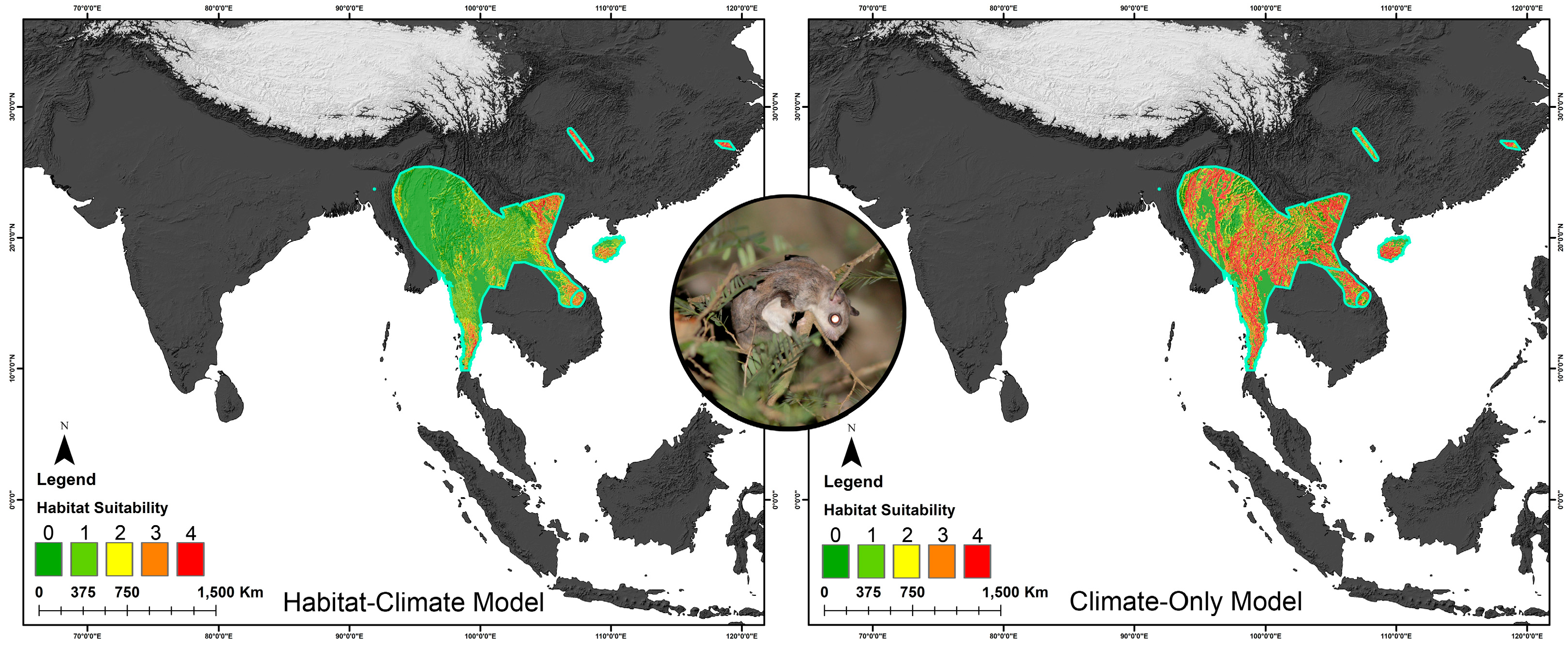
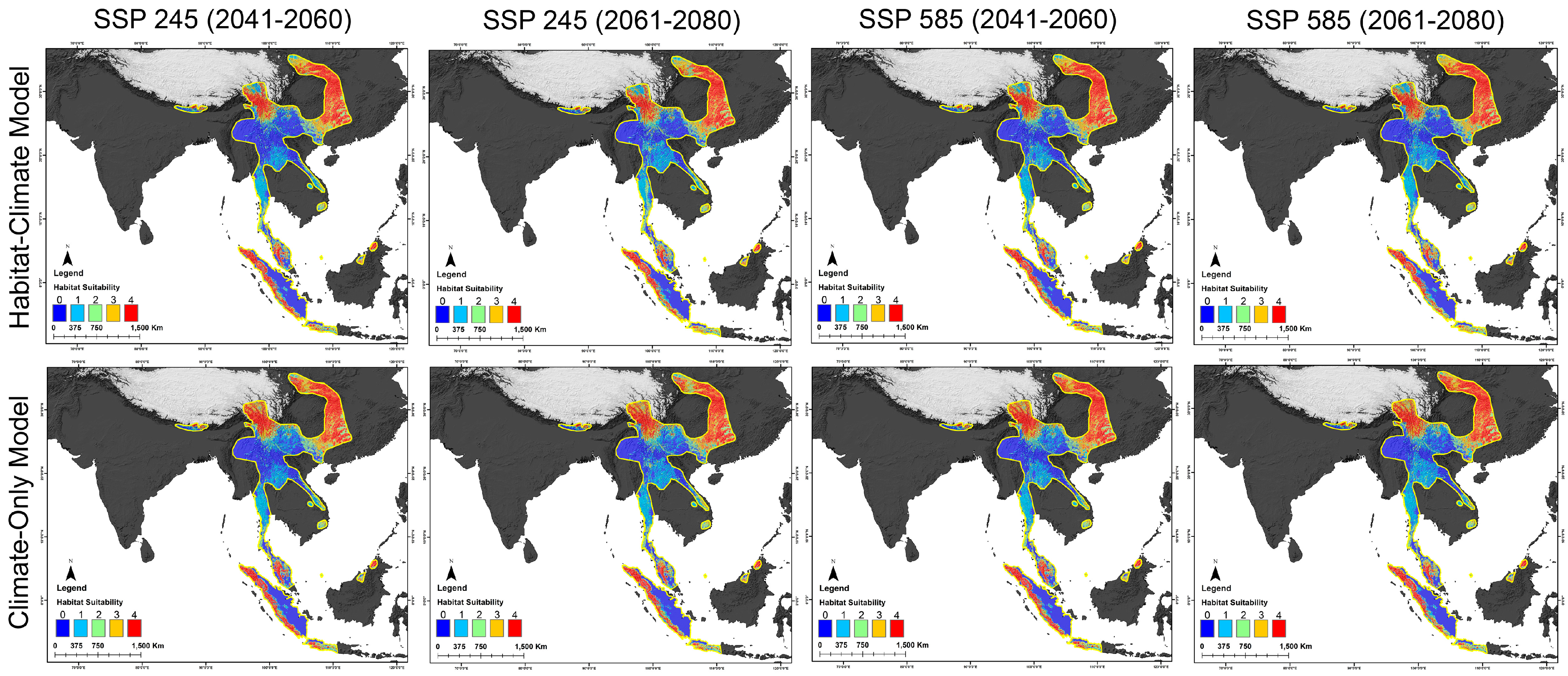
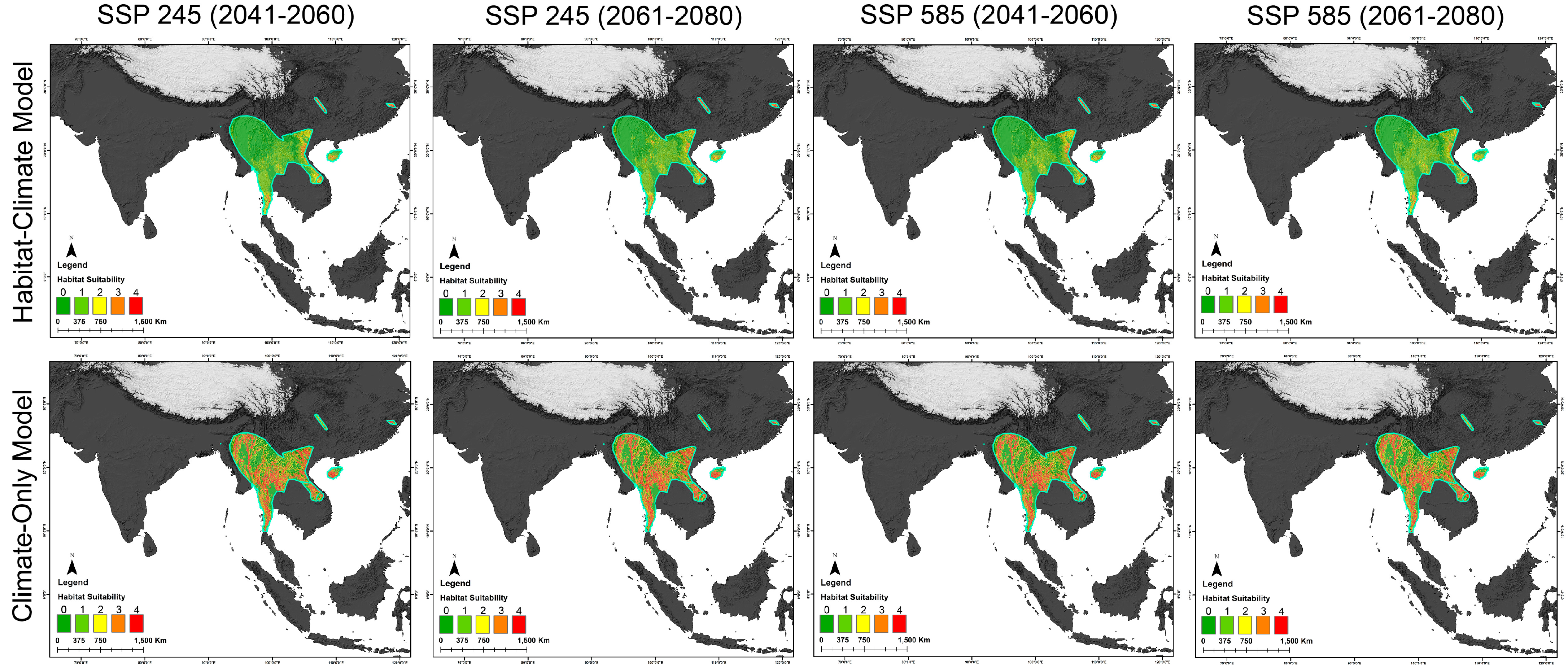
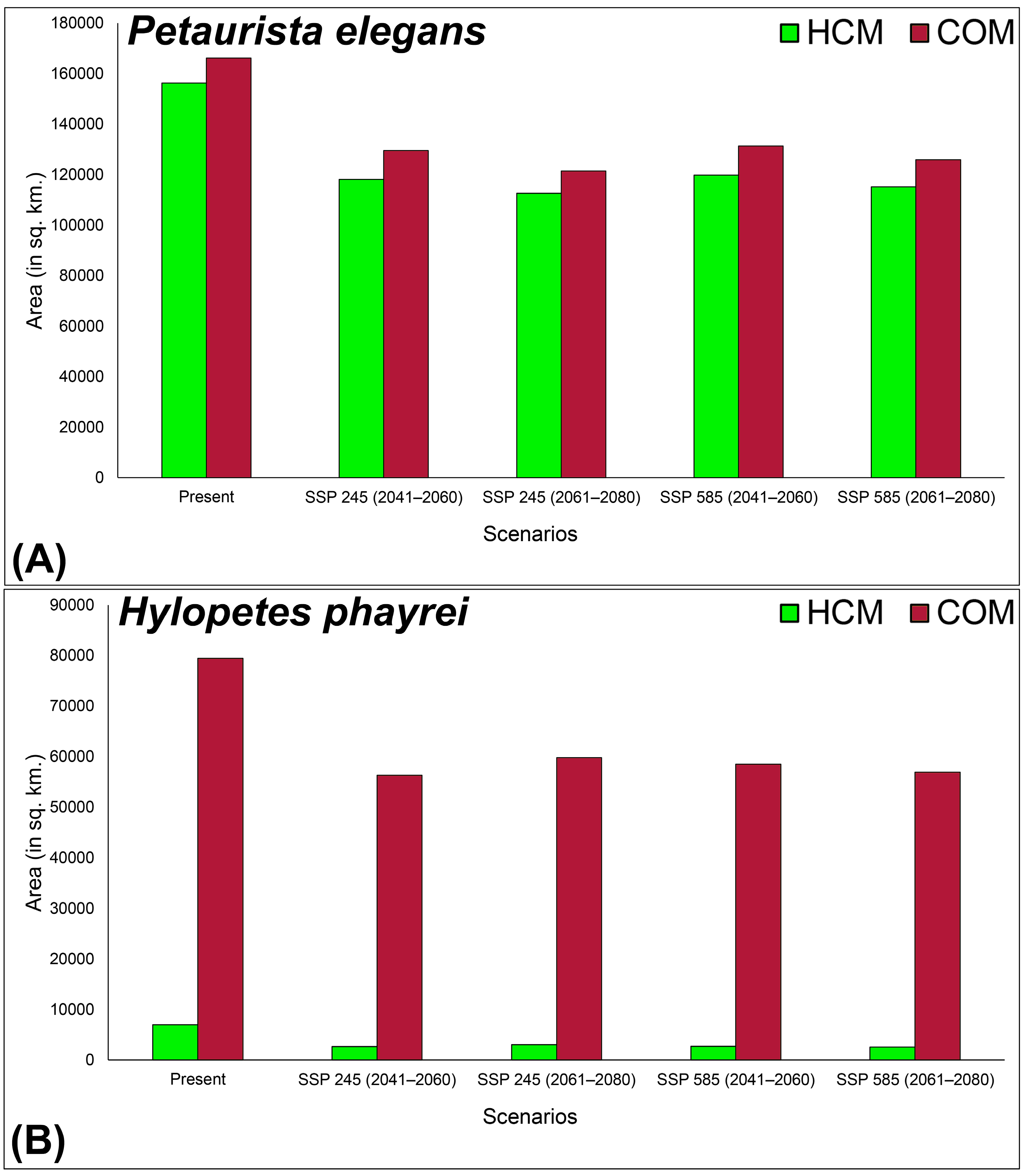
3.3. Habitat Dynamics in Present and Future

The assessment of habitat suitability revealed concerning trends, as the models identified only a small fraction of the estimated EOO as suitable under current climatic conditions (Figure 4 and Figure 5, Table S2). Specifically, for P. elegans, only 1.56% and 1.66% of the total EOO were predicted as suitable habitat under the HCM and COM approaches, respectively. For H. phayrei, the suitable area was even more limited, with only 0.22% (HCM) and 2.47% (COM) of its EOO identified as suitable (Figure 4 and Figure 5). When habitat suitability was evaluated within the IUCN-defined range boundaries in the present scenario, the suitable habitat for P. elegans accounted for just 28.25% (HCM) and 30.04% (COM). In the case of H. phayrei, suitable habitat represented only 2.86% under the HCM approach and 32.39% under the COM approach in the present scenario (Figure 4 and Figure 5, Table S2).

Furthermore, under future climatic scenarios, the projections from both modeling approaches revealed a concerning trend of declining habitat suitability for both species (Figure 6, Figure 7 and Figure 8). Specifically, in the HCM approach for P. elegans, suitable habitat was projected to decline by 26.34% to 26.38% compared to current conditions. For H. phayrei, the decline was more severe, ranging between 56.42% and 62.82% under the same approach. Similarly, the COM approach also indicated a reduction in suitable areas. For P. elegans, habitat suitability was projected to decline by 20.95% to 26.89%, while for H. phayrei, a decline of up to 29.08% is expected under future climate scenarios (Figure 6, Figure 7 and Figure 8, Table S2). These findings emphasize the potential susceptibility of both species to climate change, especially H. phayrei, and underscore the critical necessity for adaptive conservation strategies that integrate projected future climate scenarios.

3.4. Habitat Shape Geometry

The anticipated reduction in suitable habitat area for both species under future climate scenarios is accompanied by significant changes in their spatial configuration (

Table 3. Landscape metrics describing habitat shape geometry of Petaurista elegans and Hylopetes phayrei under present and future scenarios, evaluated using both the habitat–climate model (HCM) and climate-only model (COM) approaches. Metrics include number of patches (NP), patch density (PD), Total Edge (TE), Largest Patch Index (LPI), Landscape Shape Index (LSI), and Aggregation Index (AI).

Species	Approach	Scenario	NP	PD	LPI	TE	LSI	AI
Petaurista elegans	HCM	Present	651	3,001,949	15.2705	1144.5	36.5282	80.8217
		SSP 245 (2041–2060)	399	1,840,174	10.5029	894.936	32.7815	75.2138
		SSP 245 (2061–2080)	449	2,070,772	10.3516	894.684	33.5994	69.2102
		SSP 585 (2041–2060)	403	1,858,622	11.1277	888.384	32.3425	73.6517
		SSP 585 (2061–2080)	397	1,830,950	11.026	871.08	32.4063	67.2352
	COM	Present	599	2,762,162	16.8868	1130.556	34.9584	82.2072
		SSP 245 (2041–2060)	342	1,577,292	10.1311	964.656	33.7765	76.5359
		SSP 245 (2061–2080)	396	1,826,338	9.6707	964.236	34.8906	69.2237
		SSP 585 (2041–2060)	365	1,683,367	10.5038	959.952	33.4152	75.9
		SSP 585 (2061–2080)	358	1,651,083	10.5347	947.184	33.6597	64.3357
Hylopetes phayrei	HCM	Present	106	1,103,088	0.6076	109.956	16.3625	59.652
		SSP 245 (2041–2060)	52	541,226.8	0.1744	44.688	10.8571	52.8166
		SSP 245 (2061–2080)	47	489,185.7	0.1763	48.384	10.8679	50.0458
		SSP 585 (2041–2060)	57	593,267.8	0.1744	46.62	11.1	50.1307
		SSP 585 (2061–2080)	52	541,226.8	0.1744	43.512	10.5714	47.8616
	COM	Present	565	5,879,666	20.637	1020.096	45.6541	66.0939
		SSP 245 (2041–2060)	461	4,797,391	6.6196	803.88	42.7232	62.3236
		SSP 245 (2061–2080)	499	5,192,837	9.3713	839.496	43.2641	60.9305
		SSP 585 (2041–2060)	480	4,995,114	7.0307	826.98	42.9913	59.6983
		SSP 585 (2061–2080)	469	4,880,643	6.7517	813.288	43.0311	55.2882

). Notably, for P. elegans, both modeling approaches indicated a marked decrease in the number of suitable habitat patches. NP decreased markedly by 31.02% to 39.01% in the HCM approach and by 33.88% to 42.90% in the COM approach, indicating the disappearance of several habitat patches in future projections (Table 3). Correspondingly, PD also declined, which reflects a reduction in patch frequency across the landscape. Furthermore, the size of remaining patches declined significantly, as shown by a reduction in the LPI of up to 32.21% in the HCM approach and 42.73% in the COM approach. This downsizing led to decreased TE, while the simplification of patch geometry was evidenced by a lower LSI. These changes collectively point to increased fragmentation, with habitat patches becoming more isolated from one another. This is further supported by a decline in the AI, highlighting reduced spatial cohesion and greater separation between suitable habitat areas under future conditions (Table 3).

A similar pattern of habitat degradation was observed for Hylopetes phayrei under both modeling approaches within its range. Notably, the reduction in suitable patches was even more pronounced for this species. NP declined by up to 55.66% in the HCM approach and 18.40% in the COM approach, indicating a significant loss of habitat patches in future projections. This loss resulted in a marked decrease in patch density, as reflected by the declining PD values. Additionally, the size of the remaining habitat patches decreased considerably, accompanied by a reduction in TE and a simplification of patch shapes, as indicated by declines in the LPI, TE, and ED. These trends suggest that the patches not only became smaller but also more geometrically uniform. The suitable area fragmentation is further underscored by a substantial decline in the AI, which dropped by 19.76% in the HCM approach and 16.34% in the COM approach, signifying increased spatial isolation of remaining suitable areas (Table 3).

Collectively, these findings for both P. elegans and H. phayrei under both modeling frameworks illustrate the severe impacts of climate change. The suitable habitats were not only significantly reduced and, in some cases, completely lost, but the remaining patches tended to be smaller, simpler in shape, and more widely dispersed across the landscape in future scenarios.

4. Discussion

Recognizing that South and Southeast Asian countries are currently facing significant threats to wildlife due to intensifying anthropogenic pressures necessitates implementation of comprehensive conservation and management strategies [5]. It is particularly concerning that the protected areas of this region have experienced some of the highest levels of human-induced disturbances globally over the past decade [67,68]. In response, several initiatives for research and monitoring have been attempted to develop and enforce effective conservation and management strategies specific to the region’s unique ecological and socio-political contexts [69]. These strategies must adopt a multifaceted approach, integrating broader conservation goals with targeted management of protected areas. In light of this urgent need, the present study focuses on two sympatric species of flying squirrels found across South and Southeast Asia. Hence, by analyzing their distribution patterns under current and projected climate and anthropogenic scenarios, this study aims to support the formulation of adaptive, evidence-based management plans. Ultimately, these findings can inform the design of transboundary conservation initiatives, promoting coordinated efforts for biodiversity preservation across national borders in an era of rapid environmental change.

Therefore, before formulating effective conservation and management plans, it is crucial to delineate the extent of climatically suitable habitats and assess their responses to projected climate change to inform climate-resilient strategies. This study addresses this imperative by modeling the potential distributions of P. elegans and H. phayrei across their extensive geographic ranges in South and Southeast Asia. Utilizing two distinct modeling frameworks, HCM and COM, this study provides valuable insights to guide conservation planning under evolving climatic conditions. Despite the wide geographical distribution of both species across multiple countries in the continent, both modeling approaches revealed only a small proportion of their range as climatically suitable [20,21]. Specifically, the predicted suitable habitats represent a considerably smaller extent within both the designated IUCN range and the estimated EOO. This discrepancy highlights the need to reassess the current IUCN distribution maps, which may overestimate the species’ actual range by incorporating areas of potential but unverified presence. These findings underscore the vulnerability of both species and reinforce the urgency of identifying and prioritizing key habitat patches for future conservation interventions. Moreover, the observed variation in predicted suitable area between the two modeling approaches can be attributed to methodological differences. The HCM approach, by integrating bioclimatic, habitat, anthropogenic, and topographic variables, provided a more ecologically comprehensive depiction of the species’ realized niche. In contrast, the COM approach focused primarily on climatic and topographic variables, omitting habitat-specific constraints. Consequently, the COM approach yielded a slightly broader estimate of potential habitat, though it may be less ecologically restrictive. This comparative analysis underscores the value of employing multiple modeling frameworks to capture the full range of ecological and climatic factors influencing species distributions. Nevertheless, these suitable areas identified in this study constitute only a small fraction of the total estimated EOO and the IUCN-defined range, a finding that is particularly concerning in light of the accelerating habitat loss across Southeast Asia [70,71].

In both modeling frameworks, bioclimatic variables emerged as the most influential predictors governing the distribution of both species. Specifically, variables such as bio_3 (isothermality) and bio_15 (precipitation seasonality) consistently contributed significantly to habitat suitability models for P. elegans and H. phayrei. These temperature- and precipitation-related variables have also been recognized as important ecological drivers for other congeners, thus supporting previous findings [34,35,36,72,73,74]. The prominence of these variables highlights the pivotal role of climatic factors in determining habitat suitability and underscores the potential influence of climate change on future species distributions. Within the HCM approach, Euclidean distance to evergreen forest emerged as the primary habitat predictor for P. elegans, while Euclidean distance to montane forest was most influential for H. phayrei, reinforcing their known habitat preferences, as reported in IUCN assessments. Additionally, slope consistently emerged as an important topographic predictor for both species across the two modeling approaches. This finding is consistent with previous research suggesting that slope can influence microhabitat use by affecting canopy structure, tree spacing, and opportunities for launching and landing [75]. Moreover, it highlights the challenges gliding squirrels face in gap-bridging, energetic constraints, and forest structural requirements [76]. Collectively, these findings suggest that the association with sloped terrain may reflect broader habitat characteristics, such as increased canopy connectivity, optimal launch heights, or a denser understory that are closely associated with slope.

Notably, future projections from both modeling approaches reveal alarming trends, suggesting that both species are likely to experience substantial habitat loss and increased fragmentation under climate change scenarios. Interestingly, the HCM approach exhibited a greater degree of habitat decline compared to the COM approach. This discrepancy can be attributed to the more comprehensive nature of the HCM model, which integrates habitat-specific variables alongside climatic factors, offering a more ecologically holistic estimation of suitable areas [77]. These projected habitat losses are consistent with patterns observed in other congeneric species within the region, as well as among various small mammals. This supports prior research demonstrating that species with restricted distributions are particularly vulnerable to climate-driven range contractions, which, in turn, elevate their risk of extinction [78,79,80]. Furthermore, H. phayrei was found to be more susceptible to climate change than P. elegans within their respective IUCN-defined extents. This increased vulnerability may be attributed to the smaller geographic range of H. phayrei, as species with more restricted distributions are generally more susceptible to environmental changes, as shown in previous studies [81,82]. In the case of P. elegans, regions projected to experience the greatest decline in future habitat suitability include northern Myanmar, southern and southeastern China, eastern India, the Malay Peninsula, and Sumatra. These areas should be considered priorities for conservation, as they currently support suitable habitats that are likely to be substantially impacted by climate change. Similarly for H. phayrei, the most severe reductions are anticipated in central Myanmar, Thailand, Laos, and Vietnam under both climate scenarios. These regions currently represent core areas of high habitat suitability, indicating that climate-driven changes may have particularly detrimental effects on the species’ persistence across this landscape. The degradation of viable habitat has not only resulted in the complete loss of some suitable patches but also in significant reductions in the size and spatial extent of those remaining. This has led to a marked decrease in patch area (as indicated by the LPI) and edge complexity (as shown by TE), reinforcing the conclusion that climate change is driving habitat fragmentation. Furthermore, the decline in the Aggregation Index (AI) under future climate scenarios signifies increased spatial isolation of habitat patches, undermining landscape connectivity. This is concerning, as previous research has demonstrated that habitat fragmentation presents significant challenges to flying squirrels by creating gaps that impede their gliding locomotion, thereby disrupting key behaviors such as foraging, mating, and dispersal [83]. In light of these findings, it is crucial to develop region-specific conservation strategies focused on preserving critical habitats and maintaining connectivity. Thus, facilitating safe gap crossings is essential for sustaining metapopulation connectivity, and conserving habitats is necessary to mitigate species decline [36,84,85]. Collectively, it is important to understand the importance of landscape configuration in maintaining viable populations and to inform current conservation strategies [66].

Given the concerning scenario projected under future climate conditions, it is strongly recommended that the IUCN SSC Small Mammal Specialist Group (SMSG), along with regional researchers, initiate systematic, field-based surveys across the broader landscape to verify the actual distribution of the species beyond currently delineated ranges. The habitat patches identified as suitable under both present and future scenarios should be prioritized for ground-truthing to confirm species presence and assess habitat quality and viability. Furthermore, conservation planners and managers in the region must act with urgency to halt ongoing habitat degradation. Statutory governmental agencies should implement and enforce stricter land-use policies to curb the conversion of forested habitats into anthropogenic landscapes. Additionally, particular emphasis must be placed on fostering collaborative transboundary conservation initiatives among mainland range countries, including India, Nepal, Bangladesh, Myanmar, China, Thailand, and Malaysia. Likewise, targeted measures are needed in the island ecosystems of Malaysia and Indonesia, where geographic isolation amplifies the species’ extinction risk. In areas identified as suitable habitats, community-based awareness programs along forest fringes are essential to mitigate anthropogenic threats, such as hunting and the illegal wildlife trade, both of which remain prevalent in Southeast Asia and pose significant risks to small mammal populations. Moreover, delineating connectivity among suitable habitat patches both within and beyond the IUCN-defined distributional ranges is essential. This necessitates the formulation of an integrated management strategy aimed at preserving and sustaining these ecological corridors to facilitate gap-bridging and ensure long-term species conservation. In addition, population-level genetic studies are crucial to elucidate the species’ population structure, genetic diversity, and phylogenetic relationships. Such data would provide a vital baseline for evidence-based conservation planning and can also inform strategies for other lesser-known small mammal species in the region. Ultimately, the integration of local communities, statutory bodies, conservation managers, transboundary cooperative networks, and non-governmental organizations is crucial to assure the long-term conservation of both P. elegans and H. phayrei, along with their associated small mammal fauna, throughout their natural range.

5. Conclusions

The South and Southeast Asian region encompasses several globally recognized biodiversity hotspots, supporting a rich diversity of endemic and threatened species, yet it remains under constant threat from both climatic changes and escalating anthropogenic pressures. In this study, two ensemble SDM approaches, viz., HCM and COM, were employed to identify and prioritize suitable habitats for two sympatric and lesser-known flying squirrel species, P. elegans and H. phayrei. Both species exhibit overlapping distributions across this biogeographically complex region. The study aimed to assess the current extent of suitable habitat for these species and to project future changes under anticipated climate change scenarios. The key aspects evaluated included habitat suitability, patch quality, spatial configuration, and potential habitat connectivity. The results revealed a concerning trend of habitat decline for both species under future climate scenarios, with climate change emerging as the primary driver of range contraction. The critical bioclimatic variables, particularly temperature and precipitation metrics, were found to significantly influence habitat suitability, underscoring the strong dependence of the species on forest ecosystems. In light of these findings, the study proposes several conservation actions, such as population genetic assessments to investigate gene flow and genetic structure, corridor connectivity analyses to address habitat fragmentation, and targeted field surveys for ground-truthing model outputs and validating current species distributions. In addition, the study highlights the urgent need for integrative conservation strategies that involve collaboration among local communities, statutory agencies, transboundary conservation authorities, scientific experts, and non-governmental organizations. Overall, this research provides essential baseline information to guide future conservation planning and field assessments across transboundary landscapes in South and Southeast Asia. Hence, a critical foundation is established for the development of regionally coordinated management strategies aimed at safeguarding these understudied yet ecologically important flying squirrel species.

References

1. Stibig, H.-J.; Achard, F.; Carboni, S.; Raši, R.; Miettinen, J. Change in Tropical Forest Cover of Southeast Asia from 1990 to 2010. Biogeosciences 2014, 11, 247–258. [Google Scholar] [CrossRef]
2. Sodhi, N.S.; Posa, M.R.C.; Lee, T.M.; Bickford, D.; Koh, L.P.; Brook, B.W. The State and Conservation of Southeast Asian Biodiversity. Biodivers. Conserv. 2010, 19, 317–328. [Google Scholar] [CrossRef]
3. Hughes, A.C. Understanding the Drivers of Southeast Asian Biodiversity Loss. Ecosphere 2017, 8, e01624. [Google Scholar] [CrossRef]
4. Hansen, M.C.; Potapov, P.V.; Moore, R.; Hancher, M.; Turubanova, S.A.; Tyukavina, A.; Thau, D.; Stehman, S.V.; Goetz, S.J.; Loveland, T.R.; et al. High-Resolution Global Maps of 21st-Century Forest Cover Change. Science 2013, 342, 850–853. [Google Scholar] [CrossRef]
5. Estoque, R.C.; Ooba, M.; Avitabile, V.; Hijioka, Y.; DasGupta, R.; Togawa, T.; Murayama, Y. The Future of Southeast Asia’s Forests. Nat. Commun. 2019, 10, 1829. [Google Scholar] [CrossRef]
6. Koli, V.K. Biology and conservation status of flying squirrels (Pteromyini, Sciuridae, Rodentia) in India: An update and review. Proc. Zool. Soc. 2016, 69, 9–21. [Google Scholar] [CrossRef]
7. Casanovas-Vilar, I.; Garcia-Porta, J.; Fortuny, J.; Sanisidro, Ó.; Prieto, J.; Querejeta, M.; Llácer, S.; Robles, J.M.; Bernardini, F.; Alba, D.M. Oldest skeleton of a fossil flying squirrel casts new light on the phylogeny of the group. eLife 2018, 7, e39270. [Google Scholar] [CrossRef] [PubMed]
8. Burgin, C.J.; Colella, J.P.; Kahn, P.L.; Upham, N.S. How many species of mammals are there? J. Mammal. 2018, 99, 615. [Google Scholar] [CrossRef]
9. Carey, A.B.; Harrington, C.A. Small mammals in young forests: Implications for management for sustainability. For. Ecol. Manag. 2001, 154, 289–309. [Google Scholar] [CrossRef]
10. Nandini, R.; Parthasarathy, N. Food habits of the Indian giant flying squirrel (Petaurista philippensis) in a rain forest fragment, Western Ghats. J. Mammal. 2008, 89, 1550–1556. [Google Scholar] [CrossRef]
11. Dudley, R.; Byrnes, G.; Yanoviak, S.P.; Borrell, B.; Brown, R.M.; McGuire, J.A. Gliding and the functional origins of flight: Biomechanical novelty or necessity? Annu. Rev. Ecol. Evol. Syst. 2007, 38, 179–201. [Google Scholar] [CrossRef]
12. Chaitanya, R.; McGuire, J.A.; Karanth, P.; Meiri, S. Their fates intertwined: Diversification patterns of the Asian gliding vertebrates may have been forged by dipterocarp trees. Proc. R. Soc. B 2023, 290, 20231379. [Google Scholar] [CrossRef] [PubMed]
13. Byrnes, G.; Spence, A.J. Ecological and biomechanical insights into the evolution of gliding in mammals. Integr. Comp. Biol. 2011, 51, 991–1001. [Google Scholar] [CrossRef]
14. McGuire, J.A.; Dudley, R. The biology of gliding in flying lizards (genus Draco) and their fossil and extant analogs. Integr. Comp. Biol. 2011, 51, 983–990. [Google Scholar] [CrossRef]
15. Lin, Y.S.; Progulske, D.R.; Lee, P.F.; Day, Y.T. Bibliography of Petauristinae (Rodentia, Sciuridae). J. Taiwan Mus. 1985, 38, 49–57. [Google Scholar]
16. Lee, P.F.; Liao, C.Y. Species Richness and Research Trend of Flying Squirrels. J. Taiwan Mus. 1998, 51, 1–20. [Google Scholar]
17. Umapathy, G.; Kumar, A. The Occurrence of Arboreal Mammals in the Rain Forest Fragments in Anamalai Hills, South India. Biol. Conserv. 2000, 92, 311–319. [Google Scholar] [CrossRef]
18. Kumara, H.N.; Singh, M. Distribution and Relative Abundance of Giant Squirrels and Flying Squirrels in Karnataka, India. Mammalia 2006, 70, 40–47. [Google Scholar] [CrossRef]
19. Puyravaud, J.P.; Davidar, P.; Laurance, W.F. Cryptic Destruction of India’s Native Forests. Conserv. Lett. 2010, 3, 390–394. [Google Scholar] [CrossRef]
20. Molur, S. Petaurista elegans. The IUCN Red List of Threatened Species. 2016, e.T16719A22272724. Available online: https://www.iucnredlist.org/species/16719/22272724 (accessed on 17 February 2025). [CrossRef]
21. Tizard, R.J. Hylopetes phayrei. The IUCN Red List of Threatened Species. 2016, e.T10605A22244042. Available online: https://www.iucnredlist.org/species/10605/22244042 (accessed on 17 February 2025). [CrossRef]
22. Byrnes, G.; Lim, N.T.; Spence, A.J. Take-Off and Landing Kinetics of a Free-Ranging Gliding Mammal, the Malayan Colugo (Galeopterus variegatus). Proc. Biol. Sci. 2008, 275, 1007–1013. [Google Scholar] [CrossRef]
23. Thorington, R.W., Jr.; Hoffmann, R.S. Family Sciuridae. In Mammal Species of the World; Wilson, D.E., Reader, D.M., Eds.; The John Hopkins University Press: Baltimore, MD, USA, 2005; pp. 754–818. [Google Scholar]
24. Molur, S.; Srinivasulu, C.; Srinivasulu, B.; Walker, S.; Nameer, P.O.; Ravikumar, L. Status of Non-Volant Small Mammals: Conservation Assessment and Management Plan (C.A.M.P) Workshop Report; Zoo Outreach Organisation/CBSG-South Asia: Coimbatore, India, 2005. [Google Scholar]
25. Stafford, B.J.; Thorington, R.W.; Kawamichi, T. Gliding Behavior of Japanese Giant Flying Squirrels (Petaurista leucogenys). J. Mammal. 2002, 83, 553–562. [Google Scholar] [CrossRef]
26. Jackson, S.M. Glide Angle in the Genus Petaurus and a Review of Gliding in Mammals. Mammal Rev. 2000, 30, 9–30. [Google Scholar] [CrossRef]
27. Ortega-Huerta, M.A.; Peterson, A.T. Modelling spatial patterns of biodiversity for conservation prioritization in North-Eastern Mexico. Divers. Distrib. 2004, 10, 39–54. [Google Scholar] [CrossRef]
28. Guisan, A.; Zimmermann, N.E. Predictive habitat distribution models in ecology. Ecol. Model. 2000, 135, 147–186. [Google Scholar] [CrossRef]
29. Elith, J.; Leathwick, J.R. Species distribution models: Ecological explanation and prediction across space and time. Annu. Rev. Ecol. Evol. Syst. 2009, 40, 677–697. [Google Scholar] [CrossRef]
30. Pearson, R.G. Species’ distribution modeling for conservation educators and practitioners. Netw. Conserv. Educ. Pract. Cent. Biodivers. Conserv. Am. Mus. Nat. Hist. 2010, 3, 54–89. [Google Scholar] [CrossRef]
31. Kujala, H.; Moilanen, A.; Araújo, M.B.; Cabeza, M. Conservation planning with uncertain climate change projections. PLoS ONE 2013, 8, e53315. [Google Scholar] [CrossRef]
32. Eyre, A.C.; Briscoe, N.J.; Harley, D.K.P.; Lumsden, L.F.; McComb, L.B.; Lentini, P.E. Using species distribution models and decision tools to direct surveys and identify potential translocation sites for a critically endangered species. Divers. Distrib. 2022, 28, 700–711. [Google Scholar] [CrossRef]
33. Hu, W.; Onditi, K.O.; Jiang, X.; Wu, H.; Chen, Z. Modeling the potential distribution of two species of shrews (Chodsigoa hypsibia and Anourosorex squamipes) under climate change in China. Diversity 2022, 14, 87. [Google Scholar] [CrossRef]
34. Koli, V.K.; Jangid, A.K.; Singh, C.P. Habitat suitability mapping of the Indian giant flying squirrel (Petaurista philippensis Elliot, 1839) in India with ensemble modeling. Acta Ecol. Sin. 2023, 43, 644–652. [Google Scholar] [CrossRef]
35. Abedin, I.; Kamalakannan, M.; Mukherjee, T.; Choudhury, A.; Singha, H.; Abedin, J.; Banerjee, D.; Kim, H.-W.; Kundu, S. Fading into obscurity: Impact of climate change on suitable habitats for two lesser-known giant flying squirrels (Sciuridae: Petaurista) in Northeastern India. Biology 2025, 14, 242. [Google Scholar] [CrossRef] [PubMed]
36. Abedin, I.; Kamalakannan, M.; Mukherjee, T.; Singha, H.; Banerjee, D.; Kim, H.-W.; Kundu, S. Eco-spatial modeling of two giant flying squirrels (Sciuridae: Petaurista): Navigating climate resilience and conservation roadmap in the Eastern Himalaya and Indo-Burma biodiversity hotspots. Life 2025, 15, 589. [Google Scholar] [CrossRef]
37. Smith, A.T.; Xie, Y. A Guide to the Mammals of China; Princeton University Press: Princeton, NJ, USA, 2008. [Google Scholar]
38. Evans, T.D.; Duckworth, J.W.; Timmins, R.J. Field Observations of Larger Mammals in Laos, 1994–1995. Mammalia 2000, 64, 55–100. [Google Scholar] [CrossRef]
39. Thorington, R.W., Jr.; Koprowski, J.L.; Steele, M.A.; Whatton, J.F. Squirrels of the World; The Johns Hopkins University Press: Baltimore, MD, USA, 2012. [Google Scholar]
40. Duckworth, J.W.; Salter, R.E.; Khounboline, K. Wildlife in Lao PDR: 1999 Status Report; IUCN: Vientiane, Laos, 1999. [Google Scholar]
41. Duckworth, W. Hylopetes phayrei (Blyth, 1859). Available online: http://www.ieaitaly.org/samd (accessed on 17 February 2025).
42. Bachman, S.; Moat, J.; Hill, A.W.; de la Torre, J.; Scott, B. Supporting Red List threat assessments with GeoCAT: Geospatial conservation assessment tool. ZooKeys 2011, 150, 117–126. [Google Scholar] [CrossRef] [PubMed]
43. Brown, J.L.; Bennett, J.R.; French, C.M. SDMtoolbox 2.0: The next generation Python-based GIS toolkit for landscape genetic, biogeographic, and species distribution model analyses. PeerJ 2017, 5, e4095. [Google Scholar] [CrossRef]
44. Peterson, A.T.; Soberón, J. Species distribution modeling and ecological niche modeling: Getting the concepts right. Braz. J. Nat. Conserv. 2012, 10, 102–107. [Google Scholar] [CrossRef]
45. Fick, S.E.; Hijmans, R.J. WorldClim 2: New 1-km Spatial Resolution Climate Surfaces for Global Land Areas. Int. J. Climatol. 2017, 37, 4302–4315. [Google Scholar] [CrossRef]
46. Karra, K.; Kontgis, C.; Statman-Weil, Z.; Mazzariello, J.C.; Mathis, M.; Brumby, S.P. Global Land Use/Land Cover with Sentinel-2 and Deep Learning. In Proceedings of the IGARSS 2021—2021 IEEE International Geoscience and Remote Sensing Symposium, Brussels, Belgium, 11–16 July 2021; IEEE: New York, NY, USA, 2021. [Google Scholar]
47. SEDAC. Last of the Wild Project, Version 2, 2005 (LWP-2): Global Human Footprint Dataset (Geographic). Available online: https://gis.earthdata.nasa.gov/portal/home/item.html?id=e1f0028da5d84d0da724b6dc783f3f23 (accessed on 13 November 2024).
48. Morisette, J.T.; Jarnevich, C.S.; Holcombe, T.R.; Talbert, C.B.; Ignizio, D.; Talbert, M.K.; Silva, C.; Koop, D.; Swanson, A.; Young, N.E. VisTrails SAHM: Visualization and workflow management for species habitat modeling. Ecography 2013, 36, 129–135. [Google Scholar] [CrossRef]
49. Warren, D.L.; Glor, R.E.; Turelli, M. ENMTools: A toolbox for comparative studies of environmental niche models. Ecography 2010, 33, 607–611. [Google Scholar] [CrossRef]
50. Andrews, M.B.; Ridley, J.K.; Wood, R.A.; Andrews, T.; Blockley, E.W.; Booth, B.; Burke, E.; Dittus, A.J.; Florek, P.; Gray, L.J.; et al. Historical simulations with HadGEM3-GC3.1 for CMIP6. J. Adv. Model. Earth Syst. 2020, 12, e2019MS001995. [Google Scholar] [CrossRef]
51. Li, L.; Xie, F.; Yuan, N. On the long-term memory characteristic in land surface air temperatures: How well do CMIP6 models perform? Atmos. Ocean. Sci. Lett. 2023, 16, 100291. [Google Scholar] [CrossRef]
52. Gautam, S.; Shany, V.J. Navigating climate change in southern India: A study on dynamic dry-wet patterns and urgent policy interventions. Geosyst. Geoenviron. 2024, 3, 100263. [Google Scholar] [CrossRef]
53. Allen, B.J.; Hill, D.J.; Burke, A.M.; Clark, M.; Marchant, R.; Stringer, L.C.; Williams, D.R.; Lyon, C. Projected future climatic forcing on the global distribution of vegetation types. Philos. Trans. R. Soc. B Biol. Sci. 2024, 379, 20230011. [Google Scholar] [CrossRef]
54. Hao, T.; Elith, J.; Lahoz-Monfort, J.J.; Guillera-Arroita, G. Testing whether ensemble modelling is advantageous for maximising predictive performance of species distribution models. Ecography 2020, 43, 549–558. [Google Scholar] [CrossRef]
55. Guisan, A.; Zimmermann, N.E.; Elith, J.; Graham, C.H.; Phillips, S.; Peterson, A.T. What matters for predicting the occurrences of trees: Techniques, data, or species’ characteristics? Ecol. Monogr. 2007, 77, 615–630. [Google Scholar] [CrossRef]
56. Miller, J. Species distribution modeling. Geogr. Compass 2010, 4, 490–509. [Google Scholar] [CrossRef]
57. Talbert, C.B.; Talbert, M.K. User Manual for SAHM Package for VisTrails. 2012. Available online: https://pubs.usgs.gov/publication/70118102 (accessed on 13 November 2024).
58. Hayes, M.A.; Cryan, P.M.; Wunder, M.B. Seasonally-dynamic presence-only species distribution models for a cryptic migratory bat impacted by wind energy development. PLoS ONE 2015, 10, e0132599. [Google Scholar] [CrossRef] [PubMed]
59. Lavazza, L.; Morasca, S.; Rotoloni, G. On the reliability of the area under the ROC curve in empirical software engineering. In Proceedings of the 27th International Conference on Evaluation and Assessment in Software Engineering, Oulu, Finland, 14–16 June 2023; pp. 93–100. [Google Scholar]
60. Allouche, O.; Tsoar, A.; Kadmon, R. Assessing the accuracy of species distribution models: Prevalence, kappa and the true skill statistic (TSS). J. Appl. Ecol. 2006, 43, 1223–1232. [Google Scholar] [CrossRef]
61. Cohen, J. Weighted kappa: Nominal scale agreement provision for scaled disagreement or partial credit. Psychol. Bull. 1968, 70, 213–220. [Google Scholar] [CrossRef]
62. Jiménez-Valverde, A.; Acevedo, P.; Barbosa, A.M.; Lobo, J.M.; Real, R. Discrimination capacity in species distribution models depends on the representativeness of the environmental domain. Glob. Ecol. Biogeogr. 2013, 22, 508–516. [Google Scholar] [CrossRef]
63. Phillips, S.J.; Elith, J. POC plots: Calibrating species distribution models with presence-only data. Ecology 2010, 91, 2476–2484. [Google Scholar] [CrossRef] [PubMed]
64. McGarigal, K.; Marks, B.J. FRAGSTATS: Spatial Pattern Analysis Program for Quantifying Landscape Structure; Gen. Tech. Rep. PNW-GTR-351; U.S. Department of Agriculture, Forest Service, Pacific Northwest Research Station: Portland, OR, USA, 1995; pp. 122–351. [Google Scholar]
65. Hesselbarth, M.H.K.; Sciaini, M.; With, K.A.; Wiegand, K.; Nowosad, J. landscapemetrics: An open-source R tool to calculate landscape metrics. Ecography 2019, 42, 1648–1657. [Google Scholar] [CrossRef]
66. Levins, R. Extinctions. In Some Mathematical Questions in Biology; Lectures on Mathematics in the Life Sciences; American Mathematical Society: Providence, RI, USA, 1970; Volume 2, pp. 77–107. [Google Scholar]
67. Geldmann, J.; Manica, A.; Burgess, N.D.; Coad, L.; Balmford, A. A Global-Level Assessment of the Effectiveness of Protected Areas at Resisting Anthropogenic Pressures. Proc. Natl. Acad. Sci. USA 2019, 116, 23209–23215. [Google Scholar] [CrossRef]
68. Graham, V.; Geldmann, J.; Adams, V.M.; Negret, P.J.; Sinovas, P.; Chang, H.-C. Southeast Asian Protected Areas Are Effective in Conserving Forest Cover and Forest Carbon Stocks Compared to Unprotected Areas. Sci. Rep. 2021, 11, 23760. [Google Scholar] [CrossRef]
69. Thao, N.P.; Eales, J.; Lam, D.M.; Hien, V.T.; Garside, R. What Are the Impacts of Activities Undertaken in UNESCO Biosphere Reserves on Socio-Economic Wellbeing in Southeast Asia? A Systematic Review. Environ. Evid. 2023, 12, 30. [Google Scholar] [CrossRef] [PubMed]
70. Sodhi, N.S.; Koh, L.P.; Brook, B.W.; Ng, P.K.L. Southeast Asian biodiversity: An impending disaster. Trends Ecol. Evol. 2004, 19, 654–660. [Google Scholar] [CrossRef]
71. Sodhi, N.S. Tropical biodiversity loss and people—A brief review. Basic Appl. Ecol. 2008, 9, 93–99. [Google Scholar] [CrossRef]
72. Okinen, M.; Hanski, I.; Numminen, E.; Valkama, J.; Selonen, V. Promoting species protection with predictive modelling: Effects of habitat, predators, and climate on the occurrence of the Siberian flying squirrel. Biol. Conserv. 2019, 230, 37–46. [Google Scholar] [CrossRef]
73. Selonen, V.; Hongisto, K.; Hänninen, M.; Turkia, T.; Korpimäki, E. Weather and biotic interactions as determinants of seasonal shifts in abundance measured through nest-box occupancy in the Siberian flying squirrel. Sci. Rep. 2020, 10, 14465. [Google Scholar] [CrossRef]
74. Bedoya-Canas, L.E.; López-Hernández, F.; Cortés, A.J. Climate change responses of high-elevation Polylepis forests. Forests 2024, 15, 811. [Google Scholar] [CrossRef]
75. Vernes, K. Gliding Performance of the Northern Flying Squirrel (Glaucomys sabrinus) in Mature Mixed Forest of Eastern Canada. J. Mammal. 2001, 82, 1026–1033. [Google Scholar] [CrossRef]
76. Flaherty, E.A.; Ben-David, M.; Smith, W.P. Quadrupedal Locomotor Performance in Two Species of Arboreal Squirrels: Predicting Energy Savings of Gliding. J. Comp. Physiol. B 2010, 180, 1067–1078. [Google Scholar] [CrossRef] [PubMed]
77. Wan, G.Z.; Li, Q.Q.; Jin, L.; Chen, J. Integrated Approach to Predicting Habitat Suitability and Evaluating Quality Variations of Notopterygium franchetii under Climate Change. Sci. Rep. 2024, 14, 26927. [Google Scholar] [CrossRef] [PubMed]
78. Payne, B.L.; Bro-Jørgensen, J. Disproportionate climate-induced range loss forecast for the most threatened African antelopes. Curr. Biol. 2016, 26, 1200–1205. [Google Scholar] [CrossRef]
79. Dubos, N.; Montfort, F.; Grinand, C.; Nourtier, M.; Deso, G.; Probst, J.M.; Razafimanahaka, J.H.; Andriantsimanarilafy, R.R.; Rakotondrasoa, E.F.; Razafindraibe, P.; et al. Are narrow-ranging species doomed to extinction? Projected dramatic decline in future climate suitability of two highly threatened species. Perspect. Ecol. Conserv. 2022, 20, 18–28. [Google Scholar] [CrossRef]
80. Costa-Pinto, A.L.; Bovendorp, R.S.; Heming, N.M.; Malhado, A.C.; Ladle, R.J. Where could they go? Potential distribution of small mammals in the Caatinga under climate change scenarios. J. Arid Environ. 2024, 221, 105133. [Google Scholar] [CrossRef]
81. Williams, S.E.; Bolitho, E.E.; Fox, S. Climate Change in Australian Tropical Rainforests: An Impending Environmental Catastrophe. Proc. R. Soc. Lond. B Biol. Sci. 2003, 270, 1887–1892. [Google Scholar] [CrossRef]
82. Radchuk, V.; Kramer-Schadt, S.; Fickel, J.; Wilting, A. Distributions of Mammals in Southeast Asia: The Role of the Legacy of Climate and Species Body Mass. J. Biogeogr. 2019, 46, 2350–2362. [Google Scholar] [CrossRef]
83. Howard, J.M. Gap Crossing in Flying Squirrels: Mitigating Movement Barriers through Landscape Management and Structural Implementation. Forests 2022, 13, 2027. [Google Scholar] [CrossRef]
84. Lindenmayer, D. Small patches make critical contributions to biodiversity conservation. Proc. Natl. Acad. Sci. USA 2019, 116, 717–719. [Google Scholar] [CrossRef]
85. Wintle, B.A.; Kujala, H.; Whitehead, A.; Cameron, A.; Veloz, S.; Kukkala, A.; Moilanen, A.; Gordon, A.; Lentini, P.E.; Cadenhead, N.C.R.; et al. Global synthesis of conservation studies reveals the importance of small habitat patches for biodiversity. Proc. Natl. Acad. Sci. USA 2019, 116, 909–914. [Google Scholar] [CrossRef] [PubMed]
Figure 1. Geographic distribution of Petaurista elegans and Hylopetes phayrei across South and Southeast Asia. The map illustrates secondary occurrence points alongside the IUCN-assessed range extents for each species.
Diversity 17 00403 g001
Figure 2. Model evaluation plot showing the average training ROC for both training and cross-validation (CV) and the predictors chosen by the model for the replicate runs under four models in the habitat–climate model and climate-only model for P. elegans. (A,E) Generalized Linear Models (GLM), (B,F) Multivariate Adaptive Regression Splines (MARS), (C,G) Maximum Entropy (MaxEnt), and (D,H) Random Forest (RF).
Diversity 17 00403 g002
Figure 3. Model evaluation plot showing the average training ROC for both training and cross-validation (CV) and the predictors chosen by the model for the replicate runs under four models in the habitat–climate model and climate-only model for H. phayrei. (A,E) Generalized Linear Models (GLM), (B,F) Multivariate Adaptive Regression Splines (MARS), (C,G) Maximum Entropy (MaxEnt), and (D,H) Random Forest (RF).
Diversity 17 00403 g003
Figure 4. Maps depicting suitable habitats for P. elegans identified by the model under the present climatic scenario in the study area using two modeling approaches. The different colors and numbers represent the level of model agreement, with “0” indicating no model agreement and “4” signifying high suitability where all four models concurred. The photograph of the species was taken from the free repository of Wikimedia Commons under the Creative Commons Attribution 4.0.
Diversity 17 00403 g004
Figure 5. Maps depicting suitable habitats for H. phayrei identified by the model under the present climatic scenario in the study area using two modeling approaches. The different colors and numbers represent the level of model agreement, with “0” indicating no model agreement and “4” signifying high suitability where all four models concurred. The photograph of the species was taken from the free repository of Wikimedia Commons under the Creative Commons Attribution 4.0.
Diversity 17 00403 g005
Figure 6. Maps depicting suitable habitats for P. elegans identified by the model under SSP245 and SSP585 future climatic scenarios using the two modeling approaches. The different colors and numbers represent the level of model agreement, with “0” indicating no model agreement and “4” signifying high suitability where all four models concurred.
Diversity 17 00403 g006
Figure 7. Maps depicting suitable habitats for H. phayrei identified by the model under SSP245 and SSP585 future climatic scenarios using the two modeling approaches. The different colors and numbers represent the level of model agreement, with “0” indicating no model agreement and “4” signifying high suitability where all four models concurred.
Diversity 17 00403 g007
Figure 8. Suitable habitat extent (in km2) for two species under current and future climate scenarios based on two modeling approaches. (A) P. elegans and (B) H. phayrei.
Diversity 17 00403 g008