Impact to Coral Reef Populations at Hā‘ena and Pila‘a, Kaua‘i, Following a Record 2018 Freshwater Flood Event

Abstract

Many corals and reef-dwelling organisms are susceptible to the impacts of storm events, which are typically characterized by large inputs of freshwater, sediment, and nutrients. The majority of storm effects are focused on shallow, nearshore reef flats, as low salinity and sedimentation tend to dissipate with depth and distance from shore. In April 2018, record rainfall on the northern coast of Kaua‘i caused extensive flooding and landslides, introducing large amounts of freshwater and sediment into nearshore reefs. Using benthic and fish transects from 2016–2019 and temperature, sediment, and rainfall data gathered pre- and post-flood, this study aimed to quantify and explicate the effects of flooding on the various biotic populations of two reef habitats at Pila‘a and Hā‘ena, Kaua‘i. Results from the shallow Pila‘a reef suggest sediment and freshwater-associated declines in mean urchin abundance (−52.0%) and increases in mean coral bleaching (+54.5%) at the flood-prone eastern sector. Additionally, decreases in mean urchin (−65.7%) and fish (−42.3%) populations were observed at shallow Hā‘ena transects, but not deep sites, supporting the occurrence of depth-specific affliction. Multivariate community-level analyses affirmed much of these results, showing a significant shift in community structure before and after the flood at both Pila‘a and Hā‘ena. The outcomes of this study are pertinent to strategic design and solution development by local aquatic resource managers, especially as anthropogenic climate change continues to increase the frequency, duration, and intensity of storm events.

1. Introduction

Over the past several decades, many coral reef communities have been declining due to local and global anthropogenic stressors [1,2]. Climate change has led to increases in the frequency and intensity of weather events in many regions [3,4,5], including the Hawaiian Islands [6,7]. Generally, storm events can cause substantial damage to reef habitats [8] and, when exacerbated by other factors such as ocean acidification [9,10,11] and warming [12,13,14], may be even more harmful, as previously degraded corals can be more susceptible to future stress [15,16]. Many major weather events oftentimes lead to acute low salinity and subsequent “reef kills”, which can result in high morality of many benthic organisms, such as corals and reef-dwelling invertebrates (e.g., holothuroids, sponges, and crustaceans) [16,17,18,19]. Indeed, a 15–20% reduction in salinity over a 24 h period can produce a lethal osmotic environment for corals and their endosymbionts [20], along with subsequent reduced coral recruitment and increased densities of suspension feeders [21]. Associated sedimentation can also suppress coral metabolism and induce energetically costly immune responses [22]. Thus, post-flooding reductions in salinity, paired with sediment-induced light impairment and suffocation, can cause substantial bleaching and even mortality, particularly on shallow reef flats [16,23]. Moreover, freshwater flooding can bring an influx of nutrients that can catalyze planktonic proliferations, which can further reduce light to corals, influencing growth, bleaching, and mortality [24,25,26,27,28]. Freshwater, sediment, and nutrient inputs generally attenuate as distance from shore increases due to wind, waves, and tidal currents, thus concentrating the heaviest impacts of flooding on shallow nearshore areas [19,29,30].

The effects of storm-related stressors extend to other nearshore taxa as well. Sea urchins (Class: Echinoidea), which play a critical role in maintaining coral reef conditions, are susceptible to changes in salinity. Acute salinity shifts, such as a freshwater discharge or flood event, can result in up to 100% mortality in adult urchins [31]. This can be disruptive to entire ecosystems, as urchins are important in the suppression and modification of macroalgal abundance, distribution, and assemblage [32,33,34,35,36]. Macroalgae generally compete with corals for space, nutrients, and light access, thus lack of algal population regulation can contribute to shifts from coral-dominant to algal-dominant regimes [37,38,39]. These shifts can lead to relatively depauperate communities, which are less resilient and oftentimes have much of their ecological, economic, and social value inhibited.

Although storm events seldom lead to direct fish mortality [40], they have been shown to cause ephemeral and prolonged decreases in the populations of many reef fish taxa [41,42,43]. Potential sources of fish preclusion from storm-impacted areas include high risk from turbid, low light zones [44], intolerance to low salinities [45], or direct physical forcing of fish away from shallow areas by storm action [46]. Larval recruitment dynamics have also been shown to be disturbed by storm events, suggesting juvenile replenishment may occur at lower rates [47,48]. Furthermore, reef fish distribution and composition is controlled by shelter and food availability [49], suggesting that habitat degradation may be an indirect effect driving reef fish exclusion from storm-affected areas. Regardless of the ultimate source of fish decline, major storm events have the capacity to (at least) transiently impact a reef’s fish assemblages, which can have consequences to local fishery productivity and subsistence.

Coral reefs and their associated fauna are highly vulnerable to storm events that reduce salinity in shallow waters [17,18,19]. Flash floods, which are common in Hawai‘i, are typically intense and short in duration. Three major stochastic freshwater flood events and their impacts to coral reefs have previously been documented in Kāne‘ohe Bay, O‘ahu, in 1965 [17], 1988 [19], and 2014 [16]. More recently, during 13–16 April 2018, heavy flooding and landslides occurred on the northern coast of Kaua‘i. According to the National Weather Service, the rain gauge near Hanalei Bay recorded over 1.3 m of rain during 15–16 April 2018, setting the record for the highest rainfall in a 24 h period in the Hawaiian Islands [50]. Flooding events such as these likely affect Hawaiian corals and other reef organisms, although there currently exist few quantitative data to affirm this. This study aimed to measure and evaluate the effects of this flooding event on fish, coral, and urchin populations by drawing from benthic and environmental monitoring data of two reef sites, Hā‘ena and Pila‘a, which are located 22.2 km apart on the north shore of Kaua‘i (Figure 1). Sediment characteristics and rainfall estimates were used to describe and quantify flooding inputs, which were subsequently utilized to make inferences about changes to water salinity and sedimentation post-flood. These environmental data were then related to any community structure and discrete population variations before and after the major storm event. We anticipated overall declines in biota at Hā‘ena’s shallow reef sites, which were separated by depth into deep (>7 m) and shallow (≤7 m) transects. At the ubiquitously shallow (1–2 m) Pila‘a site, we also expected greater impacts to the exposed eastern sector, which is more susceptible to flooding than the western sector due to local circulation patterns and stream inputs [51].

2. Materials & Methods

2.1. Site Descriptions

2.1.1. Pila‘a Reef

Pila‘a surveys were initially instigated in 2016 to assess system recovery from a late 2001 sedimentation event on the East Pila‘a reef sector, which was subsequently surveyed in the summer of 2002. This event was caused by mudslides that were a result of extensive grading [51]. The environmental and biological data from Pila‘a used in this study drew from yearly sampling efforts spanning from 2016 to 2019 [52,53,54,55]. Annual sample sizes of biological and environmental variable surveys at Pila‘a and the second site, Hā‘ena, are presented in

Table 1. Annual sample size of transect surveys (fish, urchin, and coral data) and environmental data (temperature and sediment loads) from 2016–2019. Depth corresponds to shallow (≤7 m) or deep (>7 m) transects at Hā‘ena, whereas sector refers to the East or West portion of the Pila‘a reef.

				Year (n)
Site	Sector/Depth	Variables	Data Collection Method	2016	2017	2018	2019
Hā‘ena	Shallow (≤7 m)	Fish abundance and biomass	Transect surveys	42	112	73	58
		Sea urchins	Transect surveys	42	57	73	58
		Coral bleaching	Transect surveys and CoralNet	42	57	73	58
		Sediments	Bulk grab sample	9	N/D	19	N/D
	Deep (>7 m)	Fish abundance and biomass	Transect surveys	56	99	37	40
		Sea urchins	Transect surveys	56	51	37	40
		Coral bleaching	Transect surveys and CoralNet	56	51	37	40
Pila‘a	East (1–2 m)	Sea urchins	Transect surveys	37	48	39	23
		Coral bleaching and Sarcothelia abundance	Transect surveys and CoralNet	37	48	39	23
		Temperature	Loggers	5	1	4	N/D
		Sediments	Bulk grab sample	7	N/D	5	N/D
	West (1–2 m)	Sea urchins	Transect surveys	13	34	21	27
		Coral bleaching and Sarcothelia abundance	Transect surveys and CoralNet	13	34	21	27
		Temperature	Loggers	3	1	2	N/D
		Sediments	Bulk grab sample	3	N/D	3	N/D

.

Pila‘a is a shallow reef (1–2 m in depth) with a major channel bisecting the reef flat, which has a depth ranging from 9–15 m (m) at the reef’s outer edge. Several shallower channels (1–2 m depth) help to increase circulation. The general circulation patterns show incoming water flowing over the reef flat and exiting through the main channel (Figure 2). Flushing rates and residence times are dependent on high spring tides coinciding with high offshore wave energy, although only moderate flushing is generated by large offshore waves due to a well-developed reef crest [51].

Pila‘a reef has a history of sedimentation caused by extensive grading on the western slope of the Pila‘a stream valley beginning in the mid-1990s. Generally, the eastern sector of the reef is more heavily impacted by freshwater, sediment, and nutrient exposure from flood events than the adjacent western sector due to stream proximity and structure of local circulation patterns (Figure 1 and Figure 2) [51]. This presented the opportunity to assess the effects of the 2018 storm on communities in the high and low potential exposure areas (East and West sectors, respectively). Because the reef flat depth does not exceed 3 m, the possibility of ubiquitous exposure to a post-flood freshwater lens is also likely (consistent with similar outcomes in [16,19]).

The abundance and distribution of Sarcothelia edmondsoni, a blue zooxanthellate octocoral [56], were also examined at Pila‘a, as blooms of this species have been detected around the Main Hawaiian Islands and are potentially indicative of freshwater input and other anthropogenic pollutants [57,58]. Octocorals, which are soft, nonreef building corals (Subclass: Octocorallia, see Supplementary Materials Figure S1), have been used as bioindicators of poor coastal water quality caused by human influence and freshwater input in many countries [59,60,61]. High abundances of the endemic S. edmondsoni have been found at sites influenced by submarine groundwater discharge and seepage around the Main Hawaiian Islands, suggesting the resilience of S. edmondsoni to salinity fluctuation and anthropogenic input [56,58,62].

2.1.2. Hā‘ena Reef

Field surveys at Hā‘ena also occurred from 2016 to 2019 and were initiated to establish baselines and determine the efficacy of management actions imposed on fishing [50,57,63,64]. The Hā‘ena reserve is divided into management zones of differing fishing pressure. Sampling occurred within and outside this fishing reserve (Figure 1); however, fishing pressure was not found to have a confounding influence on changes to fish populations from 2017 to 2018 [50]. At both Hā‘ena and Pila‘a, surveys were restricted to summer months in order to avoid any confounding effects of seasonal change.

The exposed north shore of Kaua‘i is characterized by high wave energy with the North Pacific Swell as the main forcing function and dominant driver of benthic communities. Two perennial streams intersect the Hā‘ena ahupua‘a (land division) originating in the valleys of Mānoa and Limahuli. They provide a significant freshwater contribution to the nearshore biotic composition.

Unlike the Pila‘a reef flat where depths are fairly consistent, the Hā‘ena reef has a diverse range of depths (see Table S1), facilitating separation by depth in analyses (Figure 3). This accounts for any natural variation in benthic populations by depth and serves to delineate areas with potential contact to flooding-associated freshwater lenses. As such, Hā‘ena transects were categorized as either shallow (≤7 m) or deep (>7 m) in depth in order to allow for consideration of shallow population exposure to low salinity zones. Freshwater is less dense than seawater and is thus generally distributed at the top of the water column [19].

2.2. Station Selection Criteria

A power analysis of previous data from both sites determined that approximately 50 transects at Pila‘a and 100 transects at Hā‘ena were sufficient to evaluate temporal change annually. Locations of these transects were randomly stratified by depth with new locations generated each year of sampling. These points were projected onto habitat maps and all satellite imagery maps in this paper were produced using ArcGIS ArcMap version 10.3.1 (see Figures S2 and S3 for survey locations at both sites from 2016–2019). For Hā‘ena, National Oceanic and Atmospheric Administration (NOAA) benthic habitat basemaps were used to assure adequate coverage of different hard-bottom habitats, depths, and full spatial representation in a stratified design. In the field, each team navigated to stratified random stations using a Garmin GPSMAP 78S.

2.3. Biological Surveys

2.3.1. Fishes and Urchins

The Kaua‘i Assessment of Habitat Utilization (KAHU) survey teams consisted of a fish and benthic surveyor. The fish surveyor recorded species, size (total length in cm), and the number of individual fishes to 2.5 m on each side of a 25 m transect line (5 m width), with a random bearing predetermined for the cardinal directions (0°, 90°, 180°, 270°) to prevent bias of habitat selection. To allow for larger and faster moving fishes, a minimum observation time of 10 min was required per transect. Size length estimates in the field were converted to biomass estimates (grams/meter squared (g/m²)) using length–weight fitting parameters obtained from the Hawai‘i Cooperative Fishery Research Unit (HCFRU) Fishbase. Conversions between recorded total length (TL) in cm and other length types (e.g., fork length (FL)) contained in databases involved the use of linear regressions and ratios from Fishbase linking length types (www.fishbase.org (accessed on 4 February 2021)). The benthic diver counts all urchin species in a 1-m wide belt, on the shoreward side of the transect.

2.3.2. Corals

To quantify the abundance of bleached corals and S. edmondsoni for each site in a given year, benthic photos (50 × 69 cm/0.35 m² area) were taken with a Canon G16 camera in an underwater housing mounted on a monopod. Photographs were taken on the shoreward side of the transect at every meter along the 25 m line, starting at 0 m to prevent overlap while keeping the monopod perpendicular to the bottom to avoid parallax. The coral reef analyses program CoralNet [65,66,67] was used to process images and visually annotate species, with 25 random points generated on each of the 26 transect images (e.g., Figure 4). While it has been shown that CoralNet’s fully automated annotations provide benthic cover estimates highly comparable to those derived from human annotators [67], this study did not utilize the automated image annotation component of the program. An observer manually identified substrate or species under each point to the lowest taxonomic level possible. Categorical variables included: (a) coral species and bleaching condition, (b) algal functional groups, (c) invertebrates, and (d) substrate types. Coral was classified as bleached when >90% of the colony was bleached. CoralNet outputs calculate proportions in percent cover of total benthic composition for each image, and data were pooled by transect (26 images per transect) within each division or sector. For example, if five points out of the 25 randomly generated points landed on octocoral, then octocoral would comprise 20% of total benthic composition for that image. Proportions for all bleached coral species and octocorals were extracted exclusively from outputs to examine patterns and changes that occurred before and after the flood event. All survey methods were noninvasive with no biota disturbance.

2.3.3. Sarcothelia edmondsoni Mapping Swim Surveys

The abundance of S. edmondsoni was quantified using CoralNet, although additional mapping surveys were initiated to ascertain the extent and spatial distribution of the octocoral. The Pila‘a reef flat was divided into approximately 0.01 km² (10,000 m²) sectors using ArcGIS ArcMap 10.3.1, with eight sectors encompassing the West reef flat and 13 sectors covering the East reef flat. To provide an accurate representation of the population, locations in both the seaward and landward sections were surveyed. A pair of surveyors approximately 2 m apart swam parallel to each other, recording occurrence of S. edmondsoni in a 1-m wide belt on each side, yielding a 4-m wide survey swath along each swim. A lawnmower type swim pattern was employed to cover each sector area, utilizing a compass to aid in navigation and direction. Boundaries of sectors were located and marked with buoys and, to assure full area coverage within each sector and track routes, a Garmin GPSmap 78sc was employed. Due to the large area surveyed, species occurrence was recorded using the DACOR method (dominant, abundant, common, occasional, rare) [68]. Tracking routes along with species abundance data were plotted in ArcGIS ArcMap 10.3.1 and percent area cover was calculated using ArcGIS map tools.

2.4. Environmental Characterization

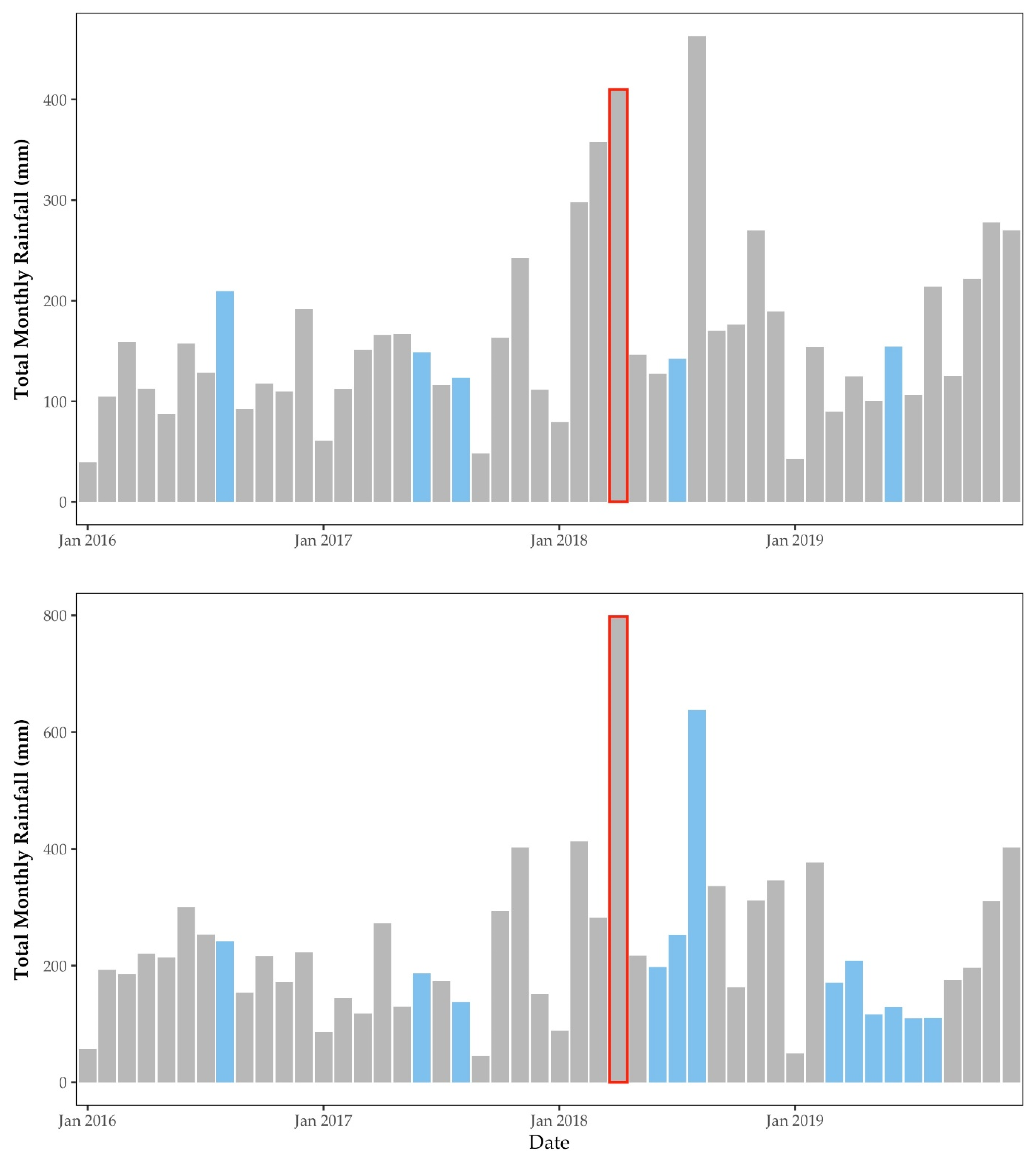
2.4.1. Rainfall

Rainfall data were gathered and utilized to describe the extent of freshwater input into the Pila‘a and Hā‘ena reef sites (Figure 5). Pila‘a total monthly rainfall data (mm) were gathered from the Kilauea rain gauge (SKN: 1134) and Hā‘ena total monthly rainfall data (mm) were gathered from the Wainiha rain gauge (SKN: 1115), each from 2016 to 2019 [6,7,69]. Field measurements of water salinity and pH were not available for this study due to inconsistent site access. Generally, the unpredictable nature of storm events and coastal runoff makes inclusion of these in situ water quality variables into studies investigating flooding incidents difficult. Although both rain gauges were located upstream and at higher elevation than the reefs, our estimates of rainfall do unequivocally show that (a) 2018 had an anomalously high amount of rain month-to-month and as a year overall compared to other years in the study period, and that (b) the existence of a major storm-induced flooding event occurred from 13–15 April 2018, about three months prior to our sampling dates.

2.4.2. Temperature

During 2017 and 2018, Onset water temperature Pro v2 loggers were placed on the reef flat at Pila‘a in a spatially strategic design to encompass temperature differences, taking into account proximity to streams, current wave patterns, and depth (Figure 2). The number of loggers installed and retrieved varied by year as a result of missing loggers or instrument failure (Table 1). In 2017, temperature data were averaged between six loggers in the East and four loggers in the West, and in 2018, temperature values were averaged from four loggers in the East and two loggers in the West. For relocation purposes, wire leader was attached to a small 10 cm float extending approximately 20 cm from the end of a 3/16 inch stainless-steel pin with a stainless-steel cable tie securing each temperature gauge. GPS coordinates were documented for each location using a Garmin GPSmap 78sc. Location selection criteria and spatial distribution were based on depth, coverage, and transect location to allow full spatial representation of the reef flat. Gauges recorded temperature at 30 min intervals throughout the deployment period. Data were downloaded annually using Onset HOBOware version 3.7.12. No temperature data were collected for the Hā‘ena region.

2.4.3. Sediment Characteristics

Sediment Collection

Two replicate bulk sediment samples were collected in Nasco Whirlpak^® 13-ounce bags at each collection location from points stratified by depth using ArcGIS ArcMap 10.3.1 (Figure 2 and Figure 3). At Hā‘ena, sampling occurred during August 2016 and June 2018 and, at Pila‘a, during August 2016 and July 2018. Sediment was collected where available from the substrate surface in closest proximity to the GPS point, with all samples at Hā‘ena taken from <7 m depth and all samples at Pila‘a from <3 m depth. Collection bags were approximately half filled with sediment. Sediment sample sizes from Hā‘ena and Pila‘a are shown in Table 1. All samples were first homogenized with a scoop, with two subsamples then obtained from each of the two replicate samples for subsequent sediment grain size and composition analyses to determine the average proportions in grain sizes and composition for each sampling site.

Sediment Grain Size

To measure size fractions, standard brass sieves were used (USA Standard Testing Sieve, ASTME-11 specifications). A brass catch pan collected the silt/clay fraction. Five size fractions were identified: granule (>2.8 mm), coarse and very coarse sand (500 µm–2.8 mm), medium sand (250–500 µm), fine and very fine sand (63–250 µm), and silt/clay (<63 µm) in accordance with the Wentworth scale [70]. Each size fraction was collected in preweighed Whatman 114 wet-strength filters, air dried and weighed to determine the proportion of each size fraction. Only the four smallest size fractions were used in analyses to avoid overweighting of large pieces.

Sediment Composition

To determine the inorganic–organic carbon fraction, approximately 20 g of bulk sediment were finely ground using an IKA^® A11 basic analytical mill or mortar and pestle. Subsamples were oven-dried for 10 h at 100 °C to remove moisture, placed in a desiccator, and weighed to obtain initial weights. To remove the organic fraction, roughly 10 g were burned in a muffle furnace for 12 h at 500 °C (LOI500), placed in a desiccator, and weighed [71,72]. For removal of carbonate material, samples were placed in a muffle furnace for 2 h at 1000 °C (LOI1000), cooled in a desiccator, and weighed [72]. The remaining sample after initial incinerations represented terrigenous material, and loss-on-ignition values were then used to calculate proportions of each sediment component (organic, carbonate, terrigenous) [72].

2.5. Statistical Analysis

R (Version 3.6.2) and the integrated development environment, R-Studio Desktop (Version 1.1.453, RStudio PBC, Boston, MA, USA), were used for all data analyses [73]. Significance level was set at α = 0.05 for all analyses. Graphs depicting discrete biotic populations (fishes, urchins, and coral) were generated using JMP^® Pro 15 (SAS Institute Inc., Cary, NC, USA).

2.5.1. Environmental Data

Summer temperatures from June through September were isolated in order to examine possible correlation with coral bleaching. In cases where multiple loggers gathered data, temperatures were averaged to evaluate annual differences during summer months. The high level of observed bleaching instigated the calculation of degree heating weeks (DHW) based on the mean monthly maximum and a bleaching threshold of 29 °C. DHWs were used to determine whether elevated temperatures, rather than only salinity decreases, contributed to bleaching [12]. Overall mean summer temperatures during 2017 and 2018 were calculated as grand means taken from the individual monthly means of June through September.

Grain size data for coarse, medium, and fine sand proportions from Pila‘a and Hā‘ena were normalized using a logit transformation and subsequent homogeneity of variance assessed using a Levene’s test from the R package car [74]. Transformed grain size proportions from 2016 and 2018 were then compared by year at Hā‘ena and by sector and year at Pila‘a using unpaired two-tailed t-tests. Silt/clay grain size data and sediment composition data at Pila‘a and Hā‘ena were evaluated using unpaired Wilcoxon rank sum tests, as these data were unable to be normalized. No environmental data were compared between sites.

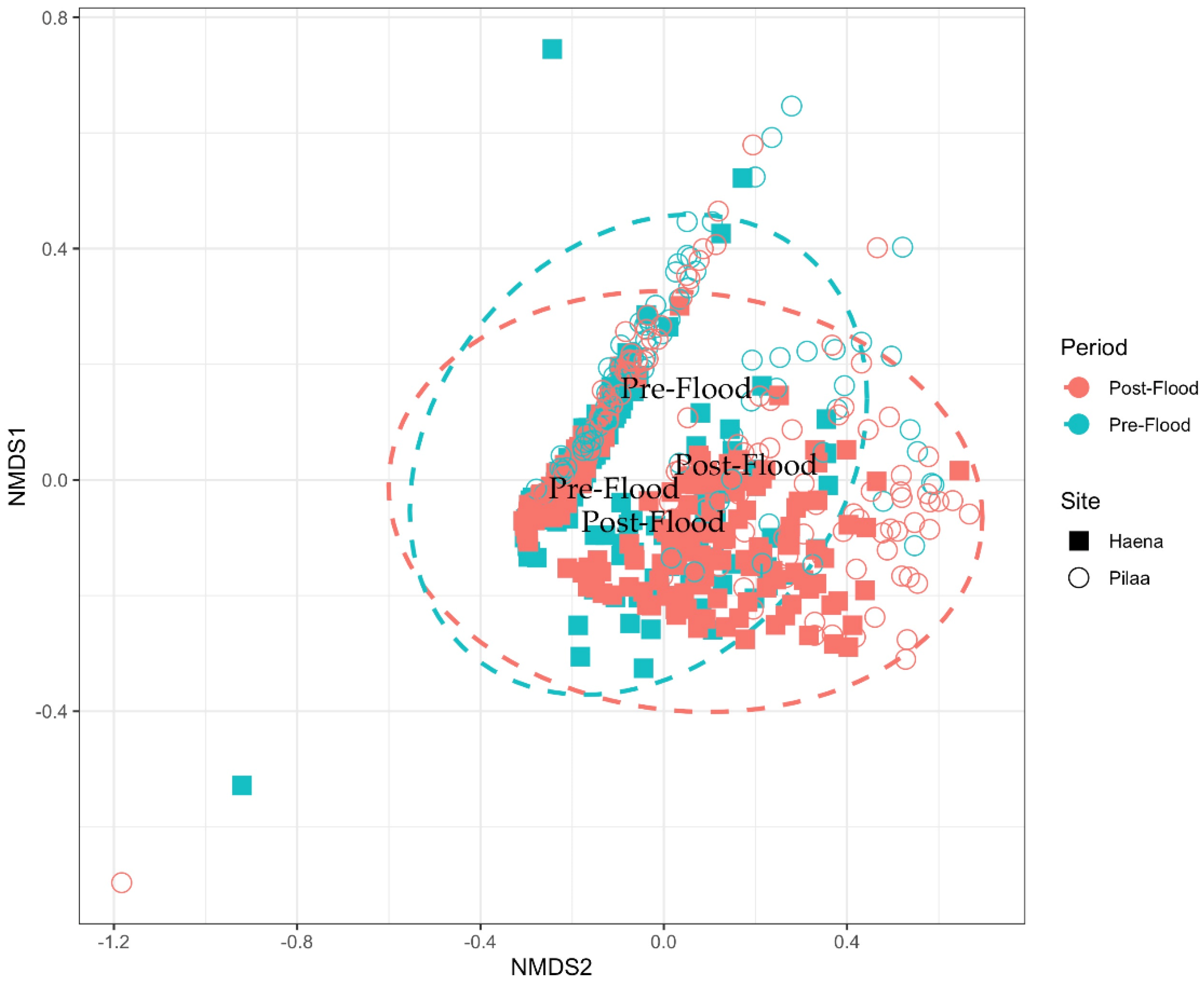
2.5.2. Community-Level Multivariate Approach

All biological data were analyzed at a community level using nonmetric multidimensional scaling (nMDS) models. Variables included in community matrices were fish count, fish diversity, number of fish species, urchin count, and percent bleached coral of total coral cover. Site (Hā‘ena and Pila‘a) and period (pre-flood (2016–2017) and post-flood (2018–2019)) were used as grouping factors. Ecological variables were evaluated between and among sites; a total of three models were used to visualize and interpret dissimilarity in the overall multivariate community responses. For the aggregated model, there were a total of 573 observations, while the Hā‘ena-only model used 380 and the Pila‘a-only model used 193. Input data for multivariate analyses were square-root transformed and a Bray–Curtis index calculated to construct distance matrices for the creation the nMDS plots. All nMDS model were iterated a maximum of 100 times at three dimensions (k = 3). Permutational multivariate analyses of variance (PERMANOVA, [75]) were conducted to determine any effects of reef depth or sector and timing of the flood event on community structure, with number of permutations set at a maximum of 999. Subsequently, pairwise comparisons of the sector/depth and time period were examined using the similarity percentage (SIMPER, [76]) in order to assess the contribution of each biological parameter to the average dissimilarity between groups. Multivariate analyses were performed using the R package vegan [77].

2.5.3. Discrete Population Univariate Approach

Negative binomial generalized linear models (GLM) were applied to analyze the non-normal sea urchin count data at Hā‘ena and Pila‘a using the R package MASS [78]. These best fit GLMs were selected by evaluation of Akaike information criterion (AIC) values, overdispersion indices, and residual plots. Best fit models included interaction terms for both Hā‘ena (Year x Depth) and Pila’a (Year x Sector). Model estimated marginal mean (EMM) contrasts with false discovery rate (FDR) adjustments were used to evaluate post hoc differences in urchin counts between years for a given site. EMM comparisons were completed using the R package emmeans [79]. Separate GLMs were run for Hā‘ena and Pila‘a, as no between site models were created for any biological univariate data (including fish, described below).

Fish counts were modeled at Hā‘ena using a negative binomial GLM, which was selected via the same criteria used for sea urchin counts. The best fit model was found to explain count data interactively (Year x Depth). Model EMM contrasts with FDR adjustments were also used to examine post hoc differences in fish counts between years and depths. Fish biomass data were normalized using a fourth-root transformation and subsequent tests for homogeneity of variance between years and depths confirmed using a Levene’s test. A two-way analysis of variance (ANOVA) with year and depth as factors was then run to assess differences in average biomass with respect to year and depth. Fish abundance and biomass at Pila‘a were not included in univariate analyses.

Overall fish abundance at Hā‘ena was assessed and divided into functional groups of invertivores, herbivores, zooplanktivores, and piscivores. Methodology drew directly from previously analysis of data undergone in Rodgers et al. [57]. Data for each trophic level were evaluated using nonparametric Kruskal–Wallis tests with year as the sole factor, as they were unable to be normalized. Post hoc comparisons by year were completed using Dunn tests with Bonferroni adjustments. Kruskal–Wallace tests were performed using base R and Dunn tests were run using the R package DescTools [80].

The abundance (percent of total coral cover) and distribution of S. edmondsoni were assessed via KAHU surveys at Pila‘a only. The presence of S. edmondsoni was not detected at Pila‘a West and, at Pila‘a East, the distribution of proportion data was non-normal and had predominantly zero values for all years except 2018. As such, yearly S. edmondsoni abundance at Pila‘a East was evaluated via a univariate PERMANOVA with a Euclidean dissimilarity index, with number of permutations set at a maximum of 999 [75,77]. To examine differences in abundance between years, a post hoc analysis was run using the R package pairwiseAdonis [81]. Additionally, the relative occurrence (presence/absence) of S. edmondsoni between years was compared using chi-squared test of proportions.

Proportion of bleached coral was calculated as a percentage of the total observed coral. Bleached coral proportion data were not normally distributed at Hā‘ena and Pila‘a, thus nonparametric unpaired Wilcoxon rank sum tests were used for comparison of bleached coral from 2017 to 2018 at both sites.

3. Results

3.1. Environmental Factors

3.1.1. Rainfall & Temperature

Total monthly rainfall for both study sites is shown in Figure 5. Total rainfall during the study period was highest at Hā‘ena during April 2018 (798 mm) and highest at Pila‘a during August 2018 (463 mm). Although rainfall in Pila‘a was greatest during August 2018, the major pulse event occurred during April 2018, which received a total of 410 mm. Mean total monthly rainfalls at Hā‘ena and Pila‘a during the study period (excluding April 2018) were 216 and 158 mm, respectively.

Temperature data from the summer months (June–September) of 2017 and 2018 were extracted from loggers deployed at Pila‘a East and West, although data from July–September 2017 at Pila‘a East were lost and temperature after July 2018 would not have influenced the coral bleaching surveys presented in this study.

Mean temperatures at Pila‘a East during 2017 and 2018 were 26.6 and 26.7 °C, respectively, with the maximum temperature in 2017 (29.3 °C) being higher than the maximum temperature in 2018 (28.3 °C). A total of 2.5 h of temperatures exceeding the coral bleaching threshold (>29 °C) were recorded during the 2017 summer months, although there were no thermal anomalies above the bleaching threshold during 2018 summer months [12]. Furthermore, mean temperature by month during 2017 and 2018 did not exceed 26.7 °C during any month of 2017 or 2018. Mean temperatures at Pila‘a West during 2017 and 2019 were 27.0 and 26.4 °C, respectively, with similar maximum temperatures during 2017 (28.9 °C) and 2018 (28.7 °C) and no incidences of temperature exceeding the coral bleaching threshold. Mean temperature in 2017 was highest during September (27.6 °C) and, in 2018, during July (26.3 °C). When combining temperature from both sectors, mean summer temperature at the Pila‘a reef was lower in 2018 (26.3 °C), the year of the flood event, than in 2017 (27.1 °C).

3.1.2. Sediment

Pila‘a sediment grain size between years and sectors show an increase in coarse sand and silt/clay fractions from 2016 to 2018 (

Table 2. Mean and ±SE of the mean of sediment grain size fractions (%) at Pila‘a and Hā‘ena during 2016 (pre-flood) and 2018 (post-flood). The shallow Pila‘a reef flat was sampled at 1–2 m, whereas Hā‘ena sediment was sampled at stations <7 m in depth. Significant differences between 2016 and 2018 for a given sector or depth are denoted by * = p ≤ 0.05 or by a trend towards significance ^† = p ≤ 0.1. Differences between years were evaluated using t-tests for coarse, medium, and fine grain sizes, whereas Wilcoxon rank sum tests were used for silt/clay comparisons between years.

Site	Year	Coarse	Medium	Fine	Silt/Clay
Pila‘a East	2016	84.9 ± 4.7	7.9 ± 2.0	6.1 ± 3.4	1.2 ± 0.5
Pila‘a East	2018	65.8 ± 7.9 *	15.0 ± 6.3	9.1 ± 1.1	10.1 ± 0.8 *
Pila‘a West	2016	88.7 ± 2.2	8.6 ± 2.6	2.1 ± 0.5	0.6 ± 0.2
Pila‘a West	2018	65.9 ± 7.5 *	17.0 ± 5.3	8.1 ± 2.3 *	8.9 ± 0.9 †
Hā‘ena	2016	71.6 ± 11.4	17.5 ± 6.0	10.5 ± 6.1	0.4 ± 0.1
Hā‘ena	2018	61.5 ± 5.1	24.7 ± 4.6 †	7.7 ± 1.6	6.2 ± 0.3 *

). The freshwater and sediment input from the major flooding event in 2018 resulted in greater proportions of fine silt/clay and terrigenous deposits on both sectors of the Pila‘a reef as compared to 2016. The level of silt/clay in the East during 2018 (10.1%) was much higher than 2016 levels (1.2%, Table 2), but lower than those reported in 2002 following the 2001 major sediment event (13.9%) that devastated the East Pila‘a reef flat [51]. The increase from 2016 to 2018 of silt/clay fractions in the East was significant (Wilcox test, p = 0.003). A similar increase in the West from 0.6% to 9.0% was also observed (Wilcox test, p = 0.100), with less statistical confidence likely due to a smaller sample size (n = 3, Table 1). Alternatively, larger grain (coarse) sizes in the 2016 survey prior to the flood event were greater in the East (84.3%) and West (88.8%) as compared to post-flood fractions (t-tests, East 65.8%, p = 0.028 and West 65.9%, p = 0.035).

Hā‘ena sediment grain size measurements between years are also shown in Table 2. The fraction of silt/clay increased from 0.4% in 2016 to 6.2% in 2018 (Wilcox test, p ≤ 0.001). Coarse sand also decreased from 71.6% in 2016 to 61.5% in 2018; however, this difference was not statistically significant. Hā‘ena sediment data were only sampled at shallow depths (≤7 m, Figure 3).

Sediment composition (organics, carbonate, and terrigenous) was also analyzed in 2016 and 2018 at both Pila‘a sectors and Hā‘ena shallow stations (not shown). Carbonate was the most dominant sediment type, comprising at least 85% of total sediment across all years and sites. Terrigenous sediment, which is commonly associated with flood runoff, increased from 3.2% in 2016 to 5.5% in 2018 at Pila‘a East, although this was not statistically significant. Alternatively, Pila‘a West terrigenous sediment was mostly unchanged (2.5% in 2016 and 2.3% in 2018). Terrigenous sediment at Hā‘ena decreased from 8.0% in 2016 to 5.9% in 2018, albeit insignificantly. There were no significant changes between years for any sediment types at Pila‘a or Hā‘ena.

3.2. Biological Factors

3.2.1. Community-Level Changes

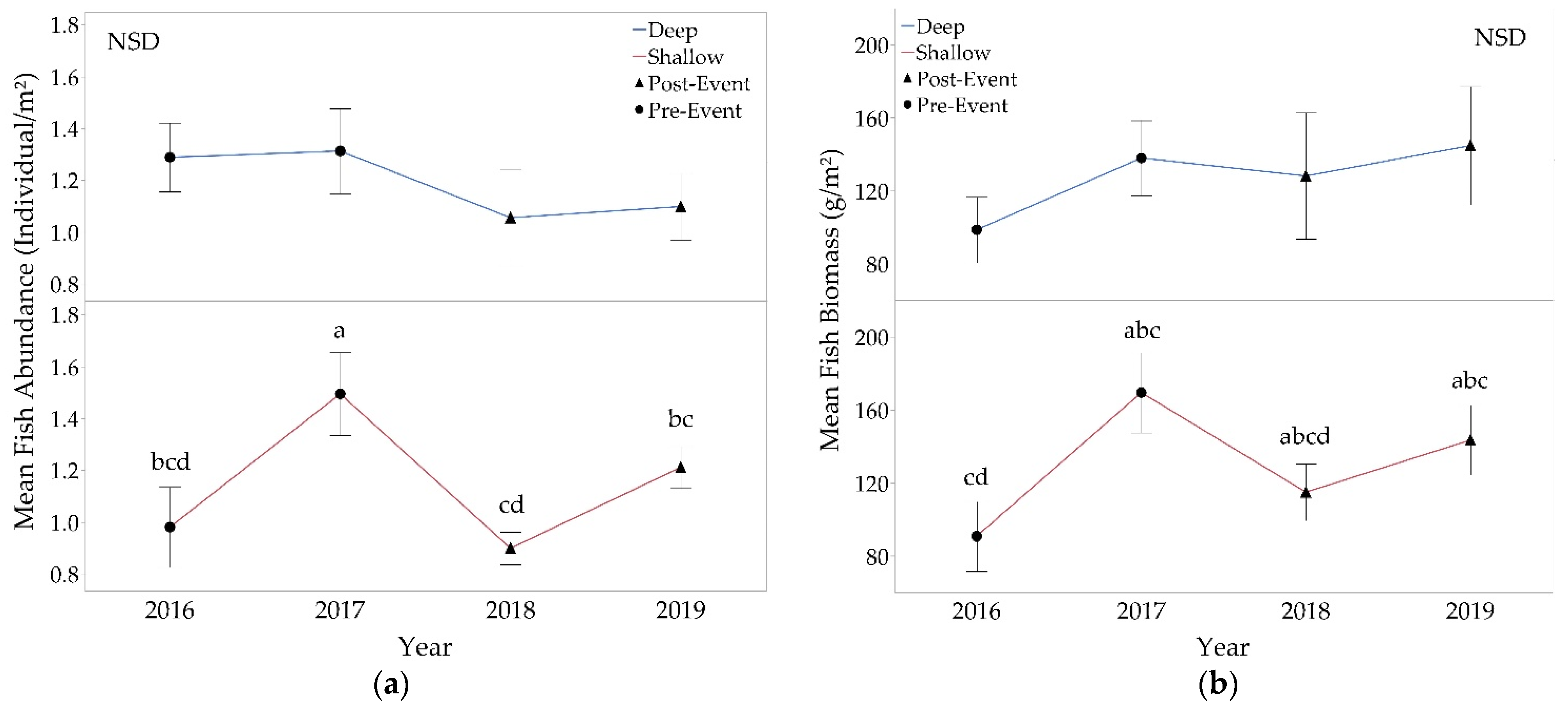
The multisite nMDS model successfully converged and well represented characteristics of reef organism assemblage that may be influenced by site and period (stress = 0.05, nonmetric fit R² = 0.99). Figure 6 shows a slight deviation in reef community characteristics before and after the flood event in April 2018 at both Hā‘ena and Pila‘a.

PERMANOVA results indicated that there were differences in the positions of surveyed transects in multivariate space when compared by site (df = 1, p = 0.001) and period (df = 1, p = 0.001). The interaction between location and period was also significant (df = 1, p = 0.017). There were differences in how reef organisms responded at Hā‘ena and Pila‘a before and after the flood event. Pairwise comparisons showed that fish count (p = 0.001) contributed to the dissimilarity between pre- and post-flood event periods at Hā‘ena. At Pila‘a, biological variables contributing to the dissimilarity between the pre- and post-flood reef communities included bleached corals (p = 0.001), fish diversity (p = 0.009), and number of fish species (p = 0.012). When comparing community differences between Hā‘ena and Pila‘a, pairwise comparisons also indicated that fish count (p = 0.036) contributed to the dissimilarity between the two sites prior to the flood event. After the flood event, sea urchin count (p = 0.001) and bleached coral (p = 0.001) contributed to the dissimilarity in reef community characteristics between the two sites.

When evaluating community shifts at Hā‘ena only, the nMDS model converged resulting in a strong representation of the biological community (stress = 0.06, nonmetric fit R² = 0.99). PERMANOVA results showed a difference among groups when compared by depth (df = 1, p = 0.001) and period (df = 1, p = 0.001), whereas the interaction between depth and period was not significant. Pairwise comparisons showed that fish count (p = 0.001), fish diversity (p = 0.002), and sea urchin count (p = 0.049) contributed to the dissimilarity between pre- and post-flood communities in the shallow sector. In the deep sector, no specific biological factors contributed to the dissimilarity between flooding periods. Fish count (p = 0.002) and sea urchin count (p = 0.043) contributed to the dissimilarity between the shallow and deep sectors before the flood, while bleached corals explained dissimilarity (p = 0.001) between the shallow and deep groups after the flood event.

The nMDS model for Pila‘a also converged and well represented the responses of reef organisms (stress = 0.05, nonmetric fit R² = 0.99). PERMANOVA results showed that there were differences in groups compared by sector (df = 1, p = 0.001) and period (df = 1, p = 0.001). The interaction between sector and period was also significant (df = 1, p = 0.017). Pairwise comparisons showed that number of fish species (p = 0.001) contributed to the dissimilarity between pre- and post-flood event groups in the East. In the West, no specific biological factor contributed to the dissimilarity between pre- and post-flood groups. While the fish count (p = 0.047) and sea urchin count (p = 0.001) contributed to the dissimilarity between the East and West sectors before the flood, bleached corals contributed to the dissimilarity (p = 0.001) between the East and West sectors post-flood event.

3.2.2. Fishes

Changes in total fish populations were calculated at Hā‘ena. A large percent change in mean total fish abundance (−32.7%) and biomass (−22.9%) was observed from 2017 to 2018, with a contrasting increase from 2018 to 2019 in abundance (+22.7%) and biomass (+20.8%). With respect to abundance, this decrease from 2017 to 2018 was significant (EMM, p ≤ 0.001), however, the subsequent recovery in 2019 was not. These declines in total abundance from 2017 to 2018 were consistent when fish populations were grouped by trophic level (not shown, [57]). Decreases in mean invertivore (−21.4%) and zooplanktivore (−73.0%) abundance occurred from 2017 to 2018 (Dunn, p = 0.014 and p ≤ 0.001, respectively). A decrease in mean herbivore abundance (−30.0%) was also observed, although this change was insignificant (Dunn, p = 0.314). There was no observed change in average piscivore abundance, although in both 2017 and 2018 this trophic level accounted for only 2.74% of total fish abundance.

Year and depth were found to interactively explain differences in fish abundance (LR χ² = 8.11, df = 3, p = 0.044). Similar patterns to those seen for overall abundance were found at shallow stations only (≤7 m), showing a pronounced decline in fish abundance from 2017 to 2018 (EEM, p ≤ 0.001, Figure 7a,

Table 3. Model estimated marginal mean (EMM) post hoc comparisons of fish abundance at Hā‘ena between years separated by depth. Test statistic ratios (z-ratios) represent magnitude of difference, with a positive ratio indicating that the left comparison year was greater (and vice versa). Bolded and italic comparisons represent a significant difference * = p ≤ 0.05 or a trend towards a significance difference ^† = p ≤ 0.1.

Depth	Years	Z-Ratio	SE	Sig.
Shallow	2016–2017	−3.548	0.085	0.001 *
	2016–2018	0.380	0.155	0.704
	2016–2019	−1.412	0.122	0.189
	2017–2018	4.566	0.209	<0.001 *
	2017–2019	2.244	0.167	0.050 *
	2018–2019	−2.012	0.102	0.066†
Deep	2016–2017	0.034	0.120	0.973
	2016–2018	1.703	0.195	0.265
	2016–2019	0.970	0.179	0.498
	2017–2018	1.918	0.170	0.265
	2017–2019	1.073	0.157	0.498
	2018–2019	−0.658	0.147	0.612

). There were, however, no changes in abundance at deep stations (>7 m). Although fish biomass declined the year of the flood event at both shallow and deep stations and rebounded the following year, these changes were not statistically significant (Figure 7b).

3.2.3. Sea Urchins

Echinometra mathaei (rock boring urchin) was the dominant sea urchin species found across all years, sectors, and depths. This species accounted for >90% of urchin composition at Pila‘a across all years and sectors, and >50% of urchin composition across all years and depths at Hā‘ena. Total urchin abundance at Pila‘a was influenced by both year (LR χ² = 16.36, df = 3, p ≤ 0.001) and sector (LR χ² = 11.48, df = 1, p ≤ 0.001) without significant interaction. Urchin abundance in East Pila‘a increased from 2016 to 2017 (EMM, p ≤ 0.001), then showed a trend towards a significant decrease from 2017 to 2018 (EMM, p = 0.063). All post hoc comparisons between years, separated by sector, are shown in

Table 4. Model estimated marginal mean (EMM) post hoc comparisons of urchin abundance at Pila‘a (left) and Hā‘ena (right) between years. Test statistic ratios (z-ratios) represent magnitude of difference, with a positive ratio indicating that the left comparison year was greater (and vice versa). Bolded and * comparisons represent a significant difference of p ≤ 0.05, while ^† represent a trend towards significance (p ≤ 0.1).

Sector	Years	SE	z-Ratio	Sig.	Depth	Years	SE	z-Ratio	Sig.
East	2016–2017	0.094	−3.760	<0.001 *	Shallow	2016–2017	0.364	0.741	0.550
	2016–2018	0.178	−1.796	0.109		2016–2018	1.035	4.524	<0.001 *
	2016–2019	0.210	−1.475	0.168		2016–2019	0.938	3.860	<0.001 *
	2017–2018	0.664	2.307	0.063†		2017–2018	0.737	4.255	<0.001 *
	2017–2019	0.779	2.149	0.063†		2017–2019	0.676	3.500	<0.001 *
	2018–2019	0.342	0.116	0.908		2018–2019	0.224	−0.548	0.584
West	2016–2017	0.295	−0.840	0.481	Deep	2016–2017	0.211	−1.029	0.495
	2016–2018	0.452	0.077	0.939		2016–2018	0.235	−0.882	0.495
	2016–2019	0.690	1.192	0.430		2016–2019	0.386	0.819	0.495
	2017–2018	0.534	1.065	0.430		2017–2018	0.306	0.061	0.952
	2017–2019	0.799	2.502	0.074†		2017–2019	0.503	1.827	0.313
	2018–2019	0.576	1.289	0.430		2018–2019	0.536	1.625	0.313

.

Year and depth were found to interactively explain changes in Hā‘ena urchin abundance (χ² = 15.58, df = 3, p = 0.001, Figure 8a). There were no significant differences in urchin abundances between years at deep stations (>7 m). At shallow stations, however, urchin abundance during 2017 was greater than urchin abundance during 2018 (EMM, p ≤ 0.001). All post hoc comparisons between years, separated by depth, are shown in Table 4.

3.2.4. Sarcothelia Edmondsoni

The abundance and distribution of the zooxanthellate soft octocoral Sarcothelia edmondsoni showed marked increases following the flood event in 2018 at Pila‘a. S. edmondsoni was recorded on 4% of the KAHU transects in 2016 (n = 50), 0% in 2017 (n = 51), 15% in 2018 (n = 50), and 0% in 2019 (n = 50). The presence of S. edmondsoni was not detected through KAHU transect surveys at Pila‘a West during any of the study period years. At Pila‘a East, the proportion of transects where presence of S. edmondsoni was observed was highest during 2018 when compared to all other years (χ², p ≤ 0.05 for all comparisons).

The percent of total coral cover for S. edmondsoni at Pila‘a East differed by year (PERMANOVA, p = 0.003, Figure 9). S. edmondsoni abundance was highest during 2018 when compared to all other years (p ≤ 0.05,

Table 5. Pairwise PERMANOVA post hoc comparisons of S. edmondsoni abundance at Pila‘a East between years. Bolded and * comparisons represent a significant difference of p ≤ 0.05.

Sector	Years	F	Sig.
	2016–2017	0.921	0.755
	2016–2018	3.872	0.045 *
East	2016–2019	0.847	0.758
	2017–2018	4.967	0.023 *
	2017–2019	N/A	N/A
	2018–2019	4.565	0.031 *

).

Detailed benthic mapping surveys initiated in 2018 and continued in 2019 show similar results as the benthic KAHU surveys for recovery following the flood. The distribution of S. edmondsoni was considerably more extensive following the flood in 2018 than one year later in 2019, showing a 41.8% decline in distribution (Figure 10).

3.2.5. Coral Cover & Bleaching

Mean coral cover at Pila‘a was notably lower than the state average for the Main Hawaiian Islands and was relatively consistent from 2016–2019, ranging from 2.1% to 2.7% as compared to the state average of 20.8% [82]. Dominant corals included Porites lobata, P. compressa, Pocillopora meandrina, Montipora capitata, M. patula, and the octocoral S. edmondsoni. On the Pila‘a East reef flat, mean bleached coral was lower in 2017 (10.7%) than in 2018 (23.5%), although this change was not statistically significant likely due to the high number of zero values and variability (Wilcox, p = 0.133, see Figure S3a). On the Pila‘a West reef flat, mean bleached coral percentages were similar in 2017 (14.8%) and 2018 (13.8%). In 2017, levels of bleaching were similar in the East and West sectors, while in 2018 bleached coral percentage was notably higher in the East than in the West, albeit statistically insignificant. M. capitata was the most common bleached coral species found in Pila‘a.

At Hā‘ena, mean coral cover ranged from 4.9% to 6.2% between 2016–2019, with P. lobata, M. patula, and P. meandrina comprising the most dominant corals. At deep stations, mean bleached coral increased from 5.5% in 2017 to 12.9% in 2018 (Wilcox, p = 0.043, see Figure S3b). Mean bleached coral also increased at Hā‘ena shallow stations from 2.8% in 2017 to 4.5% in 2018, although the change was not statistically significant (Wilcox, p = 0.144). Bleaching at deep stations trended towards being greater than bleaching at shallow stations during 2017 (Wilcox, p = 0.093), with bleaching also being higher at deep stations in 2018 (Wilcox, p = 0.010). M. capitata and M. patula were the most common bleached coral species found at Hā‘ena.

The unintuitive higher bleaching at deep stations prompted an examination of the genus Montipora, which generally has particularly high cover [83] and one of the lowest thermal tolerances in Hawai‘i [20]. Montipora capitata, M. patula, and M. flabellata were collectively examined for bleaching differences between deep and shallow stations in 2018, the year of the flood. Total coral cover of these species was not significantly different between shallow (58.2%) and deep stations (53.4%), although the percent of bleaching was highest among the Montiporids in deeper waters.

4. Discussion

The outcomes of our study unequivocally show that the April 2018 historic flood event on the north shore of Kaua‘i had a deleterious effect on the Pila‘a and Hā‘ena reef communities and their individual populations. Community models combining fish, urchin, and coral bleaching factors showed significant shifts in community structure before and after the storm event at both Pila‘a and Hā‘ena (Figure 6). In tandem with community changes, our univariate models showed significant declines in shallow and overall fish populations at Hā‘ena, suggesting flooding inputs were concentrated at shallow sites. There was also evidence showing coral bleaching increased following the flood event, despite temperatures consistently being recorded within the range of coral tolerance. Indeed, species-specific bleaching following this flood event were consistent with statewide patterns from temperature-related bleaching [24,84], with corals in the genus Montipora and Pocillopora exhibiting the lowest tolerance to salinity. We also observed a major population increase in the octocoral Sarcothelia edmondsoni after the storm event, followed by subsequent declines in 2019, suggesting that S. edmondsoni is relatively resilient to low salinities and may act a bioindicator of freshwater input. Lastly, we recorded marked declines in the abundance of the dominant urchin species, E. mathaei, in the inundation-prone shallow waters of both sites.

Proportional shifts between larger grain size and silt/clay fractions can be indicative of heavy sedimentation, which is common after major flooding events [85,86]. These trends are consistent with observations at Pila’a East, where large grain sediment decreased and silt/clay increased from 2016 to 2018 (Table 1). Additionally, the lower levels of small grain sizes, organics, and silt/clay deposits on Pila‘a West, where stream input is more restricted, providing supporting evidence for the expectation of greater sedimentation impacts to Pila’a East. At Hā‘ena, the increase in silt/clay levels during 2018 also suggests flooding-associated sedimentation at shallow stations. Sediment data were not collected at deep stations, however, and the decrease in fine-grained and terrigenous sediment are not consistent with expected outcomes. This is likely due to the relatively high circulation and mixing in Hā‘ena waters [87] relative to the Pila‘a system, which may have resuspended and advected sediments between the flood event and sampling. According to the wave observation buoy data at Hanalei, there was a high wave event with the maximum height of 4.9 m and swell periods of 12–13 s on 29–30 April from the north direction. Hā‘ena is located approximately 6.5 km west of Hanalei, and greater water motion and mixing on Hā‘ena reefs is expected as they face directly north. Additionally, the range of shallow transect distances from shore is much greater at Hā‘ena (Figure 3), which may have led to freshwater dissipation and dilution before interaction with farther offshore transects.

The results of our rainfall and sediment data should allow for reasonable confidence in the statistical and inferential association between certain population shifts and the major flooding event. Sediment can play an important role in determining the condition or state of the reefs as, when silt and clay overwhelm reef systems, sedimentation becomes the dominant forcing function on community structure [83]. However, this study did not separate the effects of freshwater from the effects of sediment input. Declines in benthic populations and fishes may have been attributed to lower salinities and increased sedimentation individually or synergistically.

4.1. Fish Populations

The April 2018 freshwater event likely contributed to the notable declines in overall and shallow fish abundance and biomass in 2018. Supporting evidence of this interpretation comes from the observed depth-specific changes, as fish populations post-flooding decreased at shallow stations closer to freshwater input. There were, however, no differences found at deep stations further removed from the coastline. Pairwise findings from PERMANOVA affirm these univariate findings, as fish count and diversity contributed to the dissimilarity between shallow water communities before and after the flood, which was not the case for deep waters. Overall, fish populations increased in the year prior to the flood (2017), most likely due to implementation of fishing regulations, then declined in the year of the flood (2018), ultimately rebounding in 2019 (Figure 7a) [50,57,63,64].

In the 1980s, a large storm event on Kona, Hawai‘i, resulted in declines of many reef fish taxa in shallow areas, but not deeper zones, consistent with our findings here [43]. At Hā‘ena, decreases in fish populations occurred across each trophic level, suggesting that resultant changes to the reef were pervasive. Although the exact cause of the observed deteriorations in fish populations is ambiguous, our data do show clear evidence of nontransient declines in fish abundance after a flood event. These declines, however, were followed by partial rebounds of overall fish populations in 2019 (Figure 7). As was also seen in population increases from 2016 to 2017, this growth is likely attributed to the effectiveness of the fishing reserve [57].

4.2. Sea Urchin Populations

Significant declines in urchin abundance were observed at the shallow transects of both sites with no concurrent decreases in deep water populations, where a lower likelihood of freshwater contact occurs. E. mathaei, the dominant urchin species at Hā‘ena and Pila‘a, appeared to be the most heavily impacted by freshwater. At Hā‘ena, E. mathaei declined at shallow stations from 2017 (7.7 urchins/transect) to 2018 (1.1 urchins/transect); however, at deep stations there was no change in urchin abundance, providing strong evidence of freshwater impacts (Figure 8b). These findings were consistent with pairwise PERMANOVA results, which found that sea urchin count contributed to the dissimilarity in community structure at shallow sites before and after the flood.

Similar to shallow Hā‘ena areas, the relatively exposed East Pila‘a reef flat showed declines in sea urchin abundance while the West, which is less susceptible to freshwater influence, did not (Figure 8a). These findings further support the classification of freshwater or sediment inputs as drivers of declines in urchin populations and imply the potential of E. mathaei as a proxy or indicator of freshwater impacts. Adult and larval echinoderms have been well documented to be stenohaline, able to tolerate only a narrow range of salinities [88]. This is due to their permeable body wall [89] and lack of separated osmoregulatory and excretory organs [90]. Other possible explanations for the pronounced decline in urchin populations include elevated sedimentation and pollutive nutrient levels associated with the flood runoff. Sediment with <63 μm grain size has been shown to reduce larval settlement, recruitment, and survivorship of juvenile sea urchins [91]. Finer grain size fractions, which have high surface area relative to their volume, are more susceptible to bonding with organic compounds and/or pollutants than larger grain sizes; for example, the concentration of organic carbon in the silt/clay fraction of fluvial bed sediment from Mānoa Stream, O‘ahu, was 4.6 times higher than in its coarse sand fractions [92]. Sea urchin gametes are commonly used in toxicity bioassays due to their sensitivity to environmental pollutants [93], where fertilization success has been shown to decline with increases in sediment toxicity [94].

4.3. Coral

4.3.1. Octocoral Sarcothelia edmondsoni

Supporting evidence of the major flooding event’s impact is shown by the dramatic, significant shift in the abundance of the octocoral, Sarcothelia edmondsoni (Figure 9 and Figure 10), before and after the flood at Pila‘a. In 2018, S. edmondsoni area of cover and frequency of occurrence on transects was highly evident at Pila‘a East, the area more heavily impacted by freshwater, while the octocoral was nearly absent prior to the flood in the East and throughout all years surveyed in the West. Additional mapping surveys also showed a subsequent drop in cover the year following the flood; however, in contrast to the transect surveys that detected no S. edmondsoni (0%) in 2019, the octocoral still showed a notable presence at Pila‘a East.

The results of this study lend preliminary support to the novel classification of the soft coral S. edmondsoni as a potential bioindicator of freshwater input. Several studies have elucidated the prospect of octocorals to act as bioindicators of various natural and anthropogenic reef inputs [60,61], but presently there exists little nonanecdotal evidence to support these findings regarding S. edmondsoni and freshwater in the Hawaiian Islands.

4.3.2. Coral Bleaching

Despite temperatures consistently staying below coral bleaching thresholds prior to and during the year of the flood, coral bleaching was higher following the flood than in previous years at both sites. A change in environmental conditions outside coral thresholds can cause bleaching (i.e., temperature, nutrients, salinity, sedimentation, exposure) [24]. Jokiel and Coles [24] determined the bleaching threshold for Hawaiian corals at 29–30 °C, which is 1–2 °C greater than the observed upper summer maximums at Pila‘a. Despite this, there was an increase in coral bleaching at the flood-impacted Pila‘a East during 2018. Temperature stress was eliminated as the cause of bleaching at Pila‘a, as loggers did not record temperatures outside coral thermal tolerances for any extended period, and no widespread bleaching was observed during 2018 throughout the rest of the Hawaiian Islands. The observed bleaching at Pila‘a was likely attributed to the unprecedented flooding that exposed corals to extensive freshwater. The eastern reef saw immediate evidence of bleaching, while the western reef, with lower freshwater influence, was less impacted. Sedimentation may also have contributed to higher bleaching after flooding as silt/clay sized sediment has longer settling time and resuspension in water column, affecting turbidity and altering quantity and quality of irradiance [95,96,97]. Additionally, the removal of deposited fine and silt/clay size sediment by corals is less efficient than the removal of larger, coarse grain size sediment, suggesting high energetic cost for expulsion [85]. The adverse impacts of turbidity and direct sediment deposition on adults, reproduction, and early life history of symbiotic corals have been well documented and reviewed extensively (e.g., [98,99]). Alternatively, factors associated with storm inputs that can instead ameliorate bleaching include suspended sediments and plankton growth, which can lessen irradiance levels to corals and thus reduce temperature from increased circulation and mixing. These factors may have mediated the levels of bleaching found in this study.

Although coral bleaching was higher at both shallow and deep stations at Hā‘ena in the year of the flood event (2018) as compared to the previous year (2017), a statistical difference between years was only found at the deeper stations. The combination of a lack of temperature data and higher bleaching at deeper sites excludes an empirical correlation between coral bleaching and the flood event at Hā‘ena. Bleaching in the Hawaiian Islands has consistently been reported to be significantly higher in shallow waters, although bleaching has also been reported at deep sites [100]. Historically, it has been assumed that coral bleaching is mitigated in deeper waters, relating to the cooler temperatures, and may serve as a reserve for shallow coral restoration [101]. More recent research, however, has shown extensive bleaching at deeper reefs [102], even into the mesophotic zone at up to 60 m depth [103,104]. Explanations clarifying this counterintuitive inconsistency include tidal mixing with shallow heated waters [105], anomalous deep-water currents [102], host nutrient starvation [103], and the possible predominance of more stress-tolerant corals at shallow sites [29,106]. Corals live within 1–2 °C of their upper thermal limits [24]; adaptation to cooler temperatures, geographically and at depth, reduces the thermal threshold of corals, predisposing them to bleaching and allowing for higher susceptibility to fluctuating temperatures than corals in shallow or warm water regions [12,107].

4.4. Management Implications

As storm frequency and intensity increase locally and globally [4,5] and nearshore land use shifts towards more nonpermeable surfaces [30,108], there will be indefinite increases in freshwater, sediment, and nutrient inputs into reef systems. Data on the severity and intensity of impacts to reefs from freshwater events can assist local management in strategic design and solution development for conservation, restoration, and oftentimes any accompanying legislative measures. Freshwater bioindicator taxa, such as sea urchins and octocorals, can serve as reliable early warning tools or proxies for a reef’s exposure to freshwater. Bioindicators also represent a cost-effective alternative technique to the slower and relatively expensive process of continuous water quality sampling and benthic monitoring.

The majority of Hawai‘i federal and state agencies have policies concerning sedimentation and flooding, basing these policies on scientific research. Effects of sediment to shorelines and coral reef communities is a key priority for many principal management agencies working in Hawai‘i that base management decisions and legislative action on internal and external research regarding sedimentation, erosion, and flooding [109].

As shown in this study, other climate change-induced environmental impacts alongside temperature are major threats to reefs and the other biota they facilitate. Along with temperature increases, freshwater, sediment, and nutrient pulses can also be destructive to coral reef communities and several keystone taxa. Although many coral populations can partially recover from large flood events [19], the frequency and intensity of major weather events are increasing [6,7]. Based on data from the year following the flood and a history of recovery from other environmental stressors, we predict these populations may moderately recover [55,57]. Nonetheless, these precarious local trends, which are only amplified by climate change, further emphasize the urgency to discern how flooding holistically affects reef ecosystems and their important benthic populations.

References

1. Hoegh-Guldberg, O. Climate change, coral bleaching and the future of the world’s coral reefs. Mar. Freshw. Res. 1999, 50, 839–866. [Google Scholar] [CrossRef] [Green Version]
2. Burke, L.; Reytar, K.; Spalding, M.; Perry, A. Reefs at Risk Revisited; World Resources Institute: Washington, DC, USA, 2011. [Google Scholar]
3. Easterling, D.R. Climate extremes: Observations, modeling, and impacts. Science 2000, 289, 2068–2074. [Google Scholar] [CrossRef] [Green Version]
4. Karl, T.R.; Melillo, J.M.; Peterson, T.C.; Hassol, S.J. Global Climate Change Impacts in the United States; Cambridge University Press: New York, NY, USA, 2009. [Google Scholar]
5. Mora, C.; Frazier, A.G.; Longman, R.J.; Dacks, R.S.; Walton, M.M.; Tong, E.J.; Sanchez, J.J.; Kaiser, L.R.; Stender, Y.O.; Anderson, J.M.; et al. The projected timing of climate departure from recent variability. Nature 2013, 502, 183–187. [Google Scholar] [CrossRef] [PubMed]
6. Giambelluca, T.W.; Chen, Q.; Frazier, A.G.; Price, J.; Chen, Y.-L.; Chu, P.-S.; Eischeid, J.; Delparte, D. Online rainfall atlas of Hawai’i. Bull. Am. Meteorol. Soc. 2013, 94, 313–316. [Google Scholar] [CrossRef]
7. Longman, R.J.; Newman, A.J.; Giambelluca, T.W.; Lucas, M. Characterizing the uncertainty and assessing the value of gap-filled daily rainfall data in Hawai‘i. J. Appl. Meteorol. Climatol. 2020, 59, 1261–1276. [Google Scholar] [CrossRef]
8. Jokiel, P. Impact of storm waves and storm floods on Hawaiian reefs. In Proceedings of the Tenth International Coral Reef Symposium, Okinawa, Japan, 28 June–2 July 2004; pp. 390–398. [Google Scholar]
9. Andersson, A.J.; Kuffner, I.B.; Mackenzie, F.T.; Jokiel, P.L.; Rodgers, K.S.; Tan, A. Net loss of CaCO3 from a subtropical calcifying community due to seawater acidification: Mesocosm-scale experimental evidence. Biogeosciences 2009, 6, 1811–1823. [Google Scholar] [CrossRef] [Green Version]
10. Jokiel, P.L.; Bahr, K.D.; Rodgers, K. Synergistic Impacts of Global Warming and Ocean Acidification on Coral Reefs; Pacific Islands Climate Change Cooperative Final Report: Honolulu, Hawai‘i, 2013; p. 63. [Google Scholar]
11. Bahr, K.D.; Rodgers, K.S.; Jokiel, P.L. Ocean warming drives decline in coral metabolism while acidification highlights species-specific responses. Mar. Biol. Res. 2018, 14, 924–935. [Google Scholar] [CrossRef]
12. Jokiel, P.L.; Coles, S.L. Response of Hawaiian and other Indo-Pacific reef corals to elevated temperature. Coral Reefs 1990, 8, 155–162. [Google Scholar] [CrossRef]
13. Jokiel, P.L. Temperature stress and coral bleaching. In Coral Health and Disease; Rosenberg, E., Loya, Y., Eds.; Springer: Berlin/Heidelberg, Germany, 2004; pp. 401–425. [Google Scholar]
14. Hughes, T.P.; Kerry, J.T.; Álvarez-Noriega, M.; Álvarez-Romero, J.G.; Anderson, K.D.; Baird, A.H.; Babcock, R.C.; Beger, M.; Bellwood, D.R.; Berkelmans, R.; et al. Global warming and recurrent mass bleaching of corals. Nature 2017, 543, 373–377. [Google Scholar] [CrossRef]
15. Ward, S.; Harrison, P.; Hoegh-Guldberg, O. Coral bleaching reduces reproduction of scleractinian corals and increases susceptibility to future stress. In Proceedings of the Ninth International Coral Reef Symposium, Bali, Indonesia, 23–27 October 2000; pp. 1123–1128. [Google Scholar]
16. Bahr, K.D.; Jokiel, P.L.; Rodgers, K.S. The 2014 coral bleaching and freshwater flood events in Kāne‘ohe Bay, Hawai‘i. PeerJ 2015, 3, e1136. [Google Scholar] [CrossRef] [PubMed] [Green Version]
17. Banner, A.H. A Fresh-Water “Kill” on the Coral Reefs of Hawaii; Hawai‘i Institute of Marine Biology, University of Hawai‘i: Kāne‘ohe, HI, USA, 1968. [Google Scholar]
18. Jones, A.M.; Berkelmans, R. Flood impacts in Keppel Bay, Southern Great Barrier Reef in the aftermath of cyclonic rainfall. PLoS ONE 2014, 9, e84739. [Google Scholar] [CrossRef]
19. Jokiel, P.L.; Hunter, C.L.; Taguchi, S.; Watarai, L. Ecological impact of a fresh-water “reef kill” in Kaneohe Bay, Oahu, Hawai‘i. Coral Reefs 1993, 12, 177–184. [Google Scholar] [CrossRef]
20. Mayfield, A.B.; Gates, R.D. Osmoregulation in anthozoan–dinoflagellate symbiosis. Comp. Biochem. Physiol. A. Mol. Integr. Physiol. 2007, 147, 1–10. [Google Scholar] [CrossRef] [PubMed]
21. Edmunds, P.; Grey, S.C. The effects of storms, heavy rain, and sedimentation on the shallow coral reefs of St. John, US Virgin Islands. Hydrobiologia 2014, 734. [Google Scholar] [CrossRef]
22. Sheridan, C.; Grosjean, P.; Leblud, J.; Palmer, C.; Kushmaro, A.; Eeckhaut, I. Sedimentation rapidly induces an immune response and depletes energy stores in a hard coral. Coral Reefs 2014, 33, 1067–1076. [Google Scholar] [CrossRef]
23. Bessell-Browne, P.; Negri, A.P.; Fisher, R.; Clode, P.L.; Duckworth, A.; Jones, R. Impacts of turbidity on corals: The relative importance of light limitation and suspended sediments. Mar. Pollut. Bull. 2017, 117, 161–170. [Google Scholar] [CrossRef]
24. Jokiel, P.L.; Coles, S.L. Effects of temperature on the mortality and growth of Hawaiian reef corals. Mar. Biol. 1977, 43, 201–208. [Google Scholar] [CrossRef]
25. Coles, S.; Jokiel, P.L. Synergistic effects of temperature, salinity and light on the hermatypic coral Montipora verrucosa. Mar. Biol. 1978, 49, 187–195. [Google Scholar] [CrossRef]
26. Hoegh-Guldberg, O.; Smith, G.J. The effect of sudden changes in temperature, light and salinity on the population density and export of zooxanthellae from the reef corals Stylophora pistillata Esper and Seriatopora hystrix Dana. J. Exp. Mar. Biol. Ecol. 1989, 129, 279–303. [Google Scholar] [CrossRef]
27. Goenaga, C.; Canals, M. Island-wide coral bleaching in Puerto Rico. Caribb. J. Sci. 1990, 26, 171–175. [Google Scholar]
28. Brown, B.; Dunne, R.; Ambarsari, I.; Le Tissier, M.; Satapoomin, U. Seasonal fluctuations in environmental factors and variations in symbiotic algae and chlorophyll pigments in four Indo-Pacific coral species. Mar. Ecol. Prog. Ser. 1999, 191, 53–69. [Google Scholar] [CrossRef] [Green Version]
29. Cleary, D.F.R.; Polónia, A.R.; Renema, W.; Hoeksema, B.W.; Rachello-Dolmen, P.G.; Moolenbeek, R.G.; Budiyanto, A.; Yahmantoro; Tuti, Y.; Giyanto; et al. Variation in the composition of corals, fishes, sponges, echinoderms, ascidians, molluscs, foraminifera and macroalgae across a pronounced in-to-offshore environmental gradient in the Jakarta Bay–Thousand Islands coral reef complex. Mar. Pollut. Bull. 2016, 110, 701–717. [Google Scholar] [CrossRef] [PubMed]
30. Polónia, A.R.; Cleary, D.F.R.; de Voogd, N.J.; Renema, W.; Hoeksema, B.W.; Martins, A.; Gomes, N.C.M. Habitat and water quality variables as predictors of community composition in an Indonesian coral reef: A multi-taxon study in the Spermonde Archipelago. Sci. Total Environ. 2015, 537, 139–151. [Google Scholar] [CrossRef] [PubMed]
31. Campbell, J.; Russell, M. Acclimation and growth response of the green sea urchin Strongylocentrotus droebachiensis to fluctuating salinity. In Proceedings of the International Conference on Sea Urchin Fisheries and Aquaculture, Puerto Varas, Chile, 25–27 March 2003; pp. 110–117. [Google Scholar]
32. Tsuchiya, M.; Lirdwitayapasit, T. Distribution of intertidal animals on rocky shores of the Sichang Islands, the Gulf of Thailand. Galaxea 1986, 5, 15–25. [Google Scholar]
33. Hughes, T.P. Catastrophes, phase shifts, and large-scale degradation of a Caribbean coral reef. Science 1994, 265, 1547–1551. [Google Scholar] [CrossRef] [PubMed] [Green Version]
34. Lirman, D. Competition between macroalgae and corals: Effects of herbivore exclusion and increased algal biomass on coral survivorship and growth. Coral Reefs 2001, 19, 392–399. [Google Scholar] [CrossRef]
35. Williams, I.; Polunin, N. Large-scale associations between macroalgal cover and grazer biomass on mid-depth reefs in the Caribbean. Coral Reefs 2001, 19, 358–366. [Google Scholar] [CrossRef]
36. Coppard, S.; Campbell, A.C. Grazing preferences of diadematid echinoids in Fiji. Aquat. Bot. 2007, 86, 204–212. [Google Scholar] [CrossRef]
37. McClanahan, T.; Polunin, N.; Done, T. Ecological states and the resilience of coral reefs. Conserv. Ecol. 2002, 6. [Google Scholar] [CrossRef]
38. Smith, J.E.; Hunter, C.L.; Smith, C.M. The effects of top–down versus bottom–up control on benthic coral reef community structure. Oecologia 2010, 163, 497–507. [Google Scholar] [CrossRef]
39. Bellwood, D.R.; Hughes, T.P.; Folke, C.; Nyström, M. Confronting the coral reef crisis. Nature 2004, 429, 827–833. [Google Scholar] [CrossRef] [PubMed]
40. Bell, M.; Hall, W.J. Effects of hurricane Hugo on South Carolina’s marine artificial reefs. Bull. Mar. Sci. 1994, 55, 836–847. [Google Scholar]
41. Munks, L.S.; Harvey, E.S.; Saunders, B.J. Storm-induced changes in environmental conditions are correlated with shifts in temperate reef fish abundance and diversity. J. Exp. Mar. Biol. Ecol. 2015, 472, 77–88. [Google Scholar] [CrossRef]
42. Rousseau, Y.; Galzin, R.; Marechal, J. Impact of hurricane Dean on coral reef benthic and fish structure of Martinique, French West Indies. Cybium 2010, 34, 243–256. [Google Scholar]
43. Walsh, W.J. Stability of a coral reef fish community following a catastrophic storm. Coral Reefs 1983, 2, 49–63. [Google Scholar] [CrossRef]
44. Leahy, S.M.; McCormick, M.I.; Mitchell, M.D.; Ferrari, M.C.O. To fear or to feed: The effects of turbidity on perception of risk by a marine fish. Biol. Lett. 2011, 7, 811–813. [Google Scholar] [CrossRef]
45. Kultz, D. Physiological mechanisms used by fish to cope with salinity stress. J. Exp. Biol. 2015, 218, 1907–1914. [Google Scholar] [CrossRef] [PubMed] [Green Version]
46. Bacheler, N.M.; Shertzer, K.W.; Cheshire, R.T.; Macmahan, J.H. Tropical storms influence the movement behavior of a demersal oceanic fish species. Sci. Rep. 2019, 9. [Google Scholar] [CrossRef]
47. Locascio, J.V.; Mann, D.A. Effects of Hurricane Charley on fish chorusing. Biol. Lett. 2005, 1, 362–365. [Google Scholar] [CrossRef] [Green Version]
48. Lassig, B.R. The effects of a cyclonic storm on coral reef fish assemblages. Environ. Biol. Fishes 1983, 9, 55–63. [Google Scholar] [CrossRef]
49. Jones, G.P.; Syms, C. Disturbance, habitat structure and the ecology of fishes on coral reefs. Austral. Ecol. 1998, 23, 287–297. [Google Scholar] [CrossRef]
50. Rodgers, K.; Stender, Y.O.; Dona, A.R.; Han, J.H.; Graham, A.; Stamoulis, K.A.; Delevaux, J. 2018 Long-Term Monitoring and Assessment of the Hā‘ena, Kaua‘i Community Based Subsistence Fishing Area; State of Hawai‘i Department of Land and Natural Resources: Division of Aquatic Resources: Honolulu, HI, USA, 2019; p. 78. [Google Scholar]
51. Jokiel, P.L.; Hill, E.; Farrell, F.; Brown, E.K.; Rodgers, K. Reef Coral Communities at Pila’a Reef in Relation to Environmental Factors; Hawai‘i Institute of Marine Biology, University of Hawai‘i: Mānoa, Honolulu, HI, USA, 2002. [Google Scholar]
52. Rodgers, K.S.; Bahr, K.D.; Stender, K.; Stender, Y.O.; Dona, A.R.; Weible, R.; Tsang, A.; Han, J.H.; McGowan, A.E. 2016 Recovery Assessment and Long-Term Monitoring of Reef Coral Communities at Pila‘a Reef, Kaua‘i; State of Hawai‘i Department of Land and Natural Resources: Division of Aquatic Resources: Honolulu, HI, USA, 2017; p. 60. [Google Scholar]
53. Rodgers, K.S.; Stender, K.; Stender, Y.O.; Dona, A.R.; Tsang, A.; Han, J.H.; Prouty, N. 2017 Recovery Assessment and Long-Term Monitoring of Reef Coral Communities at Pila‘a Reef, Kaua‘i; State of Hawai‘i Department of Land and Natural Resources: Division of Aquatic Resources: Honolulu, HI, USA, 2018; p. 85. [Google Scholar]
54. Rodgers, K.S.; Stender, Y.O.; Dona, A.R.; Tsang, A.; Han, J.H.; Graham, A. 2018 Recovery Assessment and Long-Term Monitoring of Reef Coral Communities at Pila‘a Reef, Kaua‘i; State of Hawai‘i Department of Land and Natural Resources: Division of Aquatic Resources: Honolulu, HI, USA, 2019; p. 82. [Google Scholar]
55. Rodgers, K.S.; Stender, Y.O.; Tsang, A.; Graham, A.; Dona, A.R. 2019 Recovery Assessment and Long-Term Monitoring of Reef Coral Communities at Pila‘a Reef, Kaua‘i; State of Hawai‘i Department of Land and Natural Resources: Division of Aquatic Resources: Honolulu, HI, USA, 2020; p. 88. [Google Scholar]
56. Davis, S.A. Some Aspects of the Biology of Anthelia edmondsoni (Verrill); University of Hawai’i: Honolulu, HI, USA, 1977. [Google Scholar]
57. Rodgers, K.; Graham, A.; Han, J.H.; Stefanak, M.; Stender, Y.O.; Tsang, A.; Stamoulis, K.A.; Delevaux, J. 2019 Long-Term Monitoring and Assessment of the Hā‘ena, Kaua‘i Community Based Subsistence Fishing Area; State of Hawai’i Department of Land and Natural Resources: Division of Aquatic Resources: Honolulu, HI, USA, 2020; p. 75. [Google Scholar]
58. Walsh, W.; Cotton, S.; Barnett, C.; Couch, C.; Preskitt, L.; Tissot, B.; Osada-D’Avella, K. Long-Term Monitoring of Coral Reefs of the Main Hawaiian Islands; NA09NOS4260100; 2009 NOAA Coral Reef Conservation Program: Silver Spring, MD, USA, 2013; p. 97.
59. Fabricius, K.; McCorry, D. Changes in octocoral communities and benthic cover along a water quality gradient in the reefs of Hong Kong. Mar. Pollut. Bull. 2006, 52, 22–23. [Google Scholar] [CrossRef]
60. Hernández-Muñoz, D.; Alcolado, P.M.; Hernández-González, M. Effects of a submarine discharge of urban waste on octocoral (Octocorallia: Alcyonacea) communities in Cuba. Rev. Biol. Trop. 2008, 56, 64–75. [Google Scholar]
61. Baker, D.M.; Webster, K.L.; Kim, K. Caribbean octocorals record changing carbon and nitrogen sources from 1862 to 2005. Glob. Chang. Biol. 2010, 16, 2701–2710. [Google Scholar] [CrossRef]
62. Pugh, A. The Growth Response of the Hawaiian Blue Octocoral, Sarcothelia Edmondsoni, to Various Nitrate Concentrations; University of Hawai’i at Hilo: Hilo, HI, USA, 2019. [Google Scholar]
63. Rodgers, K.; Bahr, K.D.; Stender, Y.O.; Stender, K.; Dona, A.R.; Weible, R.; Tsang, A.; Han, J.H.; McGowan, A.E. 2016 Long-Term Monitoring and Assessment of the Hā‘ena, Kaua‘i Community Based Subsistence Fishing Area; State of Hawai‘i Department of Land and Natural Resources: Division of Aquatic Resources: Honolulu, HI, USA, 2017; p. 58. [Google Scholar]
64. Rodgers, K.; Stender, Y.O.; Dona, A.R.; Tsang, A.; Han, J.H. 2017 Long-Term Monitoring and Assessment of the Hā‘ena, Kaua‘i Community Based Subsistence Fishing Area; State of Hawai‘i Department of Land and Natural Resources: Division of Aquatic Resources: Honolulu, HI, USA, 2018; p. 69. [Google Scholar]
65. Beijbom, O.; Edmunds, P.J.; Kline, D.I.; Mitchell, B.G.; Kriegman, D. Automated annotation of coral reef survey images. In Proceedings of the IEEE Conference on Computer Vision and Pattern Recognition (CVPR), Providence, RI, USA, 16–21 June 2012. [Google Scholar]
66. Beijbom, O.; Edmunds, P.J.; Roelfsema, C.; Smith, J.; Kline, D.I.; Neal, B.P.; Dunlap, M.J.; Moriarty, V.; Fan, T.-Y.; Tan, C.-J.; et al. Towards automated annotation of benthic survey images: Variability of human experts and operational modes of automation. PLoS ONE 2015, 10, e0130312. [Google Scholar] [CrossRef]
67. Williams, I.D.; Couch, C.S.; Beijbom, O.; Oliver, T.A.; Vargas-Angel, B.; Schumacher, B.D.; Brainard, R.E. Leveraging automated image analysis tools to transform our capacity to assess status and trends of coral reefs. Front. Mar. Sci. 2019, 6. [Google Scholar] [CrossRef] [Green Version]
68. Maragos, J.E. Description of reefs and corals for the 1988 Protected Area Survey of the Northern Marshall Islands. Atoll Res. Bull. 1994, 419, 1–88. [Google Scholar] [CrossRef] [Green Version]
69. Lucas, M.; Longman, R.J.; Giambelluca, T.W.; Frazier, A.; Lee, J. Mapping 30-years of monthly rainfall using an automated kriging approach. 2020. under review. [Google Scholar]
70. Folk, R.L. Petrology of Sedimentary Rocks; University of Texas, Hernphill Publishing Co.: Austin, TX, USA, 1974. [Google Scholar]
71. Parker, J. A comparison of methods used for the measurement of organic matter in marine sediment. Chem. Ecol. 1983, 1, 201–209. [Google Scholar] [CrossRef]
72. Craft, C.; Seneca, E.; Broome, S. Loss on ignition and Kjeldahl digestion for estimating organic carbon and total nitrogen in estuarine marsh soils: Calibration with dry combustion. Estuaries 1991, 14, 175–179. [Google Scholar] [CrossRef]
73. R Core Team. R: A Language and Environment for Statistical Computing; R Core Team: Vienna, Austria, 2013. [Google Scholar]
74. Fox, J.; Weisberg, S. An R Companion to Applied Regression, 3rd ed.; SAGE: Los Angeles, CA, USA, 2019; p. 577. [Google Scholar]
75. Anderson, M.J. Permutational Multivariate Analysis of Variance (PERMANOVA); Balakrishnan, N., Colton, T., Everitt, B., Piegorsch, W., Ruggeri, F., Teugels, J.L., Eds.; Wiley StatsRef: Statistics Reference Online; John Wiley & Sons, Ltd.: Hoboken, NJ, USA, 2017. [Google Scholar] [CrossRef]
76. Clarke, K.R. Non-parametric multivariate analyses of changes in community structure. Austral. Ecol. 1993, 18, 117–143. [Google Scholar] [CrossRef]
77. Oksanen, J.; Blanchet, F.; Friendly, M.; Kindt, R.; Legendre, P.; McGlinn, D.; Minchin, P.; OHara, R.; Simpson, G.; Solymos, P. Vegan: Community Ecology Package 0: 1–292; R Foundation for Statistical Computing: Vienna, Austria, 2017. [Google Scholar]
78. Ripley, B.; Venables, B.; Bates, D.M.; Hornik, K.; Gebhardt, A.; Firth, D. Package ‘MASS’. 2013. Available online: ftp://192.218.129.11/pub/CRAN/web/packages/MASS/MASS.pdf (accessed on 4 February 2021).
79. Lenth, R.; Singmann, H.; Love, J.; Buerkner, P.; Herve, M. Emmeans: Estimated Marginal Means, aka Least-Squares Means, version 1.4.5; 2020. Available online: https://cran.r-project.org/web/packages/emmeans/index.html (accessed on 4 February 2021).
80. Signorell, A.; Aho, K.; Alfons, A.; Anderegg, N.; Aragon, T. DescTools: Tools for Descriptive Statistics, version 0.99.38; R Foundation for Statistical Computing: Vienna, Austria, 2020. [Google Scholar]
81. Martinez-Arbizu, P. pairwiseAdonis: Pairwise Multilevel Comparison Using Adonis. 2020. Available online: https://rdrr.io/github/gauravsk/ranacapa/man/pairwise_adonis.html (accessed on 4 February 2021).
82. Friedlander, A.; Aeby, G.; Brainard, R.; Brown, E.; Chaston, K.; Clark, A.; McGowan, P.; Montgomery, T.; Walsh, W.; Williams, I. The State of Coral Reef Ecosystems of the Main Hawaiian Islands; NCCOS: Silver Spring, MD, USA, 2008; pp. 222–269.
83. Rodgers, K. Evaluation of Nearshore Coral Reef Condition and Identification of Indicators in the Main Hawaiian Islands; University of Hawai’i: Honolulu, HI, USA, 2005. [Google Scholar]
84. Coles, S.L.; Bahr, K.D.; Rodgers, K.U.S.; May, S.L.; McGowan, A.E.; Tsang, A.; Bumgarner, J.; Han, J.H. Evidence of acclimatization or adaptation in Hawaiian corals to higher ocean temperatures. PeerJ 2018, 6, e5347. [Google Scholar] [CrossRef]
85. Weber, M.; Lott, C.; Fabricius, K. Sedimentation stress in a scleractinian coral exposed to terrestrial and marine sediments with contrasting physical, organic and geochemical properties. J. Exp. Mar. Biol. Ecol. 2006, 336, 18–32. [Google Scholar] [CrossRef]
86. Storlazzi, C.D.; Field, M.E.; Bothner, M.H.; Presto, M.; Draut, A.E. Sedimentation processes in a coral reef embayment: Hanalei Bay, Kauai. Mar. Geol. 2009, 264, 140–151. [Google Scholar] [CrossRef]
87. PacIOOS. Wave Observations: Hanalei, Kaua‘i; U.S. Integrated Ocean Observing System (IOOS®): Silver Spring, MD, USA, 2019.
88. Stickle, W.B.; Diehl, W.J. Effects of Salinity on Echinoderms; Jangoux, M., Lawrence, J.M., Eds.; Balkema: Rotterdam, NL, USA, 1987; Volume 2, pp. 235–285. [Google Scholar]
89. Drouin, G.; Himmelman, J.H.; Béland, P. Impact of tidal salinity fluctuations on echinoderm and mollusc populations. Can. J. Zool. 1985, 63, 1377–1387. [Google Scholar] [CrossRef]
90. Binyon, J. Salinity tolerance and ionic regulation. In Physiology of Echinodermata; Boolootion, R.A., Ed.; Interscience Publishers: New York, NY, USA, 1966; pp. 359–377. [Google Scholar]
91. Walker, J.W. Effects of fine sediments on settlement and survival of the sea urchin Evechinus chloroticus in northeastern New Zealand. Mar. Ecol. Prog. Ser. 2007, 331, 109–118. [Google Scholar] [CrossRef] [Green Version]
92. Sutherland, R.A. Distribution of organic carbon in bed sediments of Manoa Stream, O’ahu, Hawai’i. Earth Surf. Process. Landf. 1999, 24, 571–583. [Google Scholar] [CrossRef]
93. Pagano, G.; Thomas, P.; Guida, M.; Palumbo, A.; Romano, G.; Oral, R.; Trifuoggi, M. Sea urchin bioassays in toxicity testing: II. Sediment evaluation. Expert Opin. Environ. Biol. 2017, 6. [Google Scholar] [CrossRef] [Green Version]
94. Pagano, G.; Anselmi, B.; Dinnel, P.A.; Esposito, A.; Guida, M.; Laccarino, M.; Melluso, G.; Pascale, M.; Trieff, N.M. Effects on sea urchin fertilization and embryogenesis of water and sediment from two rivers in Campania, Italy. Arch. Environ. Contam. Toxicol. 1993, 25, 20–26. [Google Scholar] [CrossRef]
95. Baker, E.T.; Lavelle, J.W. The effect of particle size on the light attenuation coefficient of natural suspensions. J. Geophys. Res. Oceans 1984, 89, 8197–8203. [Google Scholar] [CrossRef]
96. Te, F.T. Responses of Hawaiian Scleractinian Corals to Different Levels of Terrestrial and Carbonate Sediment; University of Hawai‘i at Mānoa: Honolulu, HI, USA, 2001. [Google Scholar]
97. Storlazzi, C.; Norris, B.; Rosenberger, K.J. The influence of grain size, grain color, and suspended-sediment concentration on light attenuation: Why fine-grained terrestrial sediment is bad for coral reef ecosystems. Coral Reefs 2015, 34, 967–975. [Google Scholar] [CrossRef]
98. Erftemeijer, P.; Riegl, B.; Hoeksema, B.W.; Todd, P.A. Environmental impacts of dredging and other sediment disturbances on corals: A review. Mar. Pollut. Bull. 2012, 64, 1737–1765. [Google Scholar] [CrossRef] [PubMed]
99. Jones, R.; Bessell-Browne, P.; Fisher, R.; Klonowski, W.; Slivkoff, M. Assessing the impacts of sediments from dredging on corals. Mar. Pollut. Bull. 2016, 102, 9–29. [Google Scholar] [CrossRef]
100. Couch, C.; Burns, J.; Steward, K.; Gutlay, T.; Liu, G.; Geiger, E.; Eakin, C.; Kosaki, R. Causes and Consequences of the 2014 Mass coral Bleaching Event in Papahanaumokuakea Marine National Monument; Technical Report NOAA PMNM; NOAA: Silver Spring, MD, USA, 2016.
101. Bongaerts, P.; Ridgway, T.; Sampayo, E.M.; Hoegh-Guldberg, O. Assessing the ‘deep reef refugia’ hypothesis: Focus on Caribbean reefs. Coral Reefs 2010, 29, 309–327. [Google Scholar] [CrossRef]
102. Couch, C.S.; Burns, J.H.R.; Liu, G.; Steward, K.; Gutlay, T.N.; Kenyon, J.; Eakin, C.M.; Kosaki, R.K. Mass coral bleaching due to unprecedented marine heatwave in Papahānaumokuākea Marine National Monument (Northwestern Hawaiian Islands). PLoS ONE 2017, 12, e0185121. [Google Scholar] [CrossRef] [PubMed] [Green Version]
103. Nir, O.; Gruber, D.F.; Shemesh, E.; Glasser, E.; Tchernov, D. Seasonal mesophotic coral bleaching of Stylophora pistillata in the Northern Red Sea. PLoS ONE 2014, 9, e84968. [Google Scholar] [CrossRef] [Green Version]
104. Venegas, R.M.; Oliver, T.; Liu, G.; Heron, S.F.; Clark, S.J.; Pomeroy, N.; Young, C.; Eakin, C.M.; Brainard, R.E. The rarity of depth refugia from coral bleaching heat stress in the Western and Central Pacific Islands. Sci. Rep. 2019, 9. [Google Scholar] [CrossRef] [PubMed] [Green Version]
105. Frade, P.R.; Bongaerts, P.; Englebert, N.; Rogers, A.; Gonzalez-Rivero, M.; Hoegh-Guldberg, O. Deep reefs of the Great Barrier Reef offer limited thermal refuge during mass coral bleaching. Nat. Commun. 2018, 9. [Google Scholar] [CrossRef] [PubMed] [Green Version]
106. Cleary, D.F.R.; DeVantier, L.; Giyanto; Vail, L.; Manto, P.; de Voogd, N.J.; Rachello-Dolmen, P.G.; Tuti, Y.; Budiyanto, A.; Wolstenholme, J.; et al. Relating variation in species composition to environmental variables: A multi-taxon study in an Indonesian coral reef complex. Aquat. Sci. 2008, 70, 419–431. [Google Scholar] [CrossRef]
107. Hoogenboom, M.O.; Frank, G.E.; Chase, T.J.; Jurriaans, S.; Álvarez-Noriega, M.; Peterson, K.; Critchell, K.; Berry, K.L.E.; Nicolet, K.J.; Ramsby, B.; et al. Environmental drivers of variation in bleaching severity of Acropora species during an extreme thermal anomaly. Front. Mar. Sci. 2017, 4. [Google Scholar] [CrossRef] [Green Version]
108. Carlson, R.R.; Foo, S.A.; Asner, G.P. Land use impacts on coral reef health: A ridge-to-reef perspective. Front. Mar. Sci. 2019, 6. [Google Scholar] [CrossRef]
109. Smith, T.D.; Lillycrop, L.S. Hawai‘i Regional Sediment Management Needs Assessment; TR-14-4; US Army Corps of Engineers: Engineer Research and Development Center, Coastal and Hydraulics Lab: Vicksburg, MS, USA, 2014; p. 95. [Google Scholar]
Figure 1. Map of the island of Kaua‘i with insets of the Pila‘a and Hā‘ena study sites. Fishing reserve boundaries are outlined in red (limited fishing) and yellow (no-take) on the Hā‘ena inset. The Pila‘a map depicts the division of East and West sectors by the main channel, delineated in white, with the locations of stream mouths depicted by white arrows. Service layer credits: Esri, DigitalGlobe, GeoEye, Earthstar Geographics, National Centre for Space Studies (CNES)/Airbus Defence and Space (DS), U.S. Department of Agriculture (USDA), U.S. Geological Survey (USGS), Aerogrid, Institut Géographique National (IGN), and the GIS User Community.
Diversity 13 00066 g001
Figure 2. Map of Pila‘a, Kaua‘i, depicting locations of temperature loggers, sediment collections, and prevailing current patterns. Service layer credits: Esri, DigitalGlobe, GeoEye, Earthstar Geographics, CNES/Airbus DS, USDA, USGS, AeroGRID, IGN, and the GIS User Community.
Diversity 13 00066 g002
Figure 3. Bathymetry map of Hā‘ena, Kaua‘i, and locations of sediment collections from 2016 and 2018. Service layer credits: Esri, DigitalGlobe, GeoEye, Earthstar Geographics, CNES/Airbus DS, USDA, USGS, Getmapping, AeroGRID, IGN, swisstopo, and the GIS User Community.
Diversity 13 00066 g003
Figure 4. Example photograph used for analysis in CoralNet showing the 25 random points generated by the program. In this image, points 4, 6, and 8 were classified as a bleached Pocillopora ligulata colony, points 14 and 20 were identified as a healthy P. ligulata colony, and points 22 and 23, for example, were classified as turf algae.
Diversity 13 00066 g004
Figure 5. Total monthly rainfall (mm) from the Kilauea rainfall gauge used as proxy for the Pila‘a reef flat (top) and the Wainiha rainfall gauge used as a proxy for the Hā‘ena reef (bottom). Blue bars represent months when sampling occurred. Red outlined bars distinguish the month when the major flooding event occurred (April 2018).
Diversity 13 00066 g005
Figure 6. Nonmetric multidimensional scaling (nMDS) plot of reef organism compositions grouped by site (Hā‘ena and Pila‘a) and period relative to the flood event (before and after April 2018). Each ellipse indicates the 95% confidence drawn around the centroid by the periods of pre- and post-flood event.
Diversity 13 00066 g006
Figure 7. Mean fish abundance (individual/m2) (a) and biomass (g/m2) (b) by year in Hā‘ena, Kaua‘i, at shallow (≤7 m) and deep (>7 m) stations from 2016 through 2019. Error bars represent ±SE of the mean. Letters correspond to the highest (a) through lowest (d) yearly abundance or biomass point. Letters above points represent the years they are insignificantly different from (p > 0.05). NSD = no significant differences between any years for the comparison subset.
Diversity 13 00066 g007
Figure 8. Pila‘a (a) and Hā‘ena (b) mean urchin abundance (individual/m2) by year, divided by sector (East/West) at Pila‘a and depth (deep/shallow) at Hā‘ena. Error bars represent ±SE of the mean. Letters correspond to the highest (a) through lowest (d) yearly abundance point. Letters above points represent the years they are insignificantly different from (p > 0.05). NSD = no significant differences between any years for the comparison subset.
Diversity 13 00066 g008
Figure 9. Mean Sarcothelia edmondsoni abundance (percent of total coral cover) at Pila‘a East from 2016 to 2019. S. edmondsoni was not detected in 2017 or 2019. Error bars represent ±SE. Letters correspond to the 2019 (a), 2016 (b), and 2017/2019 (c). Letters above points represent the year(s) they are insignificantly different from (p > 0.05).
Diversity 13 00066 g009
Figure 10. Sarcothelia edmondsoni abundance and distribution at Pila‘a, Kaua‘i, in 2018 the year of the flood event (left) and 2019 (right) following the flood event. Service layer credits: Esri, DigitalGlobe, GeoEye, Earthstar Geographics, CNES/Airbus DS, USDA, USGS, AeroGRID, IGN, and the GIS User Community.
Diversity 13 00066 g010