Article

Disentangling the Genetic Relationships of Three Closely Related Bandicoot Species across Southern and Western Australia

1
Department of Biodiversity, Conservation and Attractions, Locked Bag 104, Bentley Delivery Centre, Kensington, WA 6152, Australia
2
School of Life Sciences and Engineering and Biomedical Research Centre, Northwest Minzu University, Lanzhou 730030, China
3
School of Biological Sciences, Australian Centre for Evolutionary Biology and Biodiversity, the University of Adelaide, Adelaide, SA 5005, Australia
4
Evolutionary Biology Unit, South Australian Museum, North Terrance, Adelaide, SA 5000, Australia
*
Author to whom correspondence should be addressed.
Diversity 2021, 13(1), 2; https://doi.org/10.3390/d13010002
Submission received: 23 November 2020 / Revised: 5 December 2020 / Accepted: 7 December 2020 / Published: 22 December 2020

Abstract

:
The taxonomy of Australian Isoodon bandicoots has changed continuously over the last 20 years, with recent genetic studies indicating discordance of phylogeographic units with current taxonomic boundaries. Uncertainty over species relationships within southern and western Isoodon, encompassing I. obesulus, I. auratus, and I. fusciventer, has been ongoing and hampered by limited sampling in studies to date. Identification of taxonomic units remains a high priority, as all are threatened to varying extents by ongoing habitat loss and feral predation. To aid diagnosis of conservation units, we increased representative sampling of I. auratus and I. fusciventer from Western Australia (WA) and investigated genetic relationships of these with I. obesulus from South Australia (SA) and Victoria (Vic) using microsatellite markers and mitochondrial DNA. mtDNA analysis identified three major clades concordant with I. obesulus (Vic), I. auratus, and I. fusciventer; however, I. obesulus from SA was polyphyletic to WA taxa, complicating taxonomic inference. Microsatellite data aided identification of evolutionarily significant units consistent with existing taxonomy, with the exception of SA I. obesulus. Further, analyses indicated SA and Vic I. obesulus have low diversity, and these populations may require more conservation efforts than others to reduce further loss of genetic diversity.

Graphical Abstract

1. Introduction

Threatened species often require active management to ensure their persistence. An important first step in threatened species conservation is identifying and defining appropriate units of management to direct conservation effort to where it is needed the most [1,2]. Confusion about taxonomic boundaries of subspecies and other conservation units has the potential to lead to inappropriate management decisions that may have detrimental consequences. For example, mixing populations that are genetically and evolutionarily distinct could result in the loss of local adaptation or outbreeding depression [3,4]. Conversely, managing populations as separate units, particularly when population sizes are small, may lead to increased levels of inbreeding and loss of adaptive potential due to random genetic drift [5]. Developing an appropriate taxonomic classification that reflects the actual nature of species or subspecies is therefore essential to guide management decisions to improve conservation outcomes.
The concept of “evolutionarily significant units” (ESU) has been used to aid management of populations in recent decades. The concept was introduced by Ryder [6] to resolve “subspecies” into manageable units where an ESU is defined as a group of organisms with high genetic and ecological distinctiveness. With increasing use of molecular tools, Moritz [7] proposed a genetic criterion for defining an ESU as a group of organisms that are reciprocally monophyletic for mtDNA haplotypes and have diverged allele frequencies at nuclear loci, a definition that places emphasis on historical isolation of populations. A sub-category under an ESU is “management unit” (MU), which recognises populations that do not show reciprocal monophyly for mtDNA haplotypes but have diverged haplotype and allele frequencies at mitochondrial or nuclear loci to accommodate more contemporary population structuring [7]. The use of reciprocal monophyly as a criterion for defining an ESU, whilst popular, has been criticised as being too stringent [8,9]. Fraser and Bernatchez’s [8] concept of “adaptive evolutionary conservation” offers a more flexible approach, which defines an ESU as “a lineage demonstrating highly restricted gene flow from other such lineages within the higher organization level (or lineage) of the species”. These lineages are sufficiently isolated that each lineage has limited or no impact on the evolution, genetic variance, and demography of other lineages [8]. This approach integrates multiple ESU concepts, including Moritz’s, to fulfil conservation goals, which under differing circumstances will warrant the use of some concepts over others.
The short-nosed bandicoots, genus Isoodon (family Peramelidae), is a small-to-medium-sized Australian marsupial that can be found across Australia. Bandicoots are terrestrial, omnivorous marsupials with a bounding gait and forelimbs adapted for digging for food [10]. As digging mammals, they play an important role as ecosystem engineers, contributing to altered soil nutrient and moisture dynamics that enhance plant germination and growth [11]. Their “rat-like” appearance and cryptic nature make them less attractive for conservation efforts. However, they are known for their complex biology of adaptive traits and evolutionary diversity [11,12]. These traits enable some Isoodon species to adapt to urban environments [13,14]. However, facing pressure from introduced predators and human disturbances, many Isoodon species have dramatically reduced in distribution since European settlement and persist in remnants of their formal ranges.
The taxonomy of the genus Isoodon has changed multiple times over the last 70 years and is currently still in flux. Up to eleven different species of Isoodon have been recognised at various times [15]; however, only three are formally recognised currently: I. macrourus, I. obesulus, and I. auratus [16,17], with additional taxa I. peninsulae [18] and I. fusciventer [19] recently proposed, both raised from subspecies (of I. obesulus) to full species rank. Most recently, comprehensive geographic and taxonomic sampling in a phylogeographic study of I. obesulus and I. auratus has indicated further complexity in the relationships of species and subspecies within these taxa [12]. One major finding was that the geographic distribution of I. o. obesulus is significantly more restricted than previously recognised, with specimens of I. o. obesulus from South Australia (SA; encompassing Mount Lofty Ranges, Fleurieu Peninsula, and Kangaroo Island) genetically differentiated from I. o. obesulus from south-eastern Australia and more closely allied with I. fusciventer from Western Australia (WA; [12,20]). Further, consistent with early molecular studies [15,21], Cooper et al. [12] failed to resolve a clear pattern of reciprocal monophyly between I. fusciventer (southern WA) and I. auratus (northern WA) in mitochondrial DNA, evidence that has previously been used to suggest the species be synonymised [15,21]. This suggestion based on genetic data contrasts with morphological data indicating that I. obesulus and I. auratus can be readily distinguished by a range of characters, including size, skull and teeth characters, and fur colour [15,19,22,23]. While monophyly could not be resolved, Cooper et al. [12] identified a lack of mitochondrial DNA haplotype sharing between the taxa as well as fixed allozyme differences and private nuclear gene haplotypes, suggesting a putative pattern of paraphyly of these taxa.
Here, we focus on identifying conservation units within the “southern and western” group of Isoodon bandicoots, WA taxa Isoodon auratus, I. a. barrowensis and I. fusciventer, and southern Australian taxa I. obesulus (Vic and SA), all of which are of conservation concern. Isoodon species have dramatically declined in their abundance and distribution in the last 220 years since European settlement of Australia [24,25], primarily as a result of introduced predators such as feral cats, foxes and black rats, altered fire regimes, disease, and habitat loss from clearing of native vegetation and habitat modification [26,27,28]. Isoodon obesulus, I. fusciventer, and I. auratus are listed as Near Threatened, Least Concern, and Near Threatened, respectively (International Union for Conservation of Nature red list/Environment Protection and Biodiversity Conservation (EPBC) Act, Australia). The subspecies I. o. obesulus in eastern and south-eastern Australia is listed as Endangered, although re-circumscription as suggested by analyses in Cooper et al. [12] means this subspecies is now more geographically restricted requiring re-evaluation of its conservation status; whilst other subspecies, I. a. auratus and I. a. barrowensis, are listed as Vulnerable under the EPBC act. These species/subspecies are currently subjected to different levels of conservation action to mitigate threats [26], with I. a. auratus and I. o. obesulus particularly targeted for translocations and reintroductions to island and mainland feral predator-free areas to increase their population size [29]. Clarification of taxa and conservation units is required to support conservation assessment and listing across the group and to ensure future conservation management activities are appropriately applied.
In this study, we expand sampling of representative I. auratus from northern WA and I. fusciventer from southern WA, as well as introduce additional molecular data from hyper-variable nuclear loci (microsatellites), to provide further resolution to the relationships amongst southern and western Isoodon bandicoots as raised in Cooper et al. [12]. Incorporating existing molecular data from Cooper et al. [12] and Li et al. [20] with our expanded sampling, we use a combination of phylogenetic and hierarchical population genetic approaches to identify putative ESUs across the southern and western Isoodon bandicoots, I. auratus, I. fusciventer, I. obesulus SA, and I. o. obesulus Vic. Within each regional population, we investigate geographical sub-structuring and assess patterns of mitochondrial and microsatellite genetic diversity to inform priorities for conservation genetic management.

2. Materials and Methods

2.1. Sample Collection, Microsatellite Genotyping, and Mitochondrial DNA Sequencing

We collated microsatellite and mitochondrial DNA (mtDNA) profiles from previously published sources with new sampling for a total of 731 and 218 additional samples, respectively. Isoodon obesulus, I. fusciventer, and I. auratus samples were distributed across multiple locations in Western Australia, South Australia, and Victoria and across multiple years from 2002 to 2018 (Figure 1, Table S1). Microsatellite profiles for WA specimens of I. auratus and I. fusciventer (n = 172) were predominantly obtained from previously published datasets in Ottewell et al. [30] and Ottewell et al. [13], respectively, with some additional new sampling from southwest WA (I. fusciventer) and the Kimberley region (I. a. auratus) (Table S1). Ear biopsy samples were opportunistically obtained by environmental consultants during urban fauna relocations and during population monitoring by the Australian Wildlife Conservancy (Kimberley samples). A small number of samples were obtained from roadkill animals by citizen scientistsunder the Department of Biodiversity, Conservation and Attractions license to use animals for scientific purposes (permit no. U10/2018). DNA extraction and microsatellite genotyping were conducted as described in Ottewell et al. [30] using 10 microsatellite primers (B3-2, B20-5, B34-2, Ioo2, Ioo4, Ioo6, Ioo7, Ioo8, Ioo10, and Ioo16). Briefly, amplification reactions were carried out using the Qiagen Multiplex Kit, following the manufacturer’s instruction (Qiagen, Hilden, Germany). PCR products were separated on an Applied Biosystems 3130xl capillary sequencer (Foster City, CA, USA). Fragment sizes were determined with GeneScan-500 LIZ size standard (Applied Biosystems) and scored in Genemapper v5.0 software (Applied Biosystems). Microsatellite profiles from published datasets were re-scored with new samples to ensure consistency in allele scoring. Microsatellite genotypes from SA and Vic were obtained from Li et al.’s [20] study (n = 559). Due to the addition of M13 tags to primers used in this study, which added 30 bp to tandem repeat sizes, we re-amplified a subset of 15 samples (n = 5 from each of Mount Burr, Mount Lofty Ranges, Grampians populations) in our WA laboratory to calibrate genotype scores between SA/Vic and WA datasets.
Sequences from the highly variable non-coding mitochondrial control region (D-loop) were obtained from Li et al. [20] (n = 49) and Cooper et al. [12] (n = 23, Table S1) with additional sequences obtained for a subset of the WA samples used in microsatellite genotyping (n = 146). New specimens were sequenced using primers L15999M and H16498M [31] with amplifications carried out in 25 μL reactions, which included ~10–20 ng of template DNA, 0.5 μM of each primer, 1.25 mM MgCl2, 0.2 μM of each dNTPs, 0.05 μL of 10% BSA, 1× Reaction Buffer, and one unit of Invitrogen Taq polymerase. Reactions were run under the following conditions: 94 °C for 3 min followed by 35 cycles of denaturation 94 °C for 30 s, annealing at 55 °C for 45 s, and extension at 72 °C for 60 s, with a final extension of 72 °C for 7 min. Products were visualised on 1% agarose gels and Sanger-sequenced at a commercial service (Australian Genome Research Facility). Sequences were edited and aligned using SEQUENCHER v5.2 (Gene Codes Corporation, Ann Arbor, MI, USA) with consensus sequences from each of the datasets then aligned using CLUSTAL W with default parameters [32] and sequences trimmed to the same length in MEGA v10.0.5 [33].

2.2. Data Analysis

2.2.1. Phylogenetic Analysis

Phylogenetic analyses of mtDNA sequences were carried out using maximum likelihood in RAxML v7.0.3 [34], neighbour-joining in MEGA v10.0.5 [33] and Bayesian inference in BEAST v1.10.4 [35]. In RAxML, we applied a single model of evolution, General Time Reversible (GTR) model [36] with unequal variation at sites modelled using a Gamma (G) distribution [37] to the sequence data. Rapid bootstrap analysis was applied to search for the best-scoring maximum likelihood (ML) tree. In MEGA, a neighbour-joining tree was constructed using the proportion (p) of nucleotide site changes as a distance estimate and a Gamma (G) distribution as the rate among sites. The robustness of the nodes in the tree was assessed by 1000 bootstrap replicates. For BEAST analysis, we ran jModelTest v2.1.10 [38] to identify the most likely substitution model for our dataset. In BEAST, we used HKY+I+G model as inferred by the previous step with an uncorrelated lognormal relaxed clock. Four independent runs of 50 million generations and sampling every 5000 generations were carried out. The log files were analysed in TRACER v1.7.1 [39] to ensure stationarity had been reached by visually inspecting the traces and each log file had the effective sample sizes >200 for all parameters. Tree files were combined in LogCombiner v1.10.4 (BEAST package) with the burn-in period set to 2500 applied to each tree. The combined tree file was annotated using TreeAnnotator v1.10.4 (BEAST package). ML, neighbour-joining, and Bayesian trees were visualised using functions from the R packages “ape” [40] and “phytools” [41] in R version 3.6.2 [42] using I. macrourus as an outgroup.

2.2.2. Population Level Analysis

To investigate genetic relationships between Isoodon from different clades, principal component analysis was carried out for both nuclear and mitochondrial DNA using the “ade4” package [43] and the “adegenet” package [44] in R based on Euclidean genetic distances using the dudi.pco command. We did not scale allele or haplotype frequencies and left missing genotypes as is. The first two principal components were retained.
Multiple methods were used to infer population structure between and within major geographic regions (WA, SA, Vic) from nuclear DNA. Firstly, we used a Bayesian clustering in STRUCTURE 2.3.4 [45] based on a model that assumed admixture of ancestry and correlated allele frequencies. In each analysis, individuals were assigned a membership coefficient, which is the fraction of the genome with membership to a particular genetic cluster. Ten independent runs were performed using 500,000 iterations, with a burn-in period of 50,000 iterations. We compared the likelihood values for different K values (1–20) and selected K based on the largest decrease in Delta K value [46,47]. Cluster membership coefficients were permuted over multiple runs using the Greedy algorithm in CLUMPP to obtain a mean across replicates [48]. Secondly, we used spatially explicit Bayesian clustering implemented in TESS 2.3.1 [49,50]. TESS differs from STRUCTURE in that it seeks genetic discontinuities in continuous populations and estimates individual admixture proportions using spatial prior information [49]. We used the admixture model with 50,000 sweeps and 10,000 burn-in for K ranging from 2–20 and 10 replicates per K. The optimal K was chosen where the value of the deviance information criterion (DIC) stabilises. The mean estimated cluster membership coefficient of the chosen K in TESS was obtained using CLUMPP as previously. Thirdly, unlike STRUCTURE and TESS, discriminant analysis of principal components (DAPC) does not assume Hardy–Weinberg equilibrium of clusters. DAPC is a multivariate method that partitions genetic variation into principal components to find groups using K-means that minimize within group variation [51]. We ran the find.cluster command using the adegenet package in R. We used the number of components that allowed 90% of cumulative variance to be retained. We selected the optimal K based on a combination of K with the lowest Bayesian information criterion (BIC) and after the largest decrease in BIC [51]. In resolving population structure, we undertook a hierarchical approach, firstly analysing all geographic regions together to identify the broadest genetic structuring, then successively removing the most distinctive cluster and repeating analyses to identify sub-structuring and hence putative conservation units down to the local population scale. Note that for regional analyses, we included the Mt Burr population, located in the far south-eastern South Australia (Figure 1), with other Victorian populations, as this population was shown to cluster with I. o. obesulus Vic [12,20].
Analysis of molecular variance (AMOVA) of mitochondrial DNA was applied in ARLEQUIN version 3.0 [52] to identify the distribution of genetic variation between and within hierarchical clusters identified by STRUCTURE. The locus-by-locus variance component was estimated from 16,000 permutations. Genetic divergences between pairs of population samples were quantified for nuclear DNA using Jost’s [53] estimate of differentiation (Dest) using GenAlEx version 6.5 [54]. While pairwise ϕST values for mitochondrial DNA were quantified using ARLEQUIN version 3.0 with 16,000 permutations [52].
To test whether the observed haplotype patterns within Isoodon spp. populations indicate recent bottlenecks or, conversely, demographic expansion, we used Tajima’s D and Fu’s FS neutrality tests and mismatch distribution carried out in ARLEQUIN version 3.0 [52]. In general, Tajima’s D and Fu’s FS neutrality tests were used to assess whether the data were consistent with the population being at neutral mutation-drift equilibrium [55,56]. Departure of Tajima’s D or Fu’s FS from zero, either negative or positive, indicates that the population of interest is deviated from the assumption of neutrality and/or equilibrium. If D or FS < 0, the population size may be increasing or an indication of purifying selection. If D or FS > 0, the population size may be decreasing (or bottleneck) or an indication of overdominant selection. We used 1000 simulated samples to calculate the level of significance for both tests. Mismatch distribution employs the distribution of pairwise differences between haplotypes from which spatial population expansion can be estimated. Multi-modal mismatch distribution testifies the population’s demographic equilibrium or subdivided populations, while uni-modal suggests recent demographic expansion [57,58], or range expansions with a high level of gene flow [59,60]. We used 1000 bootstrap pseudoreplicates to test the model of spatial expansion by comparing the sum of squared deviations (SSD) between observed and simulated data. The Harpending’s raggedness index (r) was also used to test for deviation from unimodality. Smaller values indicate a better fit. The significance of the estimate was also obtained from the corresponding p value.

2.2.3. Genetic Variation Analysis

We assessed the genotypic error rate of microsatellite scores between laboratories by calculating the allele- and locus-specific genotypic error rates [61]. We then tested for Hardy–Weinberg equilibrium (HWE) among loci for each population with sample size ≥10 using GENALEX version 6.51 [54]. We tested for the presence of null alleles at each locus using MICROCHECKER [62]. Estimates of the allelic richness (an estimate of the number of alleles per locus corrected for sample size), number of alleles, gene diversity, inbreeding coefficient (FIS) were calculated using FSTAT version 2.9.3.2 [63]. The significant deviation of FIS values from Hardy–Weinberg Equilibrium was determined by randomization tests in FSTAT. Differences in gene diversity and allelic richness among regions were statistically tested using a non-parametric Friedman’s test with locus as a blocking factor and post-hoc multiple comparisons made using the Conover test with Bonferroni correction in the R package “PMCMR” [64]. Mitochondrial DNA diversity was quantified by calculating the number of haplotypes, gene diversity, and nucleotide diversity in ARLEQUIN version 3.0 [52].

3. Results

3.1. Genetic Data Quality Assessment

Across 218 mtDNA sequenced samples, 96 polymorphic sites, including sites with gaps, were found in the 497 bp D-loop region, giving a total of 77 haplotypes. Across the microsatellite dataset, the amplification success rate was 0.926 per locus. The allele-specific genotypic error rate from 15 re-genotyped samples was 0.107 (0.030 due to allelic drop-out and 0.077 due to false alleles). All loci deviated from HWE at least in one location, but none consistently deviated from HWE across all locations. Likewise, MICROCHECKER detected putative null alleles in all loci, but they were not consistent in all locations. All loci were retained for further analysis.

3.2. Phylogeographic Structure across Southern and Western Australia

Phylogenetic analysis of mtDNA using Bayesian methods resolved three major evolutionary groups within our sample (Figure 2). At the highest level, I. o. obesulus from Victoria was distinguished from the remaining SA and WA entities with very high support (PP 1.0; Figure 2). Additional sampling helped us to further resolve two evolutionary groups within the latter clade of southern and western Isoodon, with northern WA taxa (I. a. auratus, I. a. barrowensis), for the most part, distinct from southern WA (I. fusciventer, PP 0.93). However, mtDNA haplotypes from SA I. obesulus were polyphyletic, occurring across both clades. While I. obesulus on Kangaroo Island and Fleurieu Peninsula clustered with southwest WA I. fusciventer, I. obesulus in Mount Lofty Ranges was paraphyletic in both I. fusciventer and I. auratus clades, although with low internal posterior support (PP < 0.90, Figure 2). Similarly, a small number of I. auratus and I. fusciventer haplotypes were placed within opposing clades, again with low support (PP < 0.90, Figure 2). Maximum likelihood and neighbour-joining trees showed a similar pattern of phylogenetic clustering as the Bayesian tree with three major evolutionary groups formed, however, with differing relationships amongst clades (Figures S1 and S2). In both ML and NJ trees, SA I. obesulus were polyphyletic across I. fusciventer and I. auratus in a similar pattern to the Bayesian tree.
Nuclear (microsatellite) markers further confirmed support for the distinction of Mount Lofty Range, Fleurieu Peninsula, and Kangaroo Island I. obesulus in South Australia from Mount Burr in south-east SA and Victorian I. obesulus, with two main clusters (Mount Burr/Victoria I. obesulus and SA/WA Isoodon) evident in the PCoA (Figure 3a). This latter cluster indicated a geographic cline and genetic overlap from South Australia (I. obesulus), southern Western Australia (I. fusciventer) to northern Western Australia (I. auratus) (Figure 3b), which was similarly supported by PCoA analysis of mtDNA (Figure 3c,d).
At the highest level, all three clustering analyses (Structure, TESS, and DAPC) resolved K = 3 genetic clusters supporting the clear distinction of Mount Burr and Victorian I. o. obesulus from SA/WA (Figure 4a and Figure S3), but which failed to resolve distinction between the SA and WA taxa as currently recognised (i.e., I. auratus, I. fusciventer, SA I. obesulus). SA and northern WA, the two most geographically distant populations, formed the basis of two additional genetic clusters with a pattern of admixture occurring in southern WA (Figure 4a). This admixture pattern was also retained when Victorian I. o. obesulus was removed from analyses (Figure 4b and Figure S4).
Structuring within WA taxa based on microsatellite data was only revealed upon hierarchical analysis. With SA samples removed, structure analysis recovered K = 3 populations representing southern WA (I. fusciventer), Barrow Island (I. a. barrowensis), and the Kimberley (I. a. auratus) (Figure 4c). These clades are largely represented in phylogenetic analyses with subspecies I. a. barrowensis forming a distinct clade in maximum likelihood and neighbour-joining trees (Figures S1 and S2) but nested within a group comprising other Kimberley mainland samples in Bayesian analyses (Figure 2).

3.3. Population-Level Analysis

At the population level, we detected substantial genetic sub-structuring within each geographic region, with the exception of southern WA (Figure 4d). Three clusters were identified in northern WA separating Kimberley islands, Kimberley mainland and Barrow Island (Figure 4d). We detected multiple admixed clusters in southern WA and the modal K value varied between three and four clusters (Figure S3); in each, however, inland southwest WA was consistently distinct from the Perth population. In South Australia, Kangaroo Island was differentiated from Mount Lofty Ranges, but Fleurieu Peninsula was either assigned to Kangaroo Island (STRUCTURE), admixed between the two (TESS), or assigned to its own cluster (DAPC). In Victoria, the Grampians was differentiated from Mount Burr in south-east SA, while Lower Glenelg either assigned to the same cluster as Mount Burr (STRUCTURE and TESS) or formed its own cluster (DAPC) (Figure S3).
AMOVA also supported geographic structuring of mtDNA haplotypes when each region was analysed separately and revealed that a large proportion of genetic variation occurred between sampling sites, ranging from 27.5–73.3% (p < 0.001 in all cases, Table 1). In South Australia, 73.3% of genetic variation was found among populations, while approximately half of the genetic variation was found among populations in northern WA (48.3%) and Victoria (48.4%). In southern WA, more genetic variation was found within population (72%) indicating greater common shared genetic variation among populations than other regions (Table 1), consistent with patterns identified in cluster analyses.
Pairwise population Dest values based on microsatellite and ϕST values based on mtDNA data indicated a substantial genetic divergence between Isoodon in different regions (Table 2). The highest differentiation was recorded between SA and Victoria samples with Dest and ϕST values ranging from 0.87–0.97 and 0.75–0.98, respectively, and comparable to differentiation between Victoria and WA samples (Dest 0.69–0.88 and ϕST 0.71–0.88). SA and southern WA showed lower genetic differentiation (Dest 0.38–0.65 and ϕST 0.36–0.61), while Isoodon from northern WA and southern WA indicated significant allelic differentiation (Dest 0.62–0.82) and comparable differentiation in mtDNA (ϕST 0.38–0.68).
Substantial genetic differentiation was also observed amongst populations within geographic regions, particularly of Kangaroo Island from remaining SA populations (Table 2).

3.4. Population Genetic Diversity

Overall, mtDNA diversity was high and comparable between southern WA, northern WA, and SA Isoodon populations (Table 3). Across all diversity metrics, Victorian populations had low diversity, with lower haplotype diversity than all other populations (Table 3) and similarly low nuclear diversity to SA (H = 0.44–0.61 and 0.42–0.60, respectively; Friedman’s test, p < 0.05) indicating these populations may be in genetic decline. Multi-locus FIS values had significantly positive FIS values indicating a possible Wahlund effect (samples were sourced from multiple populations) or non-random mating patterns within all sites with the exception of Kimberley mainland (randomization tests, p < 0.0042, Table 3). Kimberley mainland had the highest number of unique haplotypes, yet most haplotypes occurred at low frequencies. This pattern is concordant with evidence of recent population expansion according to the unimodal mismatch distribution and correlation with the spatial expansion model (Tajima’s D = −1.87, Fu’s Fs = −5.90, p < 0.05 in both cases; Figure S5). Similarly, the Kimberley mainland retains high microsatellite diversity relative to other populations.

4. Discussion

In conservation biology, a taxonomic classification system that closely reflects the biology of a species is essential to guide conservation management actions and increase the chance of success. Incorrect designation of species and subspecies could lead to inappropriate management decisions that can have detrimental effects such as outbreeding depression, maladaptation, or separating populations when genetic augmentation could benefit inbred populations [3,5,67]. Through increased spatial sampling and addition of hyper-variable nuclear markers, our study aimed to provide further resolution to the genetic relationships of Isoodon species in Western Australia and South Australia, where current taxonomy does not reflect reported phylogeographic relationships [12]. At the broadest level, increased sampling enabled us to resolve two well-supported mtDNA clades representing WA entities I. auratus (northern WA) and I. fusciventer (southern WA); however, I. obesulus in South Australia remained polyphyletic with SA haplotypes represented in both WA clades, suggesting that incomplete lineage sorting may be confounding phylogenetic analyses across this group. Further highlighting the close relationship amongst these three taxa, analyses of nuclear microsatellite markers indicated a geographic cline stretching from northern WA to South Australia rather than resolving distinct taxonomic entities, with sub-structuring amongst taxa only becoming evident in hierarchical clustering analyses. In all analyses, we detected highly localised patterns of mitochondrial and nuclear genetic diversity indicating limited contemporary gene flow. Taken together, our analyses indicate a complex phylogeographic history for Isoodon sp. in southern and western Australia. We discuss identification of conservation units below, as well as some of the underlying processes that may have contributed to the observed results.

4.1. Distinction between I. fusciventer, I. auratus, and I. obesulus (SA)

The relationship of WA taxa I. auratus and I. fusciventer has long been queried, with multiple mtDNA studies over the past 20 years reporting the taxa as polyphyletic, evidence used to suggest the two species be synonymised [12,15,21]. This observation has been controversial given the striking morphological differences between I. auratus and I. fusciventer, with I. fusciventer more similar in size and pelage colour to I. obesulus than I. auratus (Figure 2; [19]), although several case-studies have indicated morphological variation in WA bandicoots can be strongly environmentally determined [68,69,70,71].
Here, with expanded geographic sampling of both I. auratus (northern WA) and I. fusciventer (southern WA), we largely resolved two monophyletic groups in mtDNA (putative ESUs) with strong Bayesian support (PP 0.93). However, a very small number of haplotypes from I. fusciventer were clustered with I. auratus and vice versa, rendering these groups polyphyletic. Further, to add complexity to this relationship, haplotypes from South Australian I. obesulus were polyphyletic with I. auratus and I. fusciventer, with Kangaroo Island and Fleurieu Peninsula samples clustered within I. fusciventer and Mount Lofty Ranges samples polyphyletic between I. auratus and I. fusciventer. Even though SA mtDNA haplotypes were unique, they were most closely related to haplotypes of either I. auratus and I. fusciventer indicating a relictual connection between these lineages. For species undergoing allopatric speciation, coalescent theory predicts that the process is detected in molecular phylogenies through the progression from a pattern of polyphyly to paraphyly to reciprocal monophyly, the timing of which is a function of effective population size with large populations taking longer to achieve reciprocal monophyly than small ones [72,73]. Isoodon auratus, in particular, was historically abundant and widespread across much of central and western Australia, possibly extending into New South Wales [17] before massive range collapse following European settlement, and I. auratus and I. fusciventer currently retain large population sizes relative to other eastern I. obesulus [28]. The close relationships of various SA I. obesulus, I. auratus, and I. fusciventer mtDNA haplotypes likely reflects historical connection amongst these taxa and suggests that time since geographic isolation has been insufficient to allow complete lineage sorting at this locus. This is perhaps unsurprising given the recent diversification of bandicoots in Australia within the late Pleistocene (3.1 Mya), with more recent speciation between I. auratus and I. fusciventer estimated at approximately 1.5 Mya [19]. An opportunity to genetically sample extinct populations from the previous range of these species (e.g., via museum specimens or sub-fossil deposits [74]) could help to more fully illuminate the historical demography and connectivity across this group.
Analyses of nuclear (microsatellite) allele frequency data showed inconsistency with mtDNA results for the relationship of SA I. obesulus with WA taxa. PCoA of microsatellite allele frequencies indicated a geographic cline ranging from northern WA, through southern WA to South Australia reflecting I. fusciventer as a connecting population according to their geographic relationship. In contrast, PCoA of mtDNA showed SA I. obesulus as closely related to both I. auratus and I. fusciventer with the latter two species at the ends of the cline. Clustering analyses of microsatellite data (TESS, Structure, DAPC) consistently resolved K = 2 clusters separating WA (I. auratus, I. fusciventer) from SA (I. obesulus), albeit with a pattern of admixture between the two clusters occurring in southern WA (Structure, TESS) that is often indicative of a pattern of genetic isolation by distance [75,76]. Such a pattern of IBD in microsatellite data may reflect greater male-biased dispersal, whereas restricted female dispersal has led to greater structuring in mitochondrial DNA that is maternally inherited (e.g., [74]). Hierarchical structuring present within the WA cluster was revealed upon stepwise removal of divergent groups in clustering analyses, which then resolved K = 3 clusters within WA representing I. a. auratus (Kimberley), I. a. barrowensis (Barrow Island), and I. fusciventer (southern WA).
Conflicting signals from mitochondrial and nuclear DNA analyses in our study thus make diagnosis of ESUs difficult under Moritz’s genetic criteria of reciprocal monophyly, particularly in relation to SA I. obesulus. Under the less restrictive Adaptive Evolutionary Conservation concept of Fraser and Bernatchez [8], requiring only demonstration of highly restricted gene flow amongst lineages with a fundamental goal to preserve adaptive genetic variance within species, our data suggest I. auratus, I. fusciventer, and SA I. obesulus represent separate ESUs, with additional hierarchical substructure identified within I. auratus separating I. auratus auratus (northern WA, Kimberley) and I. a. barrowensis (northern WA, Barrow Island). The high genetic distinction of I. auratus, I. fusciventer and SA I. obesulus in mitochondrial and nuclear DNA is reflective of highly reduced gene flow, likely as a result of their allopatric distribution, and is in line with previous results from allozyme data [12] and morphological differences [15,19,22,23]. Multiple lines of evidence suggest these are distinct evolutionary lineages that warrant separate taxonomic status. While SA I. obesulus appeared related to both I. fusciventer and I. auratus in mtDNA, cluster analysis of nuclear data indicated that SA I. obesulus is more genetically distinct from the remaining WA taxa, which may warrant recognition of this entity at species level, particularly if I. auratus and I. fusciventer are retained as such. Allozyme data presented in Cooper et al. [12] shows a much closer relationship of I. fusciventer and SA I. obesulus, clearly distinct from I. auratus, which is consistent at least with the superficial morphology of the two entities. Further genetic and morphological investigation is required to clarify taxon boundaries amongst these entities, particularly as the SA population is highly restricted and declining and likely to require urgent conservation attention.

4.2. Lack of Clarity on the Taxonomic Relationship of SA I. obesulus from Current Genetic Data

Previous studies of the phylogenetic relationships of Isoodon bandicoots have relied on small numbers of samples and/or limited numbers of phylogenetic markers (mitochondrial or nuclear sequencing markers) [12,15,20,21]. Here, with expanded sampling of problematic taxa (I. auratus, in particular) and with the addition of high mutation rate nuclear markers (microsatellites), we aimed to provide greater resolution to the relationships between purported taxa in the “southern and western” clade of closely related Isoodon bandicoots identified in Cooper et al. [12]. Our analyses recovered ESUs and sub-hierarchical ESUs that are largely reflective of current taxonomic designations, although ambiguity remains over the taxonomic identification of SA I. obesulus. There is growing recognition that multi-locus and multi-species coalescent approaches are required to overcome the limitations of current species delimitation methods, particularly when single gene trees are poorly resolved or in conflict with the actual species tree, as may arise due to ancestral lineage sorting, hybridisation, and a range of other population genetic processes [77,78]. Here, we find a disconnect in the results obtained for mitochondrial and nuclear DNA analyses for SA I. obesulus that may be attributed to a mismatch in the tempo of mutation rates in the markers we have used to the evolutionary processes occurring in the group. For example, mtDNA analysis is impacted by incomplete lineage sorting, and microsatellites may have mutation rates that are too rapid to reflect speciation patterns, as they largely reflect contemporary population genetic processes. Genomic sequencing approaches, for example, targeted exon capture [79] enable concurrent sampling of multiple, genome-wide markers with a range of mutation rates and could provide sufficient resolution to resolve speciation patterns across southern and western Australia. Given the relatively recent pattern of speciation and massive range collapse experienced by these taxa investigation of the demographic history of the group will be particularly fascinating, especially as the current distribution boundaries of Isoodon populations are coincident with biogeographic barriers that have been identified elsewhere (e.g., Nullarbor barrier, Murravian barrier; [80]).

4.3. Genetic Diversity and Population Substructure

Bandicoot species, particularly across southern Australia, are highly impacted by habitat fragmentation, habitat loss, and declining population size. Here, we found that both Victorian and South Australian populations of I. obesulus showed consistently low genetic diversity across nuclear markers relative to WA populations, and that Victorian populations had low mitochondrial diversity. In contrast, the Kimberley mainland population of I. auratus, which is less impacted by anthropogenic fragmentation effects, retains high genetic diversity with signals suggesting population expansion in the region.
Consistent with this, we also found evidence of restricted gene flow with very high numbers of unique local mtDNA haplotypes, significant and high pairwise Dest and ϕST values, and a significant proportion of genetic variation apportioned between, rather than within, populations. We also detected significant genetic sub-structuring within each region via cluster analyses, although populations in southern WA were more admixed than elsewhere. Such a pattern is consistent with the expected limited dispersal range of bandicoots (~3 km; Li et al. [81,82]), but connectivity is also likely moderated by the amount (and fragmentation) of native vegetation in the landscape [13].

4.4. Recommendations for Conservation Management

Our mtDNA analysis, haplotype uniqueness, and significant divergence among populations in different regions suggested that I. auratus, I. fusciventer, and I. obesulus in South Australia should be managed as separate units, and that SA I. obesulus requires urgent consideration to assess its taxonomy and conservation status. Several populations included in this study showed evidence of genetic decline, particularly those in Victoria and South Australia. Ongoing habitat fragmentation and degradation in these regions may be contributing to limited gene flow amongst patches and subsequently genetic drift. Improving landscape-scale connectivity will be of high priority for these populations with evidence that low, shrubby vegetation can provide a structural habitat for bandicoots to avoid predation as well as connectivity, even in degraded environments [13,14,83]. Management of introduced predators (foxes, cats) and habitat quality improvement will also be critical factors [84,85,86]. As one of Australia’s important digging mammals, bandicoots are also targeted for translocation to restore ecological function in ecological restoration projects and to secure “safe haven” sites to improve their conservation status [87,88,89,90,91,92,93]. Golden bandicoots (I. auratus) are of particular importance for arid zone translocations with those undertaken to date considered successful [30,70]. There is evidence that bandicoots show morphological adaptation to local conditions [68,69,70], which has been shown to have a genetic, as well as an environmental component [71], suggesting that translocation to similar habitats is important. However, all translocations to date have been in north-western Australia and have involved the Barrow Island population of I. auratus, which we demonstrate here to have lower genetic diversity (being an island population) than mainland Kimberley I. auratus. It may be prudent when planning future translocations to consider whether it is feasible to source animals from Kimberley populations to ensure genetic diversity within the species is maintained across multiple sites to reduce risks to further genetic decline.

Supplementary Materials

The following are available online at https://www.mdpi.com/1424-2818/13/1/2/s1.

Author Contributions

Conceptualization, R.T., K.O., S.J.B.C., and M.B.; methodology, R.T. and K.O.; software, R.T. and K.O.; validation, R.T. and K.O.; formal analysis, R.T.; investigation, R.T. and E.L.; resources, S.J.B.C., Y.L., and K.O.; data curation, R.T.; writing—original draft preparation, R.T. and K.O.; writing—review and editing, K.O., S.J.B.C., and M.B.; visualization, R.T. and K.O.; supervision, K.O. and M.B.; project administration, R.T.; funding acquisition, K.O. All authors have read and agreed to the published version of the manuscript.

Funding

No specific funding was provided for this research.

Acknowledgments

We thank A. Wayne, P. Glen, G. Harewood, P. Townsing for provision of additional I. fusciventer samples for this analysis and J. Smith and staff from the Australian Wildlife Conservancy for additional I. auratus samples from the Kimberley. Contributors to original datasets obtained from [12,13,20,30] are indicated in Acknowledgements of the respective publications.

Conflicts of Interest

The authors declare no conflict of interest.

References

  1. Frankham, R. Challenges and opportunities of genetic approaches to biological conservation. Biol. Conserv. 2010, 143, 1919–1927. [Google Scholar] [CrossRef]
  2. Moritz, C. Strategies to protect biological diversity and the evolutionary processes that sustain it. Syst. Biol. 2002, 51, 238–254. [Google Scholar] [CrossRef] [PubMed]
  3. Frankham, R.; Ballou, J.D.; Eldridge, M.D.B.; Lacy, R.C.; Ralls, K.; Dudash, M.R.; Fenster, C.B. Predicting the probability of outbreeding depression. Conserv. Biol. 2011, 25, 465–475. [Google Scholar] [CrossRef] [PubMed]
  4. Allendorf, F.W.; Leary, R.F.; Spruell, P.; Wenburg, J.K. The problems with hybrids: Setting conservation guidelines. Trends Ecol. Evol. 2001, 16, 613–622. [Google Scholar] [CrossRef]
  5. Weeks, A.R.; Stoklosa, J.; Hoffmann, A.A. Conservation of genetic uniqueness of populations may increase extinction likelihood of endangered species: The case of Australian mammals. Front. Zoöl. 2016, 13, 1–9. [Google Scholar] [CrossRef] [Green Version]
  6. Ryder, O.A. Species conservation and systematics: The dilemma of subspecies. Trends Ecol. Evol. 1986, 1, 9–10. [Google Scholar] [CrossRef]
  7. Moritz, C. Defining ‘evolutionarily significant units’ for conservation. Trends Ecol. Evol. 1994, 9, 373–375. [Google Scholar] [CrossRef]
  8. Fraser, D.J.; Bernatchez, L. Adaptive evolutionary conservation: Towards a unified concept for defining conservation units. Mol. Ecol. 2001, 10, 2741–2752. [Google Scholar] [CrossRef]
  9. Crandall, K.A.; Bininda-Emonds, O.R.; Mace, G.M.; Wayne, R.K. Considering evolutionary processes in conservation biology. Trends Ecol. Evol. 2000, 15, 290–295. [Google Scholar] [CrossRef]
  10. Gordon, G.; Hulbert, A.J. Peramelidae. In Fauna of Australia. Mammalia; Walton, D.W., Richardson, B.J., Eds.; Australian Government Publishing Service: Canberra, Australia, 1989; Volume 1b, pp. 603–624. [Google Scholar]
  11. Warburton, N.M.; Travouillon, K.J. The biology and palaeontology of the Peramelemorphia: A review of current knowledge and future research directions. Aust. J. Zoöl. 2016, 64, 151–181. [Google Scholar] [CrossRef]
  12. Cooper, S.; Ottewell, K.; Macdonald, A.J.; Adams, M.; Byrne, M.; Carthew, S.M.; Eldridge, M.D.B.; Li, Y.; Pope, L.C.; Saint, K.M.; et al. Phylogeography of southern brown and golden bandicoots: Implications for the taxonomy and distribution of endangered subspecies and species. Aust. J. Zoöl. 2018, 66, 379. [Google Scholar] [CrossRef]
  13. Ottewell, K.; Pitt, G.; Pellegrino, B.; Van Dongen, R.; Kinloch, J.; Willers, N.; Byrne, M. Remnant vegetation provides genetic connectivity for a critical weight range mammal in a rapidly urbanising landscape. Landsc. Urban Plan. 2019, 190, 103587. [Google Scholar] [CrossRef]
  14. Maclagan, S.J.; Coates, T.; Ritchie, E.G. Don’t judge habitat on its novelty: Assessing the value of novel habitats for an endangered mammal in a peri-urban landscape. Biol. Conserv. 2018, 223, 11–18. [Google Scholar] [CrossRef]
  15. Pope, L.C.; Storch, D.; Adams, M.; Moritz, C.; Gordon, G. A phylogeny for the genus Isoodon and a range extension for I. obesulus peninsulae based on mtDNA control region and morphology. Aust. J. Zoöl. 2001, 49, 411. [Google Scholar] [CrossRef]
  16. Wilson, D.E.; Reeder, D.M. Mammal Species of the World, 3rd ed.; A Taxonomic and Geographic Reference; Johns Hopkins University Press: Baltimore, MD, USA, 2005. [Google Scholar]
  17. Van Dyck, S.; Strahan, R. The Mammals of Australia, 3rd ed.; Reed New Holland: Sydney, Australia, 2008. [Google Scholar]
  18. Westerman, M.; Kear, B.; Aplin, K.; Meredith, R.; Emerling, C.; Springer, M. Phylogenetic relationships of living and recently extinct bandicoots based on nuclear and mitochondrial DNA sequences. Mol. Phylogenetics Evol. 2012, 62, 97–108. [Google Scholar] [CrossRef]
  19. Travouillon, K.J.; Phillips, M.J. Total evidence analysis of the phylogenetic relationships of bandicoots and bilbies (Marsupialia: Peramelemorphia): Reassessment of two species and description of a new species. Zootaxa 2018, 4378, 224–256. [Google Scholar] [CrossRef]
  20. Li, Y.; Lancaster, M.L.; Carthew, S.M.; Packer, J.G.; Cooper, S.J.B. Delineation of conservation units in an endangered marsupial, the southern brown bandicoot (Isoodon obesulus obesulus), in South Australia/western Victoria, Australia. Aust. J. Zoöl. 2014, 62, 345–359. [Google Scholar] [CrossRef]
  21. Zenger, K.R.; Eldridge, M.D.B.; Johnston, P.G. Phylogenetics, population structure and genetic diversity of the endangered southern brown bandicoot (Isoodon obesulus) in south-eastern Australia. Conserv. Genet. 2005, 6, 193–204. [Google Scholar] [CrossRef]
  22. Lyne, A.G.; Mort, P.A. A comparison of skull morphology in the marsupial bandicoot genus Isoodon: Its taxonomic implications and notes on a new species, Isoodon arnhemensis. Aust. Mammal. 1981, 4, 107–133. [Google Scholar]
  23. Menkhorst, P.; Knight, F. A Field Guide to the Mammals of Australia; Oxford University Press: Melbourne, Australia, 2011. [Google Scholar]
  24. Coates, T.; Nicholls, D.; Willig, R. The distribution of the southern brown bandicoot ’Isoodon obesulus’ in south central Victoria. Vic. Nat. 2008, 125, 128–139. [Google Scholar]
  25. Paull, D.J.; Mills, D.J.; Claridge, A.W. Fragmentation of the southern brown bandicoot Isoodon obesulus: Unraveling past climate change from vegetation clearing. Int. J. Ecol. 2013, 2013, 536524. [Google Scholar] [CrossRef]
  26. Burbidge, A.A.; Woinarski, J. Isoodon auratus. The IUCN Red List of Threatened Species 2016; Vol. e.T10863A115100163. Available online: http://dx.doi.org/10.2305/IUCN.UK.2016-3.RLTS.T10863A21966258.en (accessed on 23 July 2019).
  27. Burbidge, A.A.; Woinarski, J. Isoodon obesulus. The IUCN Red List of Threatened Species 2016; Vol. e.T40553A115173603. Available online: http://dx.doi.org/10.2305/IUCN.UK.2016-3.RLTS.T40553A21966368.en (accessed on 26 March 2019).
  28. Woinarski, J.C.Z.; Burbidge, A.A.; Harrison, P.; Kelly, J. The Action Plan for Australian Mammals 2012; CSIRO Publishing: Collingwood, Australia, 2014. [Google Scholar]
  29. Department of the Environment. Creating Safe Havens. Commonwealth of Australia. 2015. Available online: https://www.environment.gov.au/system/files/resources/f3e6ed38-6b27-46ca-a980-66ce3a1cdadc/files/factsheet-creating-safe-havens.pdf (accessed on 27 March 2019).
  30. Ottewell, K.; Dunlop, J.; Thomas, N.; Morris, K.; Coates, D.; Byrne, M. Evaluating success of translocations in maintaining genetic diversity in a threatened mammal. Biol. Conserv. 2014, 171, 209–219. [Google Scholar] [CrossRef] [Green Version]
  31. Fumagalli, L.; Pope, L.C.; Taberlet, P.; Moritz, C. Versatile primers for the amplification of the mitochondrial DNA control region in marsupials. Mol. Ecol. 1997, 6, 1199–1201. [Google Scholar] [CrossRef] [PubMed]
  32. Thompson, J.D.; Gibson, T.J.; Plewniak, F.; Jeanmougin, F.; Higgins, D.G. The CLUSTAL_X windows interface: Flexible strategies for multiple sequence alignment aided by quality analysis tools. Nucleic Acids Res. 1997, 25, 4876–4882. [Google Scholar] [CrossRef] [Green Version]
  33. Kumar, S.; Stecher, G.; Li, M.; Knyaz, C.; Tamura, K. MEGA X: Molecular Evolutionary Genetics Analysis across Computing Platforms. Mol. Biol. Evol. 2018, 35, 1547–1549. [Google Scholar] [CrossRef]
  34. Stamatakis, A. RAxML-VI-HPC: Maximum likelihood-based phylogenetic analyses with thousands of taxa and mixed models. Bioinformatics 2006, 22, 2688–2690. [Google Scholar] [CrossRef]
  35. Suchard, M.A.; Lemey, P.; Baele, G.; Ayres, D.L.; Drummond, A.J.; Rambaut, A. Bayesian phylogenetic and phylodynamic data integration using BEAST 1.10. Virus Evol. 2018, 4, vey016. [Google Scholar] [CrossRef] [Green Version]
  36. Rodríguez, F.; Oliver, J.; Marín, A.; Medina, J. The general stochastic model of nucleotide substitution. J. Theor. Biol. 1990, 142, 485–501. [Google Scholar] [CrossRef]
  37. Yang, Z. Among-site rate variation and its impact on phylogenetic analyses. Trends Ecol. Evol. 1996, 11, 367–372. [Google Scholar] [CrossRef] [Green Version]
  38. Darriba, D.; Taboada, G.L.; Doallo, R.; Posada, D. jModelTest 2: More models, new heuristics and parallel computing. Nat. Methods 2012, 9, 772. [Google Scholar] [CrossRef] [Green Version]
  39. Rambaut, A.; Drummond, A.J.; Xie, D.; Baele, G.; Suchard, M.A. Posterior summarization in bayesian phylogenetics using Tracer 1.7. Syst. Biol. 2018, 67, 901–904. [Google Scholar] [CrossRef] [PubMed] [Green Version]
  40. Paradis, E.; Schliep, K. ape 5.0: An environment for modern phylogenetics and evolutionary analyses in R. Bioinformatics 2018, 35, 526–528. [Google Scholar] [CrossRef] [PubMed]
  41. Revell, L.J. phytools: An R package for phylogenetic comparative biology (and other things). Methods Ecol. Evol. 2011, 3, 217–223. [Google Scholar] [CrossRef]
  42. R Core Team. R: A Language and Environment for Statistical Computing; R Foundation for Statistical Computing: Vienna, Austria, 2019. [Google Scholar]
  43. Dray, S.; Dufour, A.-B. The ade4 package: Implementing the duality diagram for ecologists. J. Stat. Softw. 2007, 22, 1–20. [Google Scholar] [CrossRef] [Green Version]
  44. Jombart, T. Adegenet: A R package for the multivariate analysis of genetic markers. Bioinformatics 2008, 24, 1403–1405. [Google Scholar] [CrossRef] [Green Version]
  45. Pritchard, J.K.; Stephens, M.; Donnelly, P. Inference of population structure using multilocus genotype data. Genetics 2000, 155, 945–959. [Google Scholar]
  46. Evanno, G.; Regnaut, S.; Goudet, J. Detecting the number of clusters of individuals using the software structure: A simulation study. Mol. Ecol. 2005, 14, 2611–2620. [Google Scholar] [CrossRef] [Green Version]
  47. Earl, D.A.; Vonholdt, B.M. STRUCTURE HARVESTER: A website and program for visualizing STRUCTURE output and implementing the Evanno method. Conserv. Genet. Resour. 2012, 4, 359–361. [Google Scholar] [CrossRef]
  48. Jakobsson, M.; Rosenberg, N.A. CLUMPP: A cluster matching and permutation program for dealing with label switching and multimodality in analysis of population structure. Bioinformatics 2007, 23, 1801–1806. [Google Scholar] [CrossRef] [Green Version]
  49. Chen, C.; Durand, E.; Forbes, F.; François, O. Bayesian clustering algorithms ascertaining spatial population structure: A new computer program and a comparison study. Mol. Ecol. Notes 2007, 7, 747–756. [Google Scholar] [CrossRef]
  50. François, O.; Ancelet, S.; Guillot, G. Bayesian clustering using hidden markov random fields in spatial population genetics. Genetics 2006, 174, 805–816. [Google Scholar] [CrossRef] [Green Version]
  51. Jombart, T.; Devillard, S.; Balloux, F. Discriminant analysis of principal components: A new method for the analysis of genetically structured populations. BMC Genet. 2010, 11, 94. [Google Scholar] [CrossRef] [PubMed] [Green Version]
  52. Excoffier, L.; Laval, G.; Schneider, S. Arlequin (version 3.0): An integrated software package for population genetics data analysis. Evol. Bioinform. 2005, 1, 47–50. [Google Scholar] [CrossRef] [Green Version]
  53. Jost, L. Gst and its relatives do not measure differentiation. Mol. Ecol. 2008, 17, 4015–4026. [Google Scholar] [CrossRef] [PubMed]
  54. Peakall, R.; Smouse, P.E. GenAlEx 6.5: Genetic analysis in Excel. Population genetic software for teaching and research—An update. Bioinformatics 2012, 28, 2537–2539. [Google Scholar] [CrossRef] [PubMed] [Green Version]
  55. Fu, Y.X. Statistical tests of neutrality of mutations against population growth, hitchhiking and background selection. Genetics 1997, 147, 915–925. [Google Scholar] [PubMed]
  56. Tajima, F. Statistical method for testing the neutral mutation hypothesis by DNA polymorphism. Genetics 1989, 123, 585–595. [Google Scholar]
  57. Slatkin, M.; Hudson, R.R. Pairwise comparisons of mitochondrial DNA sequences in stable and exponentially growing populations. Genetics 1991, 129, 555–562. [Google Scholar]
  58. Rogers, A.R.; Harpending, H. Population growth makes waves in the distribution of pairwise genetic differences. Mol. Biol. Evol. 1992, 9, 552–569. [Google Scholar] [CrossRef]
  59. Ray, N.; Currat, M.; Excoffier, L. Intra-deme molecular diversity in spatially expanding populations. Mol. Biol. Evol. 2003, 20, 76–86. [Google Scholar] [CrossRef] [Green Version]
  60. Excoffier, L. Patterns of DNA sequence diversity and genetic structure after a range expansion: Lessons from the infinite-island model. Mol. Ecol. 2004, 13, 853–864. [Google Scholar] [CrossRef] [PubMed]
  61. Pompanon, F.; Bonin, A.; Bellemain, E.; Taberlet, P. Genotyping errors: Causes, consequences and solutions. Nat. Rev. Genet. 2005, 6, 847–859. [Google Scholar] [CrossRef] [PubMed]
  62. Van Oosterhout, C.; Hutchinson, W.F.; Wills, D.P.M.; Shipley, P. Micro-checker: Software for identifying and correcting genotyping errors in microsatellite data. Mol. Ecol. Notes 2004, 4, 535–538. [Google Scholar] [CrossRef]
  63. Goudet, J. Fstat, a Program to Estimate and Test Gene Diversities and Fixation Indices Version 2.9.3. 2001. Available online: http://www2.unil.ch/popgen/softwares/fstat.htm (accessed on 1 November 2018).
  64. Pohlert, T. The Pairwise Multiple Comparison of Mean Ranks Package (PMCMR); R package: Madison, WI, USA, 2014. [Google Scholar]
  65. Australia Wildlife Conservancy. No Data. Available online: http://www.australianwildlife.org/media/59016/golden-bandicoot-artesian-range-sanctuary-photo-ross-knowles-dsc_7435.jpg (accessed on 16 October 2020).
  66. Museums Victoria. Isoodon Obesulus Southern Brown Bandicoot in Museums Victoria Collection. 2017. Available online: https://collections.museumsvictoria.com.au/species/8401 (accessed on 9 December 2020).
  67. Frankham, R. Genetic rescue of small inbred populations: Meta-analysis reveals large and consistent benefits of gene flow. Mol. Ecol. 2015, 24, 2610–2618. [Google Scholar] [CrossRef]
  68. Cooper, M.L. Geographic variation in size and shape in the southern brown bandicoot, Isoodon obesulus (Peramelidae: Marsupialia), in Western Australia. Aust. J. Zool. 1998, 46, 145–152. [Google Scholar] [CrossRef]
  69. Cooper, M.L. Temporal variation in skull size and shape in the southern brown bandicoot, Isoodon obesulus (Peramelidae: Marsupialia) in Western Australia. Aust. J. Zoöl. 2000, 48, 47. [Google Scholar] [CrossRef]
  70. Dunlop, J.; Morris, K. Environmental determination of body size in mammals: Rethinking ‘island dwarfism’ in the golden bandicoot. Austral Ecol. 2018, 43, 817–827. [Google Scholar] [CrossRef]
  71. Hale, M. Inheritance of geographic variation in body size, and countergradient variation in growth rates, in the southern brown bandicoot Isoodon obesulus. Aust. Mammal. 2000, 22, 9–16. [Google Scholar] [CrossRef] [Green Version]
  72. Avise, J.C. Phylogeography: Retrospect and prospect. J. Biogeogr. 2009, 36, 3–15. [Google Scholar] [CrossRef] [Green Version]
  73. Kingman, J.F. Origins of the coalescent. 1974–1982. Genetics 2000, 156, 1461–1463. [Google Scholar]
  74. Pacioni, C.; Hunt, H.; Allentoft, M.E.; Vaughan, T.G.; Wayne, A.F.; Baynes, A.; Haouchar, D.; Dortch, J.; Bunce, M. Genetic diversity loss in a biodiversity hotspot: Ancient DNA quantifies genetic decline and former connectivity in a critically endangered marsupial. Mol. Ecol. 2015, 24, 5813–5828. [Google Scholar] [CrossRef] [PubMed]
  75. Czarnomska, S.D.; Niedziałkowska, M.; Borowik, T.; Jędrzejewska, B. Regional and local patterns of genetic variation and structure in yellow-necked mice—The roles of geographic distance, population abundance, and winter severity. Ecol. Evol. 2018, 8, 8171–8186. [Google Scholar] [CrossRef] [PubMed] [Green Version]
  76. Grosser, S.; Abdelkrim, J.; Wing, J.; Robertson, B.C.; Gemmell, N.J. Strong isolation by distance argues for separate population management of endangered blue duck (Hymenolaimus malacorhynchos). Conserv. Genet. 2016, 18, 327–341. [Google Scholar] [CrossRef] [Green Version]
  77. Yang, Z.; Rannala, B. Bayesian species delimitation using multilocus sequence data. Proc. Natl. Acad. Sci. USA 2010, 107, 9264–9269. [Google Scholar] [CrossRef] [Green Version]
  78. Knowles, L.L.; Carstens, B.C. Delimiting species without monophyletic gene trees. Syst. Biol. 2007, 56, 887–895. [Google Scholar] [CrossRef] [Green Version]
  79. Bragg, J.G.; Potter, S.; Bi, K.; Catullo, R.A.; Donnellan, S.; Eldridge, M.D.B.; Joseph, L.; Keogh, J.S.; Oliver, P.M.; Rowe, K.C.; et al. Resources for phylogenomic analyses of Australian terrestrial vertebrates. Mol. Ecol. Resour. 2017, 17, 869–876. [Google Scholar] [CrossRef]
  80. Dolman, G.; Joseph, L. Evolutionary history of birds across southern Australia: Structure, history and taxonomic implications of mitochondrial DNA diversity in an ecologically diverse suite of species. Emu Austral Ornithol. 2015, 115, 35–48. [Google Scholar] [CrossRef]
  81. Li, Y.; Cooper, S.J.B.; Lancaster, M.L.; Packer, J.G.; Carthew, S.M. Comparative population genetic structure of the endangered southern brown bandicoot, Isoodon obesulus, in fragmented landscapes of Southern Australia. PLoS ONE 2016, 11, e0152850. [Google Scholar] [CrossRef] [Green Version]
  82. Li, Y.; Lancaster, M.L.; Cooper, S.J.B.; Taylor, A.C.; Carthew, S.M. Population structure and gene flow in the endangered southern brown bandicoot (Isoodon obesulus obesulus) across a fragmented landscape. Conserv. Genet. 2014, 16, 331–345. [Google Scholar] [CrossRef]
  83. Packer, J.G.; Delean, S.; Kueffer, C.; Prider, J.; Abley, K.; Facelli, J.M.; Carthew, S.M. Native faunal communities depend on habitat from non-native plants in novel but not in natural ecosystems. Biodivers. Conserv. 2016, 25, 503–523. [Google Scholar] [CrossRef]
  84. Lohr, C.; Algar, D. Managing feral cats through an adaptive framework in an arid landscape. Sci. Total. Environ. 2020, 720, 137631. [Google Scholar] [CrossRef] [PubMed]
  85. Moseby, K.E.; Read, J.; Paton, D.C.; Copley, P.; Hill, B.; Crisp, H. Predation determines the outcome of 10 reintroduction attempts in arid South Australia. Biol. Conserv. 2011, 144, 2863–2872. [Google Scholar] [CrossRef]
  86. Gardiner, R.; Bain, G.; Hamer, R.; Jones, M.E.; Johnson, C.N. Habitat amount and quality, not patch size, determine persistence of a woodland-dependent mammal in an agricultural landscape. Landsc. Ecol. 2018, 33, 1837–1849. [Google Scholar] [CrossRef]
  87. Palmer, C. All Good—Wankura have 2 New Island Homes; NT Department of Natural Resources, Environment, the Arts and Sport: Darwin, Australia, 2009.
  88. Department of Land Resource Management. Nt Action Plan. Golden Bandicoot Isoodon auratus. 2015. Available online: https://nt.gov.au/__data/assets/pdf_file/0011/269147/nt-action-plan-golden-bandicoot.pdf (accessed on 26 March 2019).
  89. Brown, G.W.; Main, M.L. National Recovery Plan for the Southern Brown Bandicoot Isoodon obesulus obesulus; Victorian Government Department of Sustainability and Environment (DSE): Melbourne, Australia, 2010.
  90. Haby, N.; Long, K. Recovery Plan for the Southern Brown Bandicoot in the Mount Lofty Ranges, South Australia, 2004–2009; Department of Environment and Heritage: Adelaide, South Australia, Australia, 2005.
  91. Department of Environment and Conservation. Gorgon Gas Development—Threatened and Priority Species Translocation and Reintroduction Program—Annual Report 2010/11; Department of Environment and Conservation: Perth, Australia, 2011.
  92. Department of Environment and Conservation. Barrow Group Nature Reserves Draft Management Plan 2011; Department of Environment and Conservation: Perth, Australia, 2011.
  93. Department of Environment and Conservation (NSW). Southern Brown Bandicoot (Isoodon obesulus) Recovery Plan; NSW DEC: Hurstville, New South Wales, Australia, 2006.
Figure 1. Map of current and historical distribution of Isoodon taxa included in the current study (adapted from Zenger et al. [21]) and geographic distribution of mitochondrial DNA haplotypes. Grey shading represents contemporary distribution of taxa formerly or currently recognised within I. obesulus and black shading represents current distribution of I. auratus. Dotted line indicates historical limits of I. obesulus and dashed lines designate historical I. auratus limits. Diversity 13 00002 i001 
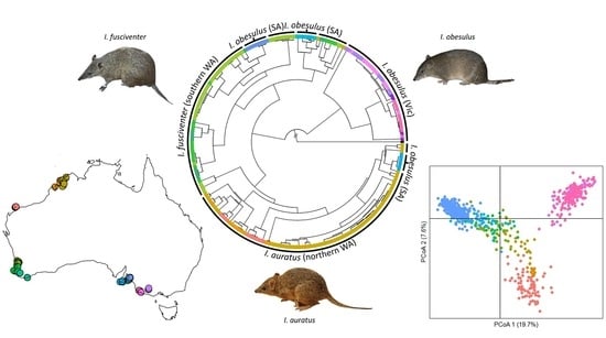
indicates sampling locations. Each pie chart represents haplotype frequencies within each sampling site, and size of pie chart represents numbers of haplotypes. Colour codes indicate the sites where haplotypes were mostly found. Pattern codes represent individual haplotypes found within each site.
Diversity 13 00002 g001
Figure 2. Results of Bayesian phylogenetic analysis in BEAST of D-loop mitochondrial sequences from Isoodon obesulus (Vic, SA), I. fusciventer, and I. auratus. Posterior probability values above 0.9 are indicated by grey circles overlaid on branches. Isoodon macrourus was used as an outgroup. Photo credits: I. auratus Australian Wildlife Conservancy [65], I. fusciventer Dr Kenny Travouillon, Western Australian Museum, I. obesulus Museums Victoria [66].
Diversity 13 00002 g002
Figure 3. Stepwise principal co-ordinates analysis (PCoA) of allele frequencies based on ten microsatellite loci (a,b) and D-loop mtDNA haplotypes (c,d) including (a,c) and excluding (b,d) Victorian I. obesulus samples. Relative PCoA scores have been plotted for the first two dimensions (percentage variation explained on each axis). Individuals are represented in dots, and colours indicate sampling sites.
Diversity 13 00002 g003
Figure 4. Summary of the hierarchical clustering analysis using STRUCTURE based on 10 microsatellite loci. The analyses include (a) all samples, (b) excluding Victoria, (c) excluding Victoria and South Australia, and (d) regional populations. Pie charts on Australia maps illustrate individuals’ estimated membership to each genetic cluster relative to their geographic locations. Barplots in (d) show the most likely K value for each region. Regions include northern Western Australia (NWA), southern Western Australia (SWA), South Australia (SA), and Victoria (VIC). Black lines in barplots separate samples from different sampling locations. Each coloured bar represents an individual with different colours reflecting estimated proportional membership to particular clusters.
Diversity 13 00002 g004
Table 1. Hierarchical AMOVA of mitochondrial DNA performed by grouping sampling sites into regions. Barrow Island (BWI), Kimberley Island (KIMI), Kimberley mainland (KIMM), south west Western Australia (SW WA), Mount Lofty Ranges (MLR), Fleurieu Peninsula (FP), Kangaroo Island (KI), Lower Glenelg (LG).
ComparisonSource of VariationVariance ComponentsPercentagep-Value
BWI, KIMI, KIMMAmong population2.148.3<0.001
Within population2.351.7
Perth metro, SW WA Coast,Among population1.727.9<0.001
SW WA inlandWithin population4.372.1
MLR, FP, KIAmong population5.673.3<0.001
Within population2.026.7
LG, The Grampians, Mount BurrAmong population1.051.6<0.001
Within population1.048.4
Table 2. Pairwise Dest and ϕST values between samples from different locations based on microsatellite (above diagonal) and mtDNA data (below diagonal).
WASAVIC
StateSampling SiteBarrow IslandKimberley IslandsKimberley MainlandPerth MetroSW WA CoastSW WA InlandKangaroo IslandFleurieu PeninsulaMount Lofty RangesThe GrampiansLower GlenelgMount Burr
WABarrow Island0.4360.4780.7010.6820.9020.8170.8170.8680.8620.783
Kimberley islands0.3910.3310.7910.8210.8880.8950.8770.8740.8760.764
Kimberley mainland0.4950.4620.6560.6230.7880.7760.7610.7850.8460.705
Perth metro0.4710.4350.5790.1110.6110.5500.4230.8530.8800.792
SW WA Coast0.5820.5330.6850.318 0.6020.4500.3590.7830.8940.778
SW WA inland0.4370.3890.5640.2620.231
SAKangaroo Island0.8150.7110.7810.5020.6460.5790.5030.5350.8940.9700.899
Fleurieu Peninsula0.5580.4650.660.4240.5650.3750.9220.1830.8700.9710.895
Mount Lofty Ranges0.4000.2840.4450.4150.5200.3830.7540.4040.9130.9600.896
VICGrampians0.8690.8240.8430.7390.8040.7560.9710.9330.8280.3030.302
Lower Glenelg0.8770.8350.8430.7510.8240.7650.9810.9460.8460.7650.177
Mount Burr0.7780.7460.8030.7030.7440.6870.8990.8300.7470.5550.085
Significant Dest values and ϕST values after approximately 1000 permutations are denoted with bold font. Colours represent levels of differentiation from light to dark: 0.0–0.2, 0.2–0.4, 0.4–0.6, 0.6–0.8, and 0.8–1.0.
Table 3. Nuclear and mitochondrial DNA genetic diversity characteristics of Isoodon populations.
StateRegionLocationN
D-loop
NhuhhNHArAFIS
WA 15961610.916 ± 0.0170.023 ± 0.0111720.835 ± 0.03018.1 ± 2.219.0 ± 2.3
North WA8736360.761 ± 0.0510.013 ± 0.0071090.744 ± 0.064 A,C13.1 ± 1.7 A15.0 ± 2.0 A
Barrow Island11770.873 ± 0.0890.010 ± 0.006770.642 ± 0.0843.2 ± 0.38.1 ± 1.30.056
Kimberley Island11880.927 ± 0.0670.015 ± 0.009160.649 ± 0.0513.1 ± 0.27.0 ± 0.90.277
Kimberley mainland6521210.585 ± 0.0750.008 ± 0.005160.861 ± 0.0304.4 ± 0.310.8 ± 1.50.075
South WA7125250.939 ± 0.0140.021 ± 0.011630.786 ± 0.044 A12.0 ± 1.7 A12.1 ± 1.8 A
Perth metro4012100.853 ± 0.0390.018 ± 0.009390.759 ± 0.0513.8 ± 0.39.6 ± 1.00.175
South West Coast13530.782 ± 0.0790.016 ± 0.00970.767 ± 0.0713.8 ± 0.46.0 ± 0.80.231
South West inland1910100.906 ± 0.0410.017 ± 0.009170.787 ± 0.0303.8 ± 0.27.6 ± 0.90.128
SA 21990.857 ± 0.0560.023 ± 0.0123730.623 ± 0.050 B5.7 ± 0.7 B6.9 ± 0.8 B
Mount Lofty Ranges9440.778 ± 0.1100.015 ± 0.0093110.597 ± 0.0522.7 ± 0.25.7 ± 0.80.251
Fleurieu Peninsula4330.833 ± 0.2220.008 ± 0.006450.567 ± 0.0562.6 ± 0.24.4 ± 0.50.458
Kangaroo Island8220.250 ± 0.1800.001 ± 0.001170.422 ± 0.0792.1 ± 0.33.1 ± 0.50.230
VIC 38770.634 ± 0.0600.008 ± 0.0051860.627 ± 0.059 B,C5.8 ± 0.5 B6.7 ± 0.6 B
Grampians11210.182 ± 0.1440.002 ± 0.002270.486 ± 0.0782.3 ± 0.33.1 ± 0.40.243
Lower Glenelg12200.167 ± 0.1340.001 ± 0.001120.444 ± 0.0982.0 ± 0.22.4 ± 0.40.353
Mount Burr11210.327 ± 0.1530.009 ± 0.0051470.612 ± 0.0572.9 ± 0.26.0 ± 0.60.290
mtDNA sample size (ND-loop), number of haplotypes (Nh), number of unique haplotypes (uh), haplotype diversity (h), nucleotide diversity (∏), microsatellite sample size (N), gene diversity (H), allelic richness (Ar), allele number (A), and inbreeding coefficients (FIS). Standard errors are given after mean values. FIS estimates significantly greater than zero after correction for multiple comparisons are denoted with bold font. Statistical differences amongst geographic regions for nuclear diversity parameters were tested using a Friedman’s test and superscripts identify statistically significant groups as determined by post-hoc multiple comparison of group means. Populations with different lettered superscripts are statistically different at p < 0.05.
Publisher’s Note: MDPI stays neutral with regard to jurisdictional claims in published maps and institutional affiliations.

