Density Dependence and Adult Survival Drive Dynamics in Two High Elevation Amphibian Populations


1
Conservation Science Partners, 11050 Pioneer Trail, Suite 202, Truckee, CA 96161, USA
2
National Research Council, Institute of Marine Sciences (CNR-ISMAR), Arsenale, Tesa 104, Castello 2737/F, 30122 Venezia, Italy
3
U.S. Geological Survey, Fort Collins Science Center, 2150 Centre Ave. Bldg C, Fort Collins, CO 80526, USA
*
Author to whom correspondence should be addressed.
Diversity 2020, 12(12), 478; https://doi.org/10.3390/d12120478
Submission received: 30 October 2020
/
Revised: 4 December 2020
/
Accepted: 11 December 2020
/
Published: 15 December 2020
(This article belongs to the Special Issue Biodiversity and Conservation of Tree Frogs)
Abstract
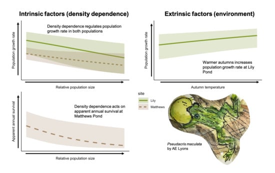
:Amphibian conservation has progressed from the identification of declines to mitigation, but efforts are hampered by the lack of nuanced information about the effects of environmental characteristics and stressors on mechanistic processes of population regulation. Challenges include a paucity of long-term data and scant information about the relative roles of extrinsic (e.g., weather) and intrinsic (e.g., density dependence) factors. We used a Bayesian formulation of an open population capture-recapture model and >30 years of data to examine intrinsic and extrinsic factors regulating two adult boreal chorus frogs (Pseudacris maculata) populations. We modelled population growth rate and apparent survival directly, assessed their temporal variability, and derived estimates of recruitment. Populations were relatively stable (geometric mean population growth rate >1) and regulated by negative density dependence (i.e., higher population sizes reduced population growth rate). In the smaller population, density dependence also acted on adult survival. In the larger population, higher population growth was associated with warmer autumns. Survival estimates ranged from 0.30–0.87, per-capita recruitment was <1 in most years, and mean seniority probability was >0.50, suggesting adult survival is more important to population growth than recruitment. Our analysis indicates density dependence is a primary driver of population dynamics for P. maculata adults.
1. Introduction
Progress in mitigating declines in animal populations depends on moving beyond the identification of causes and towards the determination of mechanism—how a particular cause affects whole populations. A prerequisite for making sense of such mechanisms is to understand how populations are regulated (e.g., intrinsically or extrinsically) and then to understand how regulation is affected by cause(s) of decline (e.g., a system perturbed by disease or invasive species). The past three decades of amphibian declines illustrate a progression in conservation efforts from identifying a phenomenon [1], to identifying potential causes [2,3,4], to searching for mechanisms [5,6] and identifying mitigation strategies [7,8,9]. However, the prerequisite to assembling these pieces of information is an understanding of how amphibian populations are regulated, and this is incomplete [10,11]. Regulation is likely a combination of the effects of intrinsic (e.g., density dependence, [12,13]) and extrinsic (e.g., environmental [14,15]) factors and their interactions.
Much of the current work on amphibian populations focuses on the effects of various environmental (extrinsic) factors on individual demographic parameters such as survival, recruitment, or population growth rate [15,16,17,18,19,20,21,22,23,24]. There is less work examining the effect of intrinsic factors (i.e., density dependence) on population regulation, especially for terrestrial life stages. There are notable exceptions that examine the role of density dependence in amphibian populations [25,26,27,28,29], and Leão et al. [13] provide broad evidence for density dependent population regulation in amphibians and reptiles, including three species of Pseudacris. However, the majority of these studies rely on count data that do not account for observation error (but see [29]), and thus, are more likely to detect spurious effects of density dependence [30,31].
Density dependence can act on different life stages (e.g., embryonic, larval, terrestrial), but also on different demographic rates (e.g., fecundity, recruitment, survival)—such influences can be problematic for amphibians, in particular those that have complex life histories that involve metamorphosis and the use of different habitats [10]. Determining at what stage(s) density dependence matters, and which rate(s) it affects, is a key component in understanding population regulation and mechanisms behind observed declines.
Exploring factors that regulate populations requires data series that encompass population information over a long enough time period to record decreases and increases (i.e., due to perturbations and recoveries) in population size. Long-term data sets can meet this requirement and increase confidence in the effect of a given factor (whether intrinsic or extrinsic) on a demographic rate [32,33,34]. Long-term data sets typically avoid pitfalls common to analyses of short-term data (e.g., shifting baselines [35,36], erroneous identification of population trends [37], inconclusive relationships among demographic parameters of interest and covariates [4], or opposing results [38]).
Relative to the number of amphibian species with conservation concerns, there are few amphibian studies with data amenable to testing the effect of density dependence on demographic rates (e.g., capture-mark-recapture or similar). This limitation makes extant data sets particularly valuable [31]. Furthermore, many of these studies were initiated because of identified threats to populations of interest, suggesting that these populations (and factors that regulate them) were responding to, or recovering from, perturbation. Populations responding to such circumstances likely do not provide representative data from which to build hypotheses about how amphibian populations are regulated [35,36,37].
In addition to understanding the factors that regulate a population, it is also important to know the demographic structure of a population. For example, knowing the relative contribution of new recruits versus surviving individuals to the overall population growth rate provides a bridge between understanding the mechanisms that regulate a population and the management of that population [11]. If a population is relatively stable and survival is estimated to be low and recruitment high, this may indicate that the growth rate is more sensitive to changes in new recruits, giving managers insight into which demographic parameter to target if population growth rate declines. Thus, ideal models provide (1) estimates of the effects of intrinsic vs. extrinsic factors on one or more demographic parameters that regulate population growth, and (2) a robust assessment of the demographic composition of a population.
In contrast to threatened and endangered amphibians, the boreal chorus frog (Psuedacris maculata) is a species of least concern (ICUN https://www.iucnredlist.org/species/136004/78906835) and is common in Colorado [39]. We have been studying boreal chorus frogs at two sites in northern Colorado since the 1960s, using continuously collected capture-mark-recapture (cmr) methods since the mid-1980s. To effectively use these data (35 yrs and ~11 generations [40]), we employed a recent extension of the temporal symmetry model, also known as the Pradel model [41,42], to (1) estimate the effects of density dependence and environment (e.g., temperature, snowpack, drought) on demographic parameters and population growth rates of adult boreal chorus frogs, and (2) provide robust estimates of realized population growth rate, apparent survival, and recruitment over the course of the time series.
2. Materials and Methods
2.1. Species
Boreal chorus frogs are members of the acrisinae subfamily within the family Hylidae. The genus Pseudacris (trilling chorus frogs, sensu Moriarty-Lemmon et al. 2007) is endemic to North America and occurs throughout much of the U.S. [43,44]. The mean snout-vent-length for boreal chorus frogs at our sites is 32.44 mm (Corn and Muths unpublished data), and there is evidence that individuals from high-elevation populations are smaller than individuals at lower elevations [45,46]. Boreal chorus frogs mature at 2–3 years [47] and cmr data suggest that the average life span is 5–7 years with some individuals living >10 years (Muths, unpublished data). After an explosive breeding season triggered by snowmelt [48], adults are primarily terrestrial (e.g., inhabiting wet meadows). Unlike other hylids adapted to arboreal habitats, the eyes of boreal chorus frogs do not face forward and they lack adhesive pads on their toes. Genetic connectivity in boreal chorus frogs is associated with landscape complexity (i.e., topography, differences in moisture), and migration/colonization is facilitated by stepping-stone habitats [49].
2.2. Data Collection
Capture-mark-recapture data were collected in a robust-design framework [50] for two populations of chorus frogs that breed in ephemeral, subalpine ponds in northern Colorado from 1986 through 2020 (Figure 1). Briefly, frogs were captured by hand on multiple occasions during the breeding season each year at each pond [51]. From 1986–2010, frogs were marked by toe clipping and from 2010 onwards, with visual implant elastomer and toe clipping. Lily Pond (LP, elevation = 2969 m) and Matthews Pond (MP, elevation = 2803 m) are approximately 3.6 km apart, embedded in a forest of lodgepole pine (Pinus contorta), Engelmann spruce (Picea engelmannii), and subalpine fir (Abies lasiocarpa). Lily Pond is larger than MP (0.66 ha and 0.20 ha, respectively), such that the canopy at MP is more closed. Pond vegetation includes grasses (Poacea), sedges (Cyperaceae), cattails (Typhaceae), and water lilies (Nymphaeaceae). Ponds fill as snow melts and dry completely by late August. The data collection was done through USGS under the following animal care number: FORT IACUC 2013-09_RENEWAL_B, Issued May 2019.
2.3. Covariate Development
We derived a suite of extrinsic weather covariates (Table 1) and a density dependent (intrinsic) covariate to test in our modeling framework. Weather covariates (representative of current climate conditions) were hypothesized to affect survival and recruitment of P. maculata and were based on a subset of covariates developed by Muths et al. [51]. We used temperature and snowpack data from the nearest SNOTEL station (Joe Wright, <6 km from study sites, elevation = 3085 m) for most years, and data from Grizzly Peak, 110 km from study sites, elevation = 3383 m, when data were unavailable from Joe Wright (1986–1989). Comparisons among site-specific temperatures and data from SNOTEL sites showed high correspondence [51]. We used the package ‘snotelr’ [52] in the statistical programing language R [53] to download SNOTEL data and derive covariates for modeling. The summer drought covariate was derived from the Palmer Hydrological Drought Index for Colorado (https://www7.ncdc.noaa.gov/CDO/CDODivisionalSelect.jsp#, accessed 7 August 2020). We did not include covariates in the model that were highly correlated (i.e., Pearson’s correlation coefficient >0.70). For all extrinsic covariates, we used data summarized over the year for which we estimated survival (e.g., for survival from 1986–1987, we calculated the coldest average seven days in the winter between 1 October 1986 and 1 March 1987).
To test the effect of density dependence, we derived an index of population size (), where Ni is abundance at time (year) i (with i = 1, …, 35). Abundance was derived from cmr data for each time step in the Pradel model as a function of the number of individuals that survived from time i to i + 1 and the number of recruits added to the population in each time step [42]. We used the abundance relative to abundance at i = 2 because there are known issues with estimating abundance in the first time step for time-dependent Jolly-Seber models (of which the Pradel model is a class) and relative abundance is less sensitive to capture heterogeneity [42].
2.4. Data Analysis
We modified the Bayesian formulation of the Pradel model developed by Tenan et al. [42] to estimate realized population growth rate (ρ), annual apparent survival probability (φ), annual detection probability (p), seniority probability (γ), and per-capita recruitment for both populations. Among the different approaches that exist to estimate and model population growth and associated vital rates using cmr data from open populations, the Pradel model has the unique characteristic of combining the standard-time and the reverse-time approach of reading individual longitudinal data in the same likelihood, simultaneously incorporating survival and recruitment parameters, and thus allowing inference on population growth rate. The conceptual basis of the Pradel model derives from the observation that the proportion of individuals that are already members of the population in the previous sampling occasion is the analogue of the survival rate when capture histories are considered in reverse time order. Pradel [41] posited that the proportion of the seniority parameter (γ) reflects the relative contribution of survivors from the previous occasion to the population growth rate. The model formulation used here incorporates an index of population size and represents a model-based approach to formally test and quantify the strength of density dependence directly on population growth rate, as well as related vital rates, from cmr data. We used a parametrization of model likelihood where ρ, φ, and p were model parameters estimated directly, and γ and per-capita recruitment were derived parameters. Specifically, seniority probability γi represents the probability that an individual is in the population at time i, given it was in the population at time i-1, and was derived as φi−1/ρi−1. Per-capita recruitment (i.e., the number of individuals entering the population at time i, via local recruitment or immigration, per individual already in the population) was derived as ρi−φi [42]. Thus, we tested the effects of density dependence and weather covariates on population growth rate ρ using the following linear predictor, which included a random effect of year (i):
where
and where Pi = Ni/N2 (e.g., the population size relative to population size at year i = 2) is the density dependent term. We used the following equation to estimate survival probability (φ):
where
Finally, we modeled detection probability as a random effect that varied by year.
We implemented the model in JAGS through the R package ‘jagsUI’ [54]. We ran three chains with 3,150,000 iterations each, including an adapt phase of 50,000 iterations and a burn in of 100,000 iterations. We thinned each chain to every 300 iterations; thus, our final posterior distribution consisted of 30,000 iterations. We assessed model convergence using the R-hat statistic [55,56], which was <1.1 for all parameters. We considered a covariate to have a significant effect if the 95% credible interval (95% CRI) did not overlap zero. Finally, we calculated the geometric mean growth rate for each population [57,58] to assess whether the two populations were, on average, growing, declining, or stable over the course of the 34-year time series (see Tenan et al. [42], the supplementary code, for details on prior parameter distributions and model formulation).
3. Results
We used capture histories for 2490 unique male frogs and 200 unique female frogs at LP, and 1125 unique male frogs and 108 unique female frogs at MP in our models. The difference in the number of males and females is a result of a reduced catchability of females, and thus, our estimates of population growth rate and demographic rates are driven largely by males. Mean detection probability at LP was 0.16 (95% credible interval [CRI], 0.14–0.19) and 0.25 (CRI 0.20–0.32) at MP.
3.1. Population Growth Rate
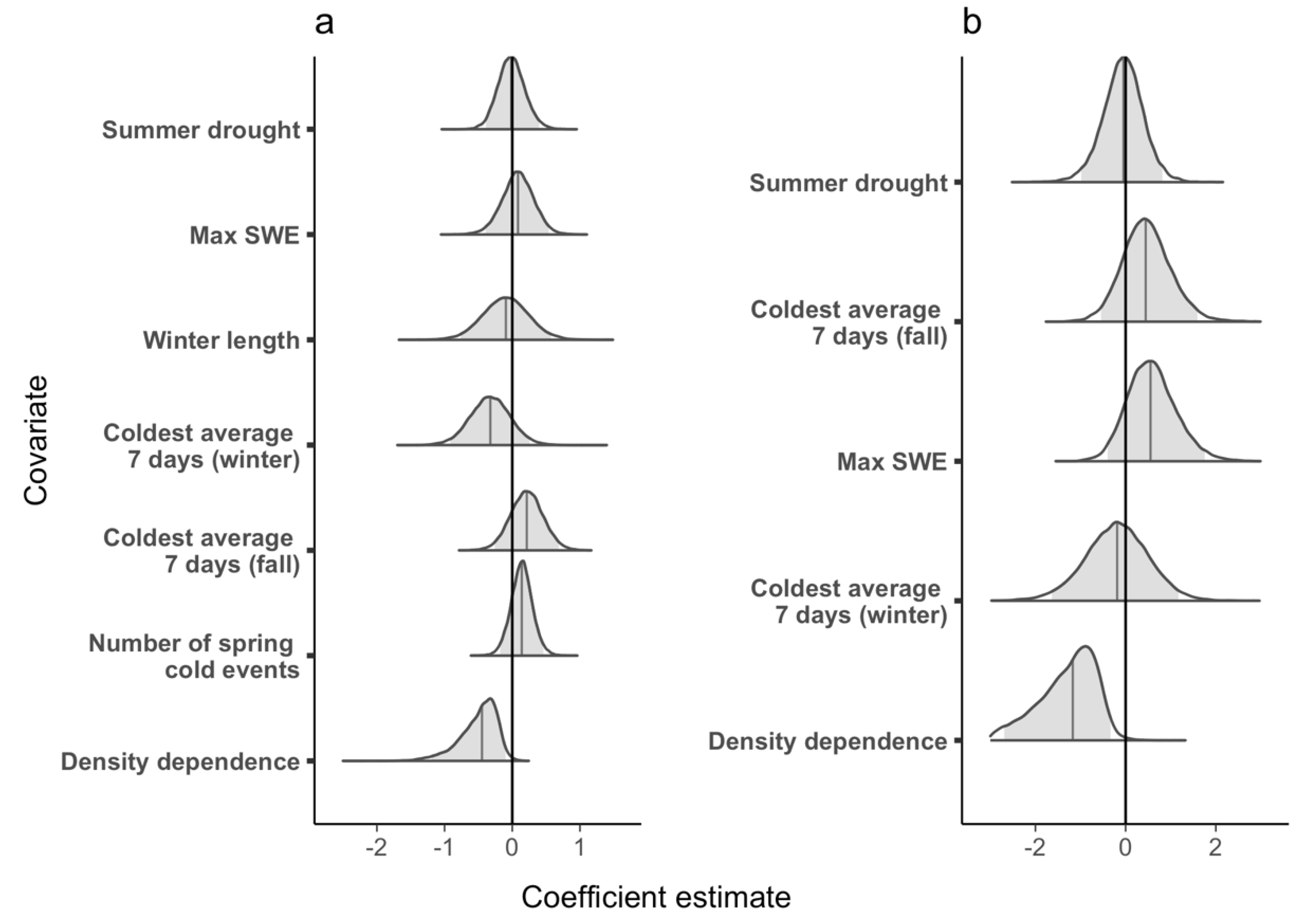
The geometric mean realized population growth rate for LP was 1.07 (CRI 0.62–1.71), suggesting a population that grew, on average, by 7% per year. Population growth rate (ρ) was highest in 1987 (2.68, CRI 1.00–5.44) and lowest in 2014 (0.51, CRI 0.28–0.83), and in 21 of the 34 years at LP, the population growth rate was >1.00 (Figure 2a). Higher relative population size at LP had a significantly negative effect on population growth rate (Figure 3a) and the proportion of temporal variance explained was 0.48, suggesting that negative density dependence is regulating the population. Of the weather covariates, only the minimum average 7-day temperature in autumn (tmin7fl) had a significant effect on population growth rate (i.e., warmer autumns had a significantly positive effect on population growth rate, Figure 3a), but the proportion of temporal deviance explained was small (0.007).
The geometric mean realized population growth rate for MP was 1.06 (CRI 0.55–1.84) and ranged from 0.60 (CRI 0.24–1.13) in 1990 to 1.88 (CRI 0.88–3.70) in 1995. The population growth rate was >1.00 in 18 of 34 years (Figure 4a). The density dependence covariate had a significant effect on the population growth rate at MP and the proportion of temporal variance explained was 0.28, but no weather covariates had a significant effect (Figure 5a). As with LP, the effect was negative, suggesting that higher population size results in lower population growth rate.
3.2. Survival
The apparent survival probability (φ) at LP ranged from 0.18 (CRI 0.03–0.48) in 1987 to 0.87 (CRI 0.70–0.98) in 2005, and mean survival probability (i.e., the inverse-logit of the intercept) was 0.49 (CRI 0.15–0.80). In general, survival probability increased from 1987–2008, decreased from 2009–2018, then increased again in 2019 and 2020 (Figure 2b). Neither the weather covariates that we tested nor the density dependence term affected survival at LP (i.e., 95% credible intervals of the coefficient estimates overlapped zero in all cases, Figure 3b). Apparent survival probability at MP ranged from 0.30 (95% CRI 0.08–0.62) in 1990 to 0.78 (CRI 0.45–0.99) in 2011 (Figure 4b), and the mean was 0.42 (CRI 0.34–0.69). Density dependence had a negative effect on survival probability at MP and the temporal variance explained was 0.65, suggesting that density dependence is regulating apparent survival at the adult stage (e.g., survival decreases or permanent emigration increases as population sizes increase, Figure 5b). No weather covariates had a significant effect on survival probability at MP (Figure 5b).
3.3. Additional Parameters
We observed substantial variation in seniority probability (γ) at LP over time, ranging from 0.08 (CRI 0.01–0.23) in 1988 to 1.00 in 1987 and 2004 (CRI 0.34–1.00 and 0.89–1.0, respectively) (Figure 2c). However, the mean γ for LP was 0.61 (CRI 0.38–0.83), suggesting that adults that are already in the population contribute disproportionately to population growth rate (i.e., over half of the individuals in the population are surviving adults). Seniority probability was also variable at MP, ranging from 0.30 (CRI 0.17–0.46) in 2013 to 0.88 (95% CRI 0.55–1.00) in 2008 (Figure 4c). Although lower than at LP, mean seniority probability at MP (0.54, CRI 0.31–0.82) was also >0.50, suggesting a disproportionate effect of survivors on population growth rate similar to LP. Per-capita recruitment at LP was <1.00 in 30 of 34 years, and ranged from 0 in 2003 to 2.5 in 1987 (CRI 0.97–4.96) (Figure 2d). Similarly, per-capita recruitment at MP was <1.00 in 30 of 34 years, and ranged from 0.13 (CRI 0–0.40) in 2007 to 1.14 (CRI 0.49–2.82) in 1995 (Figure 4d).
4. Discussion
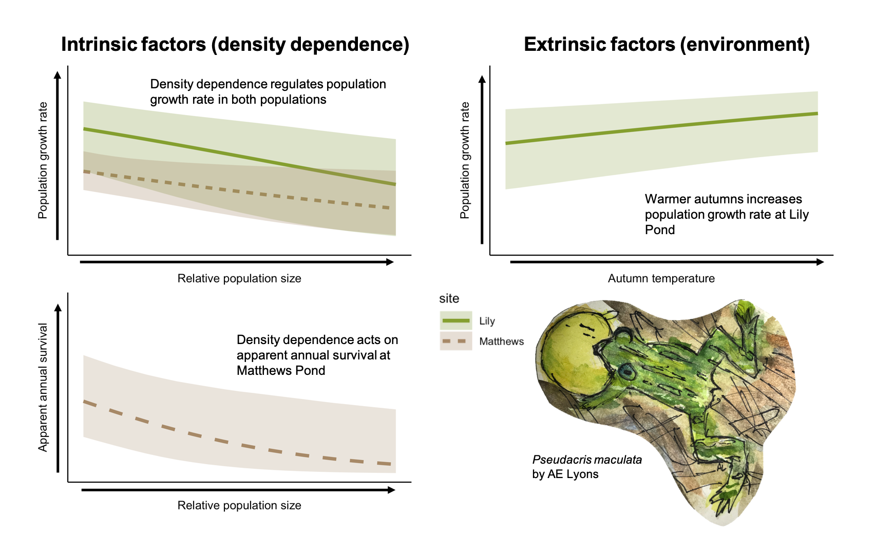
Responding to declining populations requires foundational knowledge of the mechanisms of population regulation prior to declines. We explored the relative contribution of intrinsic and extrinsic factors regulating two populations of P. maculata using data from two relatively stable populations (i.e., no evidence of dramatic declines in >50 years of data collection). We identified negative density dependence as the primary driver of population growth rates for both populations. For the smaller of the two populations (MP), there was a negative effect of density on apparent adult survival. This suggests that when relative abundance is high, population growth rate declines (and conversely, when relative abundance is low, growth rate increases), resulting in stable oscillation around a realized population growth rate of one. While there was some evidence that warmer autumns result in increased population growth rate for LP (the larger population), the proportion of temporal deviance explained in population growth rate was small (0.007), and the proportion of temporal deviance explained by the density dependence term was relatively large (0.48). With the exception of warmer autumns at LP, no other weather covariates that we tested had an effect on growth rate or survival, suggesting that intrinsic density dependence primarily regulates demographic patterns in these populations.
The Bayesian hierarchical formulation of the Pradel model provided robust estimates of population growth rate and demographic parameters (apparent survival, seniority probability, and per-capita recruitment) for all years, including those not estimable in a previous analysis [51]. In that analysis, a classical formulation of the Pradel model fitted in a frequentist framework was used to directly estimate apparent survival, recruitment, and population growth rate at LP and MP, but these parameters were not estimable for one-third of the years in each of the time series, likely because there were fewer captures and recaptures in those years. A Bayesian formulation of the Pradel model permits the hierarchical modeling of the biological and sampling processes and allows the extension of the original fixed time effects structure to random time effects, an option that is still impractical in a frequentist framework and can help address issues of convergence [59]. By including a random effect of year, for years with small sample sizes, information is pooled from years with larger sample sizes [56].
Our observed patterns of population growth rate and parameter estimates aligned with earlier results [51]. Specifically, periods of increases and decreases in growth rate were consistent, and mean estimates of survival were nearly identical: LP = 0.50, MP = 0.43 [51], and LP = 0.49, MP = 0.42 (present study); capture probabilities were also comparable: LP = 0.005−0.496, MP = 0.008−0.778 [51], and LP = 0.102−0.38, MP = 0.134−0.46 (present study). The smaller range in capture probabilities in our current analysis may be due to the random temporal structure we used, which ‘shrinks’ estimates towards the population mean [54].
Importantly, however, average population growth rates between the two analyses were different. Our analysis indicates that mean population growth rates were similar for LP (1.07) and MP (1.06), whereas Muths et al. [51] reported mean population growth rates of 1.14 for LP and 0.88 for MP, suggesting a declining population at MP. Despite a 29-year data set, the earlier growth rates were estimable for only 20 (LP) and 19 (MP) years. Because we used a Bayesian framework, we were able to estimate growth rate for the full time series available (i.e., 29 years from the previous analysis plus an additional five years of data), and thus, we consider our results to be more robust.
The complementary results from the two analyses provide, at minimum, hypotheses to test further. For instance, our analysis provides some evidence that warmer autumns (as an analog to longer summers) may influence population growth rate of adults at LP, while the previous work [51] indicates that drought and longer summers have a negative effect on recruitment. Understanding whether increased survival at the adult stage compensates for reduced recruitment under future climate conditions (summers are expected to be longer) is key for teasing apart the effects of climate change on overall population stability [24,60]. The discrepancy in average growth rates between the two analyses highlights the importance of complete data series for estimating population trends [32] and the utility of re-examining long time series of data as new analytical approaches become available that can address issues related to small sample sizes (e.g., few recaptures). For example, although the data used in the earlier analysis were complete from a field standpoint (i.e., data were collected in every year of the time series), some parameters were not estimable using the Pradel model in a frequentist framework.
Estimates of population growth rate are important for identifying trends in the relative abundance of a population, and estimates of survival provide context for observed patterns in population growth rate. To improve our contextual understanding of these populations, we derived estimates for two additional demographic parameters that are important for understanding underlying population dynamics: seniority probability (i.e., the probability that an individual in the population at time i was also in the population at time i-1 [41]) and per-capita recruitment. We found that for both populations, mean seniority probability was high (> 0.50), while per-capita recruitment was low (generally, <1 individual recruited to the population for every individual already in the population). This suggests that for P. maculata, adults that are already in the population are critical for maintaining population stability, and that the population growth rate is likely more sensitive to changes in adult survival than changes in recruitment, a result that supports our supposition above, relative to the importance of warmer autumns. The idea that adult life stages contribute disproportionately to population growth rate in amphibians has been demonstrated with matrix projection models based on asymptotic growth rates [11,24,61,62], but empirical data that confirm this (e.g., data that can be used to quantify realized population growth rates) are rare. This is particularly true for small Hylids that tend to have low capture rates due to large population sizes and logistical constraints (e.g., additional survey effort needed to find small individuals). Our analysis thus provides novel insight into Hylid population dynamics, information that can be used to guide management decisions (e.g., determining which life stage to target in conservation actions), but that was previously inconclusive in prior analyses [51].
Understanding the intrinsic and extrinsic factors regulating each life stage is also important for managing under environmental uncertainty (e.g., threat of climate change, disease). We identified only one extrinsic factor that potentially affected estimates of population growth rate (warmer autumns), but our study focused solely on adults. Other life stages (embryos, larvae, juveniles) may be more sensitive to extrinsic factors. For example, temperatures are expected to increase and snowpack decrease for many montane environments [63], resulting in reduced hydroperiod length and the potential for increased larval mortality [24,64,65,66]. Previous work indicates that plasticity in P. maculata larvae is limited and suggests that larval survival and somatic growth are linked to historical (rather than current) hydroperiod conditions [64]. Thus, given climate predictions, it is reasonable to hypothesize that larval mortality could reach levels that affect population growth rates despite evidence that adult survival is the main driver [24].
These results are likely useful in understanding demographic responses to causes of decline in other similar species and provide a solid baseline for this species should it become threatened in the future. For example, while we demonstrate that population growth rate and survival are largely invariant to weather patterns, our analysis does not address emerging infectious disease [67] or the indirect effects of climate change, such as increased incidence and intensity of wildfire [68,69]. Both LP and MP were recently affected by the 2020 Cameron Peak wildfire, the largest wildfire in Colorado history (https://www.denverpost.com/2020/10/18/cameron-peak-fire-update-october-18/). More broadly, over 3-million hectares have burned in Oregon, California, and Washington in 2020, putting multiple species at risk [69]. Fires in Australia in 2019 were similarly unprecedented [70]. Most studies of amphibian response to wildfire have focused on community composition and occupancy pre and post-wildfire (toads [71], frogs and salamanders [72]), but there is also evidence that fire reduces effective population size and increases extinction risk for tree frogs (Litoria spp [73]). The threat of the Cameron Peak fire underscores the value of the long-term data collection efforts at LP and MP. The intensive study design allows for a robust comparison of ‘baseline’ conditions to data gathered in post-fire years contributing to a better understanding of the demographic response of amphibian populations to fire.
We have improved demographic estimates for our target populations and enlarged our context for thinking about population dynamics in a small Hylid amphibian species that is currently widespread in North America and non-threatened. These long-term data collected from a species that has not experienced catastrophic declines, and from populations that have not been significantly affected by anthropogenic activities, provide robust estimates of demographic parameters and insight into the factors regulating these populations. This contribution will be useful to managers requiring estimates that are reliable and that can be used with confidence in viability modeling or in determining the consequences of management actions, particularly for species that cannot be reliably and directly censused. Such information will also contribute to our understanding of population regulation in amphibians, which has relevance to population theory as well as conservation.
Author Contributions
Conceptualization, A.M.K. and E.M.; Data collection: E.M., Methodology, A.M.K., S.T. and E.M.; Software, S.T.; Formal Analysis, A.M.K. and S.T.; Resources, E.M.; Data Curation, E.M. and A.M.K.; Writing, A.M.K. and E.M. All authors have read and agreed to the published version of the manuscript.
Funding
This research received no external funding.
Acknowledgments
We thank B. Dickson for a helpful review of the manuscript. Any use of trade, firm, or product names is for descriptive purposes only and does not imply endorsement by the U.S. Government. This is contribution number 774 of the U.S. Geological Survey Amphibian Research and Monitoring Initiative (ARMI).
Conflicts of Interest
The authors declare no conflict of interest.
References
- Blaustein, A.R.; Wake, D.B. Declining amphibian populations: A global phenomenon? Trends Ecol. Evol. 1990, 5, 203–204. [Google Scholar] [CrossRef]
- Daszak, P.; Scott, D.E.; Kilpatrick, A.M.; Faggioni, C.; Gibbons, J.W.; Porter, D. Amphibian population declines at Savannah river site are linked to climate, not Chytridiomycosis. Ecology 2005, 86, 3232–3237. [Google Scholar] [CrossRef]
- Knapp, R.A.; Boiano, D.M.; Vredenburg, V.T. Removal of nonnative fish results in population expansion of a declining amphibian (mountain yellow-legged frog, Rana muscosa). Biol. Conserv. 2007, 135, 11–20. [Google Scholar] [CrossRef] [PubMed] [Green Version]
- Grant, E.H.C.; Miller, D.A.W.; Schmidt, B.R.; Adams, M.J.; Amburgey, S.M.; Chambert, T.; Cruickshank, S.S.; Fisher, R.N.; Green, D.M.; Hossack, B.R.; et al. Quantitative evidence for the effects of multiple drivers on continental-scale amphibian declines. Sci. Rep. 2016, 6, 25625. [Google Scholar] [CrossRef] [PubMed] [Green Version]
- Skelly, D.K. Distributions of pond-breeding anurans: An overview of mechanisms. Isr. J. Zool. 2001, 47, 313–332. [Google Scholar] [CrossRef]
- Longo, A.V.; Burrowes, P.A.; Joglar, R.L. Seasonality of Batrachochytrium dendrobatidis infection in direct-developing frogs suggests a mechanism for persistence. Dis. Aquat. Org. 2010, 92, 253–260. [Google Scholar] [CrossRef]
- Garner, T.W.J.; Rowcliffe, J.M.; Fisher, M.C. Climate change, chytridiomycosis or condition: An experimental test of amphibian survival. Glob. Chang. Biol. 2011, 17, 667–675. [Google Scholar] [CrossRef]
- Canessa, S.; Bozzuto, C.; Grant, E.H.C.; Cruickshank, S.S.; Fisher, M.C.; Koella, J.C.; Lötters, S.; Martel, A.; Pasmans, F.; Scheele, B.C.; et al. Decision-making for mitigating wildlife diseases: From theory to practice for an emerging fungal pathogen of amphibians. J. Appl. Ecol. 2018, 55, 1987–1996. [Google Scholar] [CrossRef] [Green Version]
- Petrovan, S.O.; Schmidt, B.R. Neglected juveniles; a call for integrating all amphibian life stages in assessments of mitigation success (and how to do it). Biol. Conserv. 2019, 236, 252–260. [Google Scholar] [CrossRef]
- Hellriegel, B. Single- or multistage regulation in complex life cycles: Does it make a difference? Oikos 2000, 88, 239–249. [Google Scholar] [CrossRef]
- Biek, R.; Funk, W.C.; Maxell, B.A.; Mills, L.S. What is missing in amphibian decline research: Insights from ecological sensitivity analysis. Conserv. Biol. 2002, 16, 728–734. [Google Scholar] [CrossRef]
- Beverton, R.J.H.; Holt, S.J. On the Dynamics of Exploited Fish Populations; Springer Science & Business Media: Berlin/Heidelberg, Germany, 2012; ISBN 978-94-011-2106-4. [Google Scholar]
- Leão, S.M.; Pianka, E.R.; Pelegrin, N. Is there evidence for population regulation in amphibians and reptiles? J. Herpetol. 2018, 52, 28–33. [Google Scholar] [CrossRef]
- Briggs, C.J.; Vredenburg, V.T.; Knapp, R.A.; Rachowicz, L.J. Investigating the population-level effects of chytridiomycosis: An emerging infectious disease of amphibians. Ecology 2005, 86, 3149–3159. [Google Scholar] [CrossRef]
- Reading, C.J. Linking global warming to amphibian declines through its effects on female body condition and survivorship. Oecologia 2007, 151, 125–131. [Google Scholar] [CrossRef]
- Bell, B.D.; Carver, S.; Mitchell, N.J.; Pledger, S. The recent decline of a New Zealand endemic: How and why did populations of Archey’s frog Leiopelma archeyi crash over 1996–2001? Biol. Conserv. 2004, 120, 189–199. [Google Scholar] [CrossRef]
- Schmidt, B.R.; Feldmann, R.; Schaub, M. Demographic processes underlying population growth and decline in Salamandra salamandra. Conserv. Biol. 2005, 19, 1149–1156. [Google Scholar] [CrossRef]
- Bell, B.D.; Pledger, S.A. How has the remnant population of the threatened frog Leiopelma pakeka (Anura: Leiopelmatidae) fared on Maud Island, New Zealand, over the past 25 years? Austral Ecol. 2010, 35, 241–256. [Google Scholar] [CrossRef]
- McCaffery, R.M.; Maxell, B.A. Decreased winter severity increases viability of a montane frog population. Proc. Natl. Acad. Sci. USA 2010, 107, 8644–8649. [Google Scholar] [CrossRef] [Green Version]
- Muths, E.; Scherer, R.D.; Pilliod, D.S. Compensatory effects of recruitment and survival when amphibian populations are perturbed by disease. J. Appl. Ecol. 2011, 48, 873–879. [Google Scholar] [CrossRef]
- Muths, E.; Chambert, T.; Schmidt, B.R.; Miller, D.a.W.; Hossack, B.R.; Joly, P.; Grolet, O.; Green, D.M.; Pilliod, D.S.; Cheylan, M.; et al. Heterogeneous responses of temperate-zone amphibian populations to climate change complicates conservation planning. Sci. Rep. 2017, 7, 17102. [Google Scholar] [CrossRef] [Green Version]
- Hossack, B.R.; Adams, M.J.; Pearl, C.A.; Wilson, K.W.; Bull, E.L.; Lohr, K.; Patla, D.; Pilliod, D.S.; Jones, J.M.; Wheeler, K.K.; et al. Roles of patch characteristics, drought frequency, and restoration in long-term trends of a widespread amphibian. Conserv. Biol. 2013, 27, 1410–1420. [Google Scholar] [CrossRef] [PubMed]
- Cayuela, H.; Arsovski, D.; Thirion, J.-M.; Bonnaire, E.; Pichenot, J.; Boitaud, S.; Brison, A.-L.; Miaud, C.; Joly, P.; Besnard, A. Contrasting patterns of environmental fluctuation contribute to divergent life histories among amphibian populations. Ecology 2016, 97, 980–991. [Google Scholar] [CrossRef] [PubMed]
- Kissel, A.M.; Palen, W.J.; Ryan, M.E.; Adams, M.J. Compounding effects of climate change reduce population viability of a montane amphibian. Ecol. Appl. 2019, 29, e01832. [Google Scholar] [CrossRef] [PubMed]
- Beebee, T.J.C.; Denton, J.S.; Buckley, J. Factors affecting population densities of adult Natterjack toads Bufo calamita in Britain. J. Appl. Ecol. 1996, 33, 263–268. [Google Scholar] [CrossRef]
- Meyer, A.H.; Schmidt, B.R.; Grossenbacher, K. Analysis of three amphibian populations with quarter–century long time–series. Proc. R. Soc. Lond. Ser. B Biol. Sci. 1998, 265, 523–528. [Google Scholar] [CrossRef]
- Pellet, J.; Schmidt, B.R.; Fivaz, F.; Perrin, N.; Grossenbacher, K. Density, climate and varying return points: An analysis of long-term population fluctuations in the threatened European tree frog. Oecologia 2006, 149, 65–71. [Google Scholar] [CrossRef]
- Băncilă, R.I.; Ozgul, A.; Hartel, T.; Sos, T.; Schmidt, B.R. Direct negative density-dependence in a pond-breeding frog population. Ecography 2016, 39, 449–455. [Google Scholar] [CrossRef]
- Cayuela, H.; Griffiths, R.A.; Zakaria, N.; Arntzen, J.W.; Priol, P.; Léna, J.-P.; Besnard, A.; Joly, P. Drivers of amphibian population dynamics and asynchrony at local and regional scales. J. Anim. Ecol. 2020, 89, 1350–1364. [Google Scholar] [CrossRef]
- Freckleton, R.P.; Watkinson, A.R.; Green, R.E.; Sutherland, W.J. Census error and the detection of density dependence. J. Anim. Ecol. 2006, 75, 837–851. [Google Scholar] [CrossRef] [Green Version]
- Lebreton, J.-D. Assessing density dependence: Where are we left? In Modeling Demographic Processes in Marked Populations; Thomson, D.L., Cooch, E.G., Conroy, M.J., Eds.; Springer Science & Business Media: Berlin/Heidelberg, Germany, 2009; ISBN 978-0-387-78151-8. [Google Scholar]
- Pechmann, J.H.K.; Scott, D.E.; Semlitsch, R.D.; Caldwell, J.P.; Vitt, L.J.; Gibbons, J.W. Declining amphibian populations: The problem of separating human impacts from natural fluctuations. Science 1991, 253, 892–895. [Google Scholar] [CrossRef] [Green Version]
- Lindenmayer, D.B.; Likens, G.E.; Andersen, A.; Bowman, D.; Bull, C.M.; Burns, E.; Dickman, C.R.; Hoffmann, A.A.; Keith, D.A.; Liddell, M.J.; et al. Value of long-term ecological studies. Austral Ecol. 2012, 37, 745–757. [Google Scholar] [CrossRef]
- Hughes, B.B.; Beas-Luna, R.; Barner, A.K.; Brewitt, K.; Brumbaugh, D.R.; Cerny-Chipman, E.B.; Close, S.L.; Coblentz, K.E.; de Nesnera, K.L.; Drobnitch, S.T.; et al. Long-term studies contribute disproportionately to ecology and policy. BioScience 2017, 67, 271–281. [Google Scholar] [CrossRef] [Green Version]
- Pauly, D. Anecdotes and the shifting baseline syndrome of fisheries. Trends Ecol. Evol. 1995, 10, 430. [Google Scholar] [CrossRef]
- Dayton, P.K.; Tegner, M.J.; Edwards, P.B.; Riser, K.L. Sliding baselines, ghosts, and reduced expectations in kelp forest communities. Ecol. Appl. 1998, 8, 309–322. [Google Scholar] [CrossRef]
- Pechmann, J.H.K.; Wilbur, H.M. Putting declining amphibian populations in perspective: Natural fluctuations and human impacts. Herpetologica 1994, 50, 65–84. [Google Scholar]
- Lindenmayer, D.B.; Cunningham, R.B. Longitudinal patterns in bird reporting rates in a threatened ecosystem: Is change regionally consistent? Biol. Conserv. 2011, 144, 430–440. [Google Scholar] [CrossRef]
- Hammerson, G.A. Amphibians and Reptiles in Colorado, Revised Edition, 2nd ed.; University Press of Colorado: Niwot, CO, USA, 1999; ISBN 978-0-87081-534-8. [Google Scholar]
- Ricklefs, R.E. The Economy of Nature by Ricklefs, 5th ed.; W. H. Freeman: New York, NY, USA, 2001. [Google Scholar]
- Pradel, R. Utilization of capture-mark-recapture for the study of recruitment and Population growth rate. Biometrics 1996, 52, 703–709. [Google Scholar] [CrossRef]
- Tenan, S.; Tavecchia, G.; Oro, D.; Pradel, R. Assessing the effect of density on population growth when modeling individual encounter data. Ecology 2019, 100, e02595. [Google Scholar] [CrossRef]
- Moriarty-Lemmon, E.; Lemmon, A.R.; Collins, J.T.; Lee-Yaw, J.A.; Cannatella, D.C. Phylogeny-based delimitation of species boundaries and contact zones in the trilling chorus frogs (Pseudacris). Mol. Phylogenet. Evol. 2007, 44, 1068–1082. [Google Scholar] [CrossRef]
- Moriarty, E.C.; Cannatella, D.C. Phylogenetic relationships of the North American chorus frogs (Pseudacris: Hylidae). Mol. Phylogenet. Evol. 2004, 30, 409–420. [Google Scholar] [CrossRef]
- Pettus, D.; Angleton, G.M. Comparative reproductive biology of montane and piedmont chorus frogs. Evolution 1967, 21, 500–507. [Google Scholar] [CrossRef] [PubMed]
- Funk, W.C.; Murphy, M.A.; Hoke, K.L.; Muths, E.; Amburgey, S.M.; Lemmon, E.M.; Lemmon, A.R. Elevational speciation in action? Restricted gene flow associated with adaptive divergence across an altitudinal gradient. J. Evol. Biol. 2016, 29, 241–252. [Google Scholar] [CrossRef] [PubMed]
- Muths, E.; Scherer, R.D.; Amburgey, S.M.; Matthews, T.; Spencer, A.W.; Corn, P.S. First estimates of the probability of survival in a small-bodied, high-elevation frog (Boreal Chorus Frog, Pseudacris maculata), or how historical data can be useful. Can. J. Zool. 2016, 94, 599–606. [Google Scholar] [CrossRef]
- Corn, P.S.; Muths, E. Variable breeding phenology affects the exposure of amphibian embryos to ultraviolet radiation. Ecology 2004, 83, 2958–2963. [Google Scholar] [CrossRef]
- Watts, A.G.; Schlichting, P.; Billerman, S.; Jesmer, B.; Micheletti, S.; Fortin, M.-J.; Funk, C.; Hapeman, P.; Muths, E.L.; Murphy, M.A. How spatio-temporal habitat connectivity affects amphibian genetic structure. Front. Genet. 2015, 6. [Google Scholar] [CrossRef] [PubMed] [Green Version]
- Kendall, W.L.; Pollock, K.H.; Brownie, C. A likelihood-based approach to capture-recapture estimation of demographic parameters under the robust design. Biometrics 1995, 51, 293–308. [Google Scholar] [CrossRef]
- Muths, E.; Scherer, R.D.; Amburgey, S.M.; Corn, P.S. Twenty-nine years of population dynamics in a small-bodied montane amphibian. Ecosphere 2018, 9, e02522. [Google Scholar] [CrossRef]
- snotelr: Calculate and Visualize “SNOTEL” Snow Data and Seasonality. Available online: https://CRAN.R-project.org/package=snotelr (accessed on 1 October 2020).
- R Core Team. R: A Language and Environment for Statistical Computing; R Foundation for Statistical Computing: Vienna, Austria, 2018; Available online: https://www.R-project.org/ (accessed on 1 October 2020).
- A Wrapper around “rjags” to Streamline “JAGS” Analyses. Available online: https://CRAN.R-project.org/package=jagsUI (accessed on 1 October 2020).
- Brooks, S.P.; Gelman, A. general methods for monitoring convergence of iterative simulations. J. Comput. Graph. Stat. 1998, 7, 434–455. [Google Scholar] [CrossRef] [Green Version]
- Hobbs, N.T.; Hooten, M.B. Bayesian Models: A Statistical Primer for Ecologists; Princeton University Press: Princeton, NJ, USA, 2015; ISBN 978-1-4008-6655-7. [Google Scholar]
- Morris, W.F.; Doak, D.F. Quantitative Conservation Biology: Theory and Practice of Population Viability Analysis, 1st ed.; Sinauer Associates is an imprint of Oxford University Press: Sunderland, MA, USA, 2002; ISBN 978-0-87893-546-8. [Google Scholar]
- Sauer, J.R.; Link, W.A. Analysis of the North American breeding bird survey using hierarchical models. Auk 2011, 128, 87–98. [Google Scholar] [CrossRef]
- Tenan, S.; Pradel, R.; Tavecchia, G.; Igual, J.M.; Sanz-Aguilar, A.; Genovart, M.; Oro, D. Hierarchical modelling of population growth rate from individual capture–recapture data. Methods Ecol. Evol. 2014, 5, 606–614. [Google Scholar] [CrossRef]
- Doak, D.F.; Morris, W.F. Demographic compensation and tipping points in climate-induced range shifts. Nature 2010, 467, 959–962. [Google Scholar] [CrossRef] [PubMed]
- Vonesh, J.R.; De la Cruz, O. Complex life cycles and density dependence: Assessing the contribution of egg mortality to amphibian declines. Oecologia 2002, 133, 325–333. [Google Scholar] [CrossRef]
- Govindarajulu, P.; Altwegg, R.; Anholt, B.R. Matrix model investigation of invasive species control: Bullfrogs on Vancouver Island. Ecol. Appl. 2005, 15, 2161–2170. [Google Scholar] [CrossRef]
- Mote, P.W.; Li, S.; Lettenmaier, D.P.; Xiao, M.; Engel, R. Dramatic declines in snowpack in the western US. Npj Clim. Atmos. Sci. 2018, 1, 1–6. [Google Scholar] [CrossRef]
- Amburgey, S.; Funk, W.C.; Murphy, M.; Muths, E. Effects of hydroperiod duration on survival, developmental rate, and size at metamorphosis in Boreal chorus frog tadpoles (Pseudacris maculata). Herpetologica 2012, 68, 456–467. [Google Scholar] [CrossRef]
- Ryan, M.E.; Palen, W.J.; Adams, M.J.; Rochefort, R.M. Amphibians in the climate vise: Loss and restoration of resilience of montane wetland ecosystems in the western US. Front. Ecol. Environ. 2014, 12, 232–240. [Google Scholar] [CrossRef]
- Lee, S.-Y.; Ryan, M.E.; Hamlet, A.F.; Palen, W.J.; Lawler, J.J.; Halabisky, M. Projecting the hydrologic impacts of climate change on montane wetlands. PLoS ONE 2015, 10, e0136385. [Google Scholar] [CrossRef]
- Scheele, B.C.; Pasmans, F.; Skerratt, L.F.; Berger, L.; Martel, A.; Beukema, W.; Acevedo, A.A.; Burrowes, P.A.; Carvalho, T.; Catenazzi, A.; et al. Amphibian fungal panzootic causes catastrophic and ongoing loss of biodiversity. Science 2019, 363, 1459–1463. [Google Scholar] [CrossRef]
- Abatzoglou, J.T.; Williams, A.P. Impact of anthropogenic climate change on wildfire across western US forests. Proc. Natl. Acad. Sci. USA 2016, 113, 11770–11775. [Google Scholar] [CrossRef] [Green Version]
- Pickrell, J.; Pennisi, E. Record, U.S. and Australian fires raise fears for many species. Science 2020, 370, 18–19. [Google Scholar] [CrossRef]
- Ward, M.; Tulloch, A.I.T.; Radford, J.Q.; Williams, B.A.; Reside, A.E.; Macdonald, S.L.; Mayfield, H.J.; Maron, M.; Possingham, H.P.; Vine, S.J.; et al. Impact of 2019–2020 mega-fires on Australian fauna habitat. Nat. Ecol. Evol. 2020, 4, 1321–1326. [Google Scholar] [CrossRef] [PubMed]
- Hossack, B.R.; Corn, P.S. Responses of pond-breeding amphibians to wildfire: Short-term patterns in occupancy and colonization. Ecol. Appl. 2007, 17, 1403–1410. [Google Scholar] [CrossRef] [PubMed] [Green Version]
- Hossack, B.R.; Pilliod, D.S. Amphibian responses to wildfire in the Western United States: Emerging Patterns from Short-Term Studies. Fire Ecol. 2011, 7, 129–144. [Google Scholar] [CrossRef]
- Potvin, D.A.; Parris, K.M.; Date, K.L.S.; Keely, C.C.; Bray, R.D.; Hale, J.; Hunjan, S.; Austin, J.J.; Melville, J. Genetic erosion and escalating extinction risk in frogs with increasing wildfire frequency. J. Appl. Ecol. 2017, 54, 945–954. [Google Scholar] [CrossRef] [Green Version]
Figure 1.
Lily and Matthews ponds are located in northern Colorado, USA (a). The high elevation populations are approximately 3.6 km apart (b).
Figure 1.
Lily and Matthews ponds are located in northern Colorado, USA (a). The high elevation populations are approximately 3.6 km apart (b).

Figure 2.
Lily Pond: Annual estimates and 95% credible intervals (vertical lines) of (a) population growth rate (ρ) where the horizontal dashed line represents a stable population (i.e., growth rate of one), (b) survival probability (φ), (c) seniority probability (γ), and (d) per-capita recruitment.
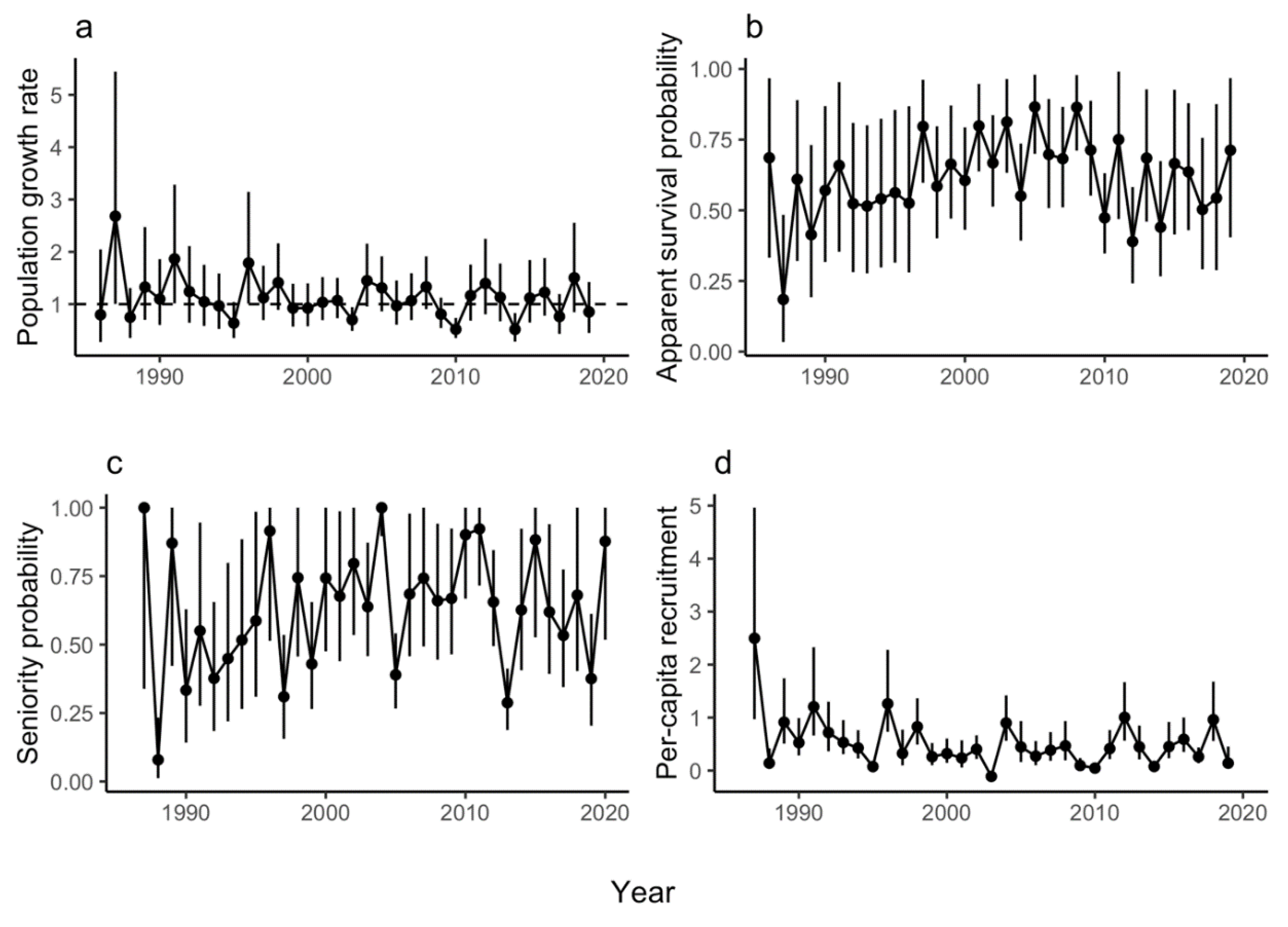
Figure 3.
Lily Pond: Posterior parameter distribution for each covariate included in models of (a) population growth rate and (b) survival. Shaded gray areas indicate the 95% credible intervals and solid lines within the posterior indicate the median value of the coefficient estimates. We considered a covariate to be significant if the 95% credible interval did not overlap zero.
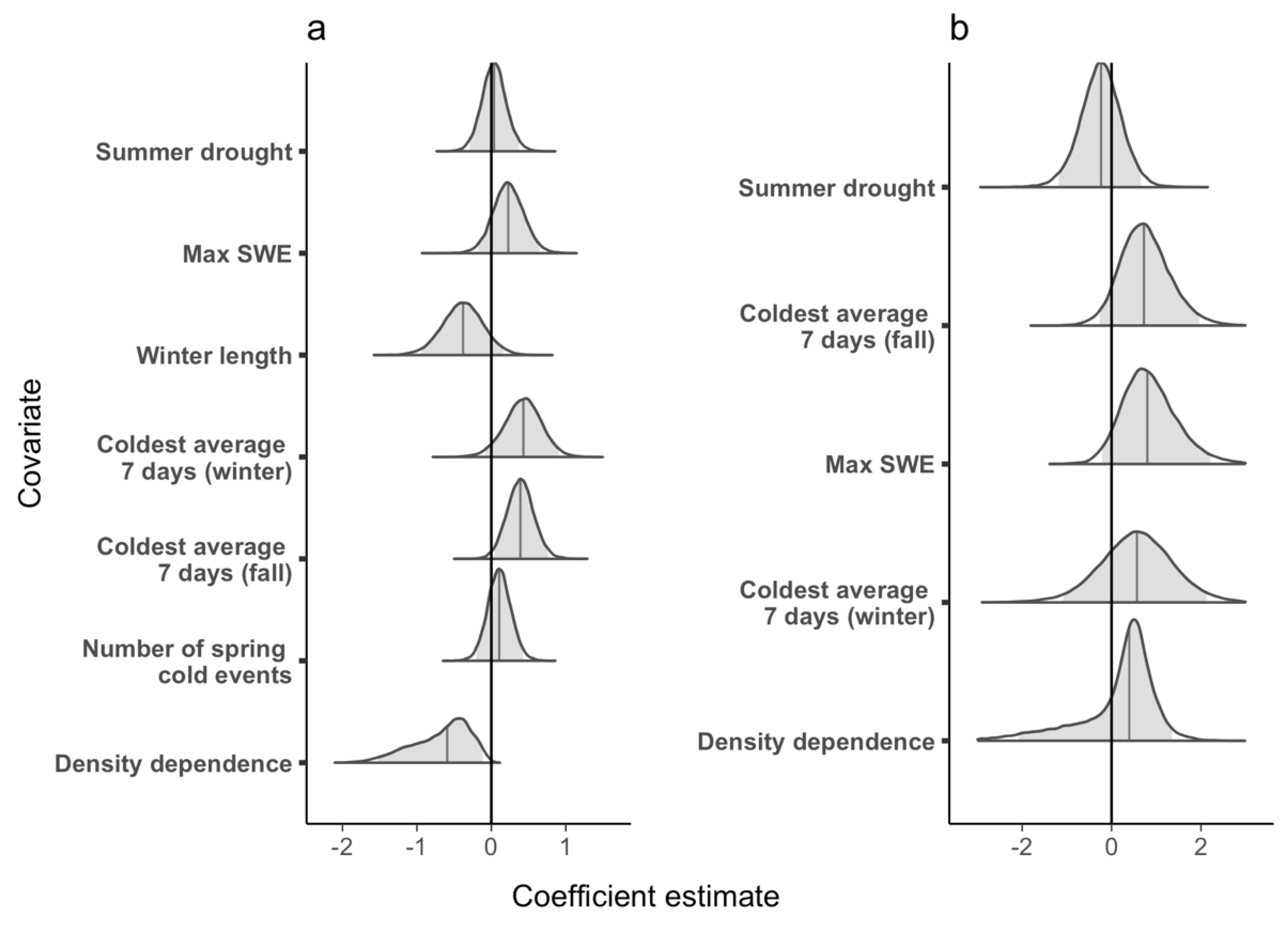
Figure 4.
Matthews Pond: Annual estimates and 95% credible intervals (CI) of (a) population growth rate (ρ) where the horizontal dashed line represents a stable population (i.e., growth rate of one), (b) mean survival probability (φ), (c) mean seniority probability (γ), and (d) per-capita recruitment.
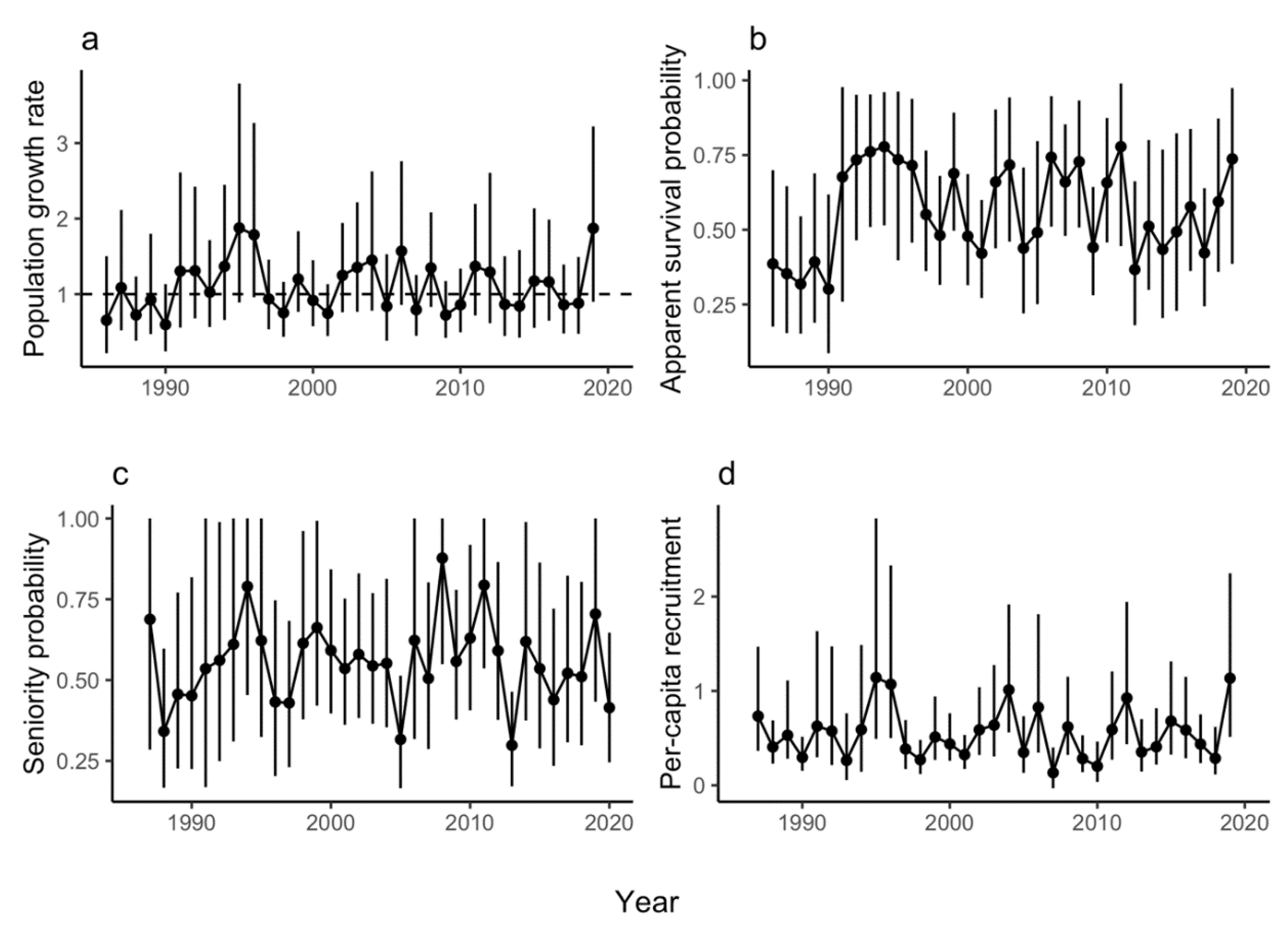
Figure 5.
Matthews Pond: Posterior parameter distribution for each covariate included in models of (a) population growth rate and (b) survival. Shaded gray areas indicate the 95% credible intervals and solid lines within the posterior indicate the median value of the coefficient estimates. We considered a covariate significant if the 95% credible interval did not overlap zero.

Table 1.
Description of covariate derivations and our hypotheses for the effects on population growth rate (ρ) and apparent survival probability (φ). ‘NA’ indicates that the covariate was not included in the model. Parentheticals in the covariate column indicate how the term was written in the model (e.g., Equations (1) and (2) in text). SWE = snow water equivalents and is a measure of snowpack. PHDI = Palmer Hydrologic Drought Index.
| Covariate | Derivation | Hypothesis (ρ) | Hypothesis (φ) |
|---|---|---|---|
| Density dependence (Pi) | The number of individuals at time i relative to the number of individuals in the population at time 2 (Ni/N2). | Population growth rate decreases as population size increases due to competition for resources via decreased recruitment or decreased survival. | Apparent survival decreases as population sizes increase due to competition for resources via increased mortality of adults or permanent emigration. |
| Number of spring cold events (sprevnt) | The total number of times that the minimum temperature was below −2 °C for 1 or more days after SWE was 50% of maximum for the year. | Increasing numbers of freezing events in the spring (e.g., early in the active season) increases mortality at multiple life stages decreasing recruitment and subsequently population growth rate. | NA |
| Coldest average 7 days in the fall (tmin7FL) | The coldest week (i.e., 7 day period) between October 1 and the development of persistent snow (SWE> = 2). | Colder temperatures in the fall (e.g., late in the active season) increase mortality at multiple life stages decreasing recruitment and subsequently population growth rate. | Colder temperatures in the fall (e.g., late in the active season) increase mortality at the adult stage. |
| Coldest average 7 days in the winter (tmin7wn) | The coldest week (i.e., 7-day period) between October 1 and March 31 | Colder temperatures in the winter increase mortality at multiple life stages decreasing recruitment and subsequently population growth rate. | Colder temperatures in the winter increase mortality at the adult stage. |
| Winter Length (winlength) | The number of days between persistent snowpack (Snow Water Equivalent (SWE)> = 2) and 50% of maximum SWE in the spring | Longer winters decrease recruitment (and subsequently population growth rate) because sub-adults may not have the resources to sustain them through the season. | Longer winters decrease survival because adults may not have the resources to sustain them through the season. |
| Maximum Snow Water Equivalent (maxswe) | The maximum SWE measurement for the breeding year. | Higher snowpack results in improved breeding conditions and summer habitat, resulting in increased recruitment and population growth rate. | Higher snowpack results in improved breeding conditions and summer habitat, resulting in increased survival. |
| Summer Drought (phdism) | PHDI value for estimating the month of metamorphosis (50 days past 50% of maximum SWE). | Increased summer drought results in decreased water availability on the landscape and increased mortality (via desiccation) at multiple life stages, reducing recruitment and population growth rate. | Increased summer drought results in decreased water availability on the landscape and increased mortality (via desiccation) at multiple life stages, adult survival. |
| Active season length (actseas) | The number of days between 50% of max SWE and the earliest date on which minimum temperature drops below −2 °C at the end of the growing season prior to the current breeding season (e.g., we used the active season in 2019 as a covariate on rho/phi in 2020). | Longer growing seasons increase recruitment/growth rate because individuals have more time to procure fat reserves prior to hibernation. | Longer growing seasons increase adult survival because individuals have more time to procure fat reserves prior to hibernation. |
Publisher’s Note: MDPI stays neutral with regard to jurisdictional claims in published maps and institutional affiliations. |
© 2020 by the authors. Licensee MDPI, Basel, Switzerland. This article is an open access article distributed under the terms and conditions of the Creative Commons Attribution (CC BY) license (http://creativecommons.org/licenses/by/4.0/).
Share and Cite
MDPI and ACS Style
Kissel, A.M.; Tenan, S.; Muths, E. Density Dependence and Adult Survival Drive Dynamics in Two High Elevation Amphibian Populations. Diversity 2020, 12, 478. https://doi.org/10.3390/d12120478
AMA Style
Kissel AM, Tenan S, Muths E. Density Dependence and Adult Survival Drive Dynamics in Two High Elevation Amphibian Populations. Diversity. 2020; 12(12):478. https://doi.org/10.3390/d12120478
Chicago/Turabian StyleKissel, Amanda M., Simone Tenan, and Erin Muths. 2020. "Density Dependence and Adult Survival Drive Dynamics in Two High Elevation Amphibian Populations" Diversity 12, no. 12: 478. https://doi.org/10.3390/d12120478
Note that from the first issue of 2016, this journal uses article numbers instead of page numbers. See further details here.