Dimension Reduction and Clustering Models for Single-Cell RNA Sequencing Data: A Comparative Study

 , ,
, ,
Abstract
1. Introduction
2. Results
2.1. Datasets
2.2. Measurements
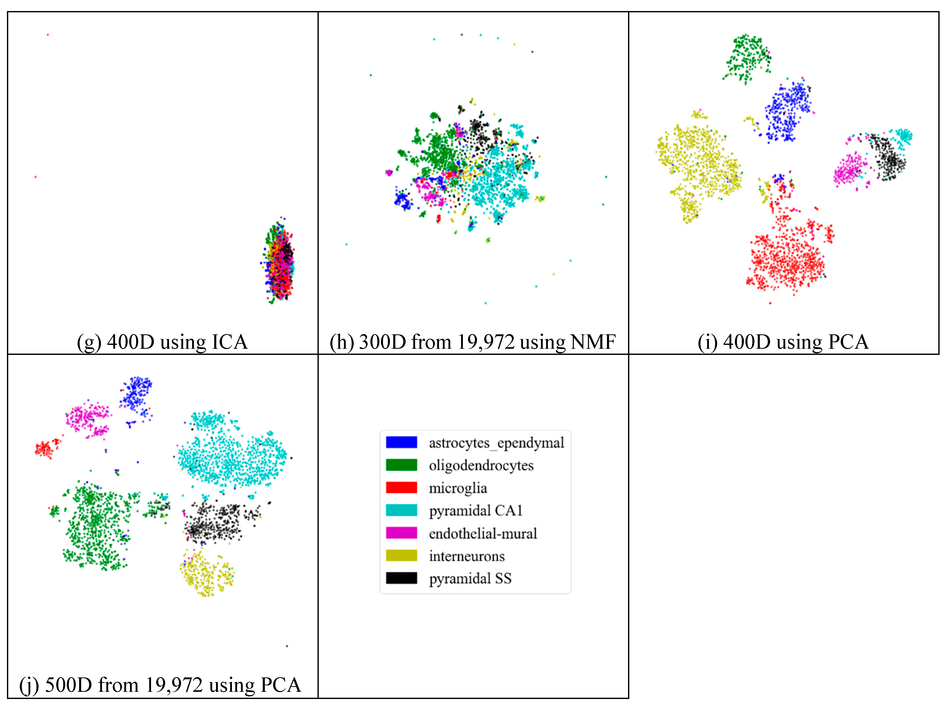
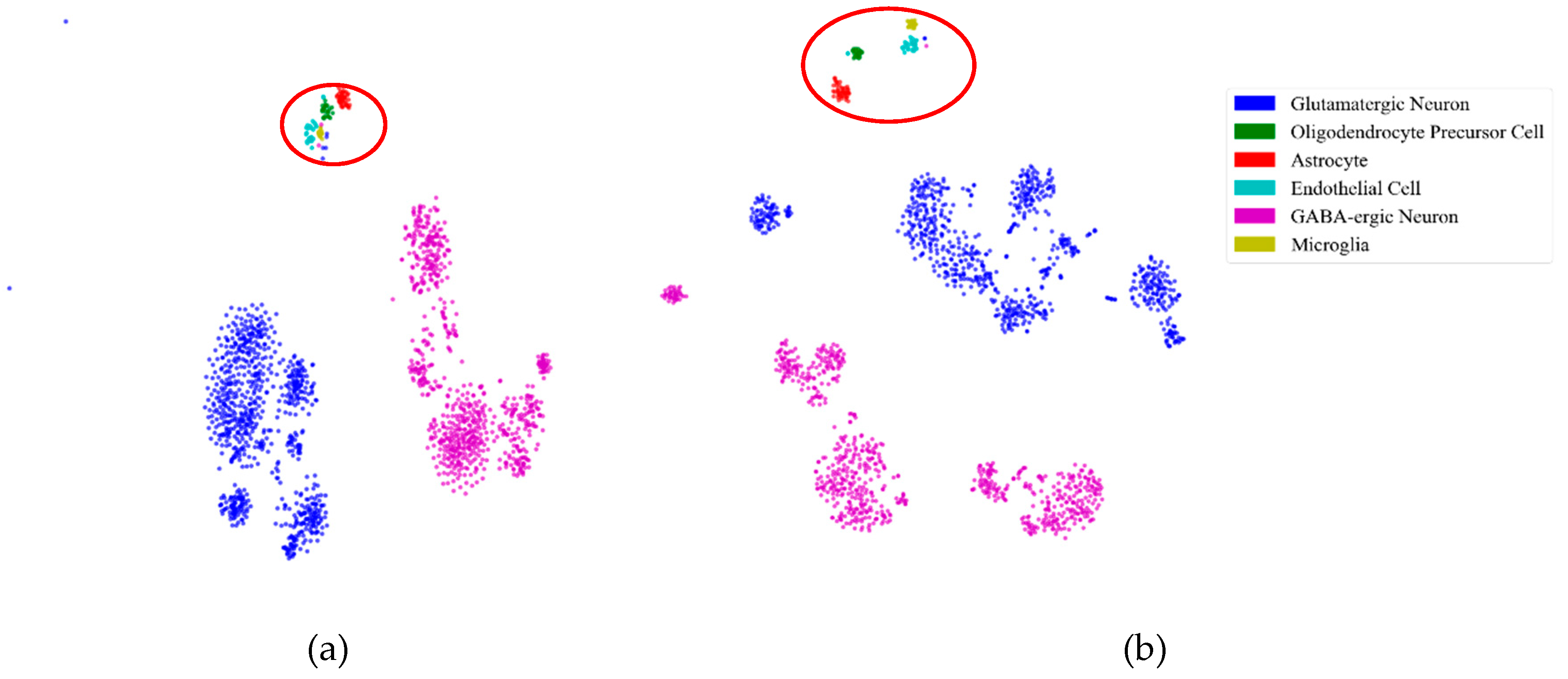
2.3. Visualization
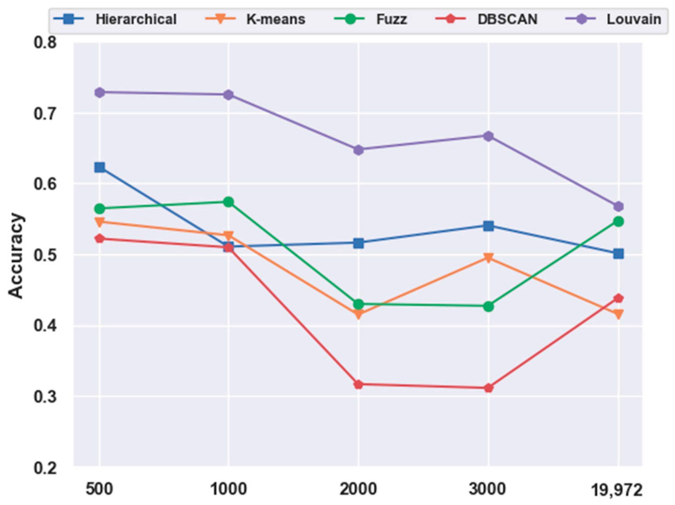
2.4. Analyses of Mouse Cortex Data Results
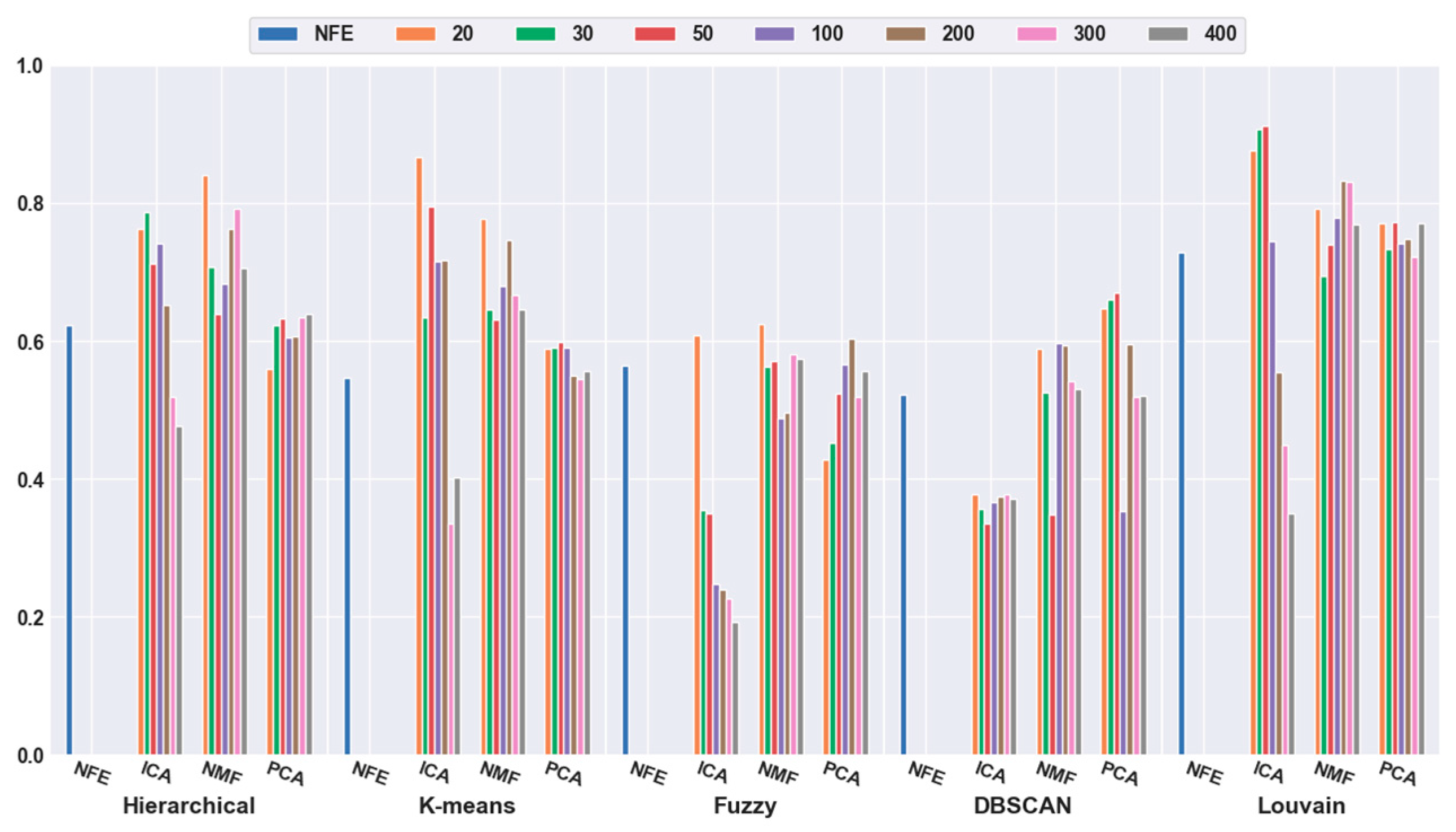
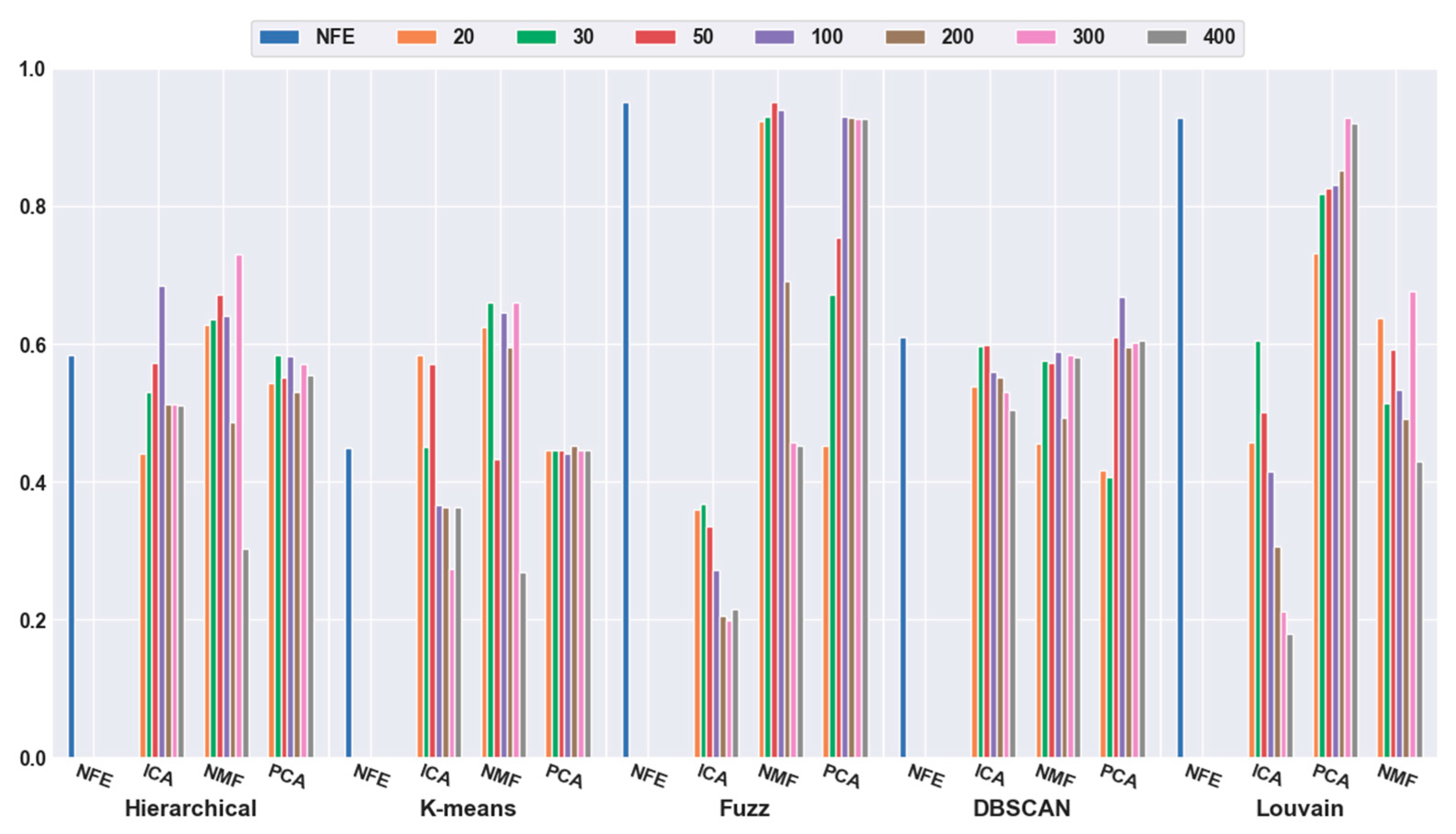
2.4.1. Effectiveness of Feature Selection
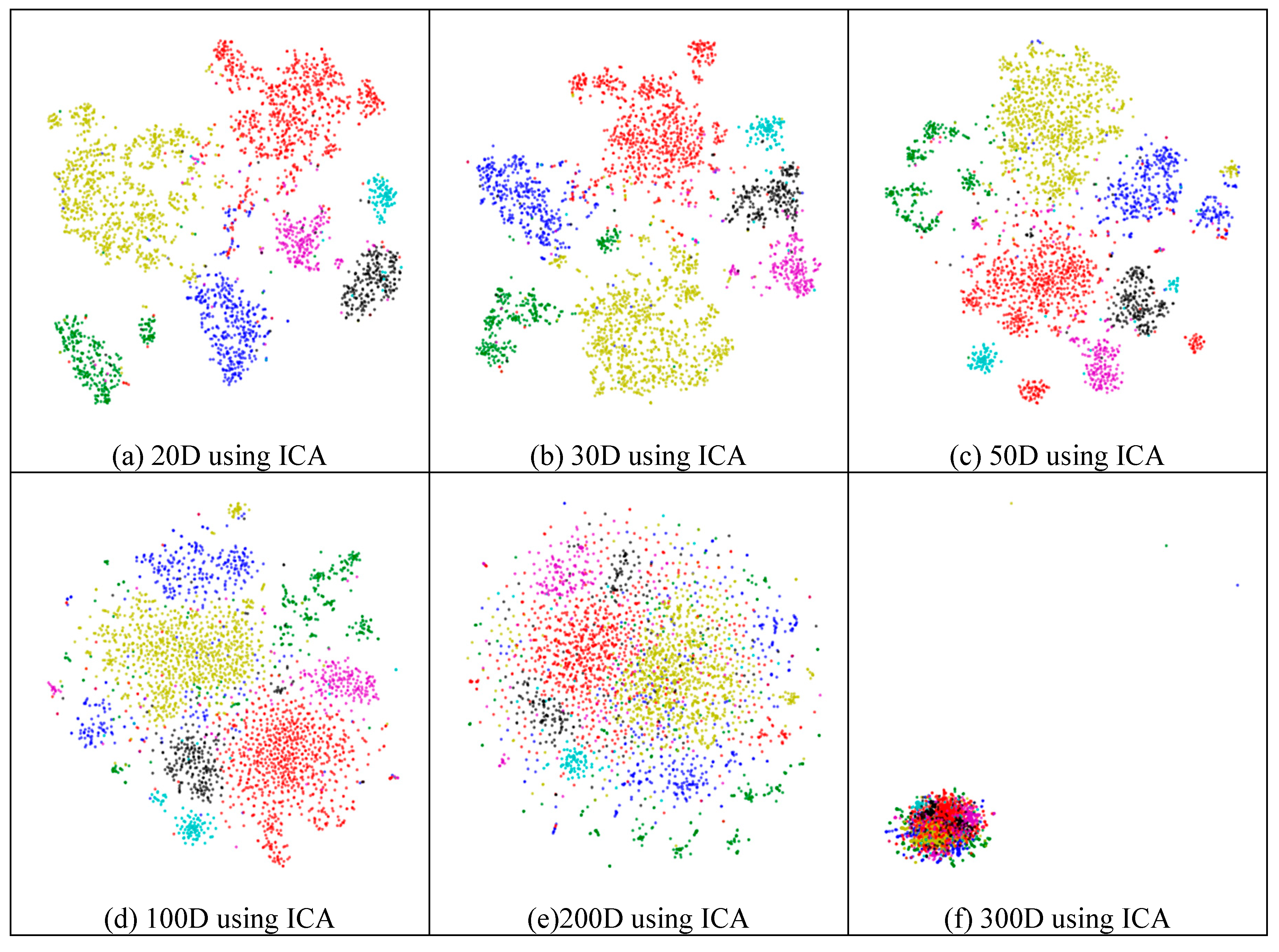
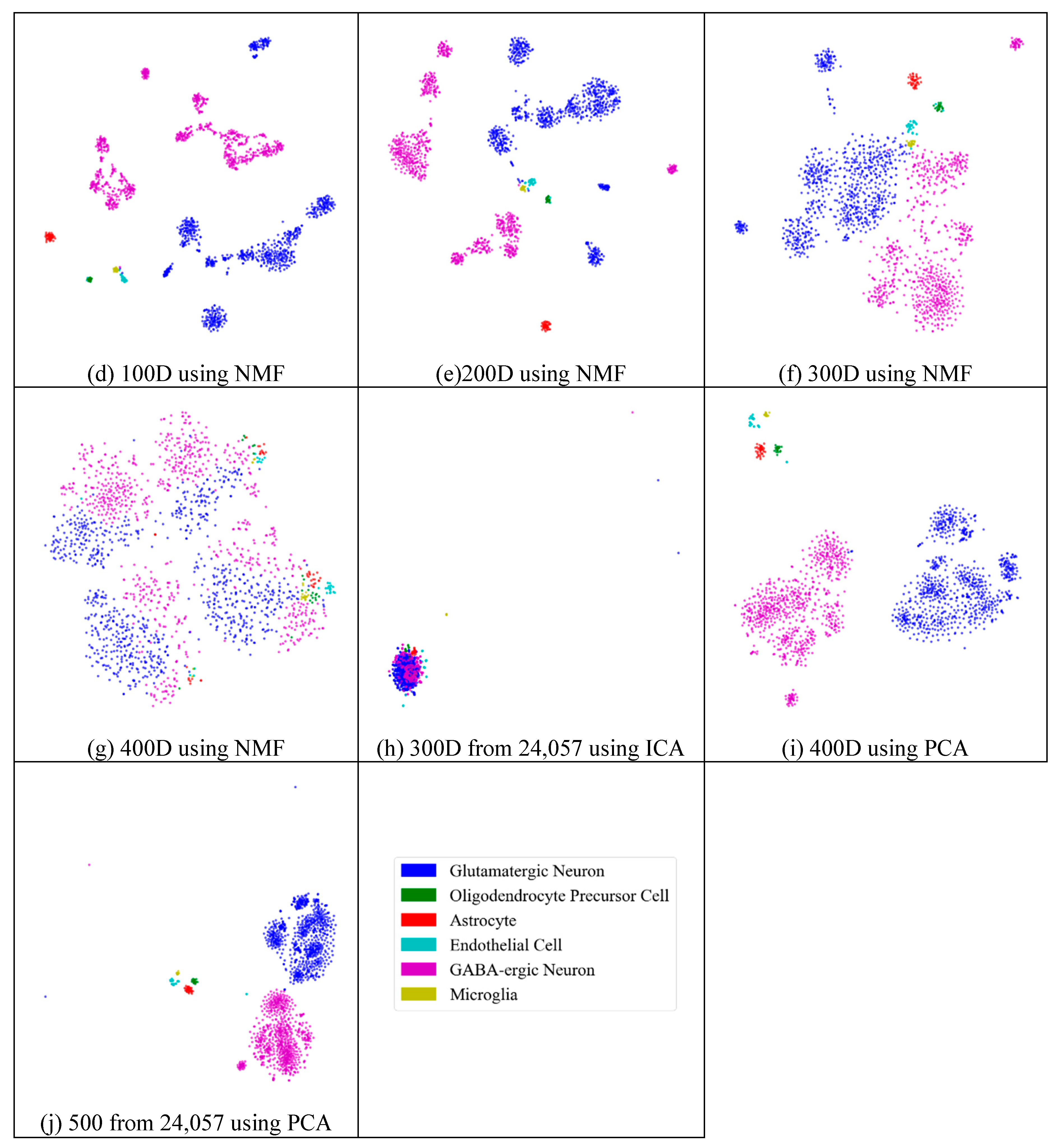
2.4.2. Effectiveness of Feature Extraction
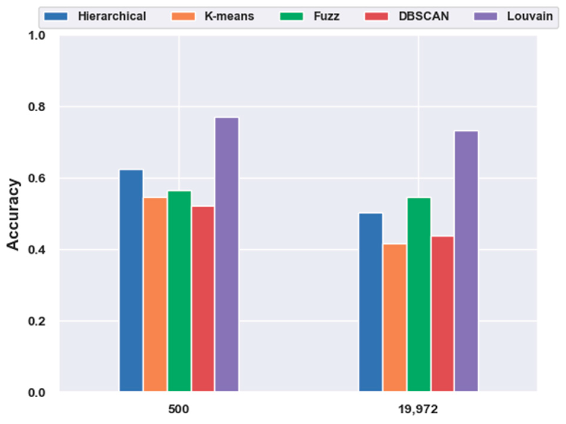
2.4.3. Which Clustering Algorithm Is Better?
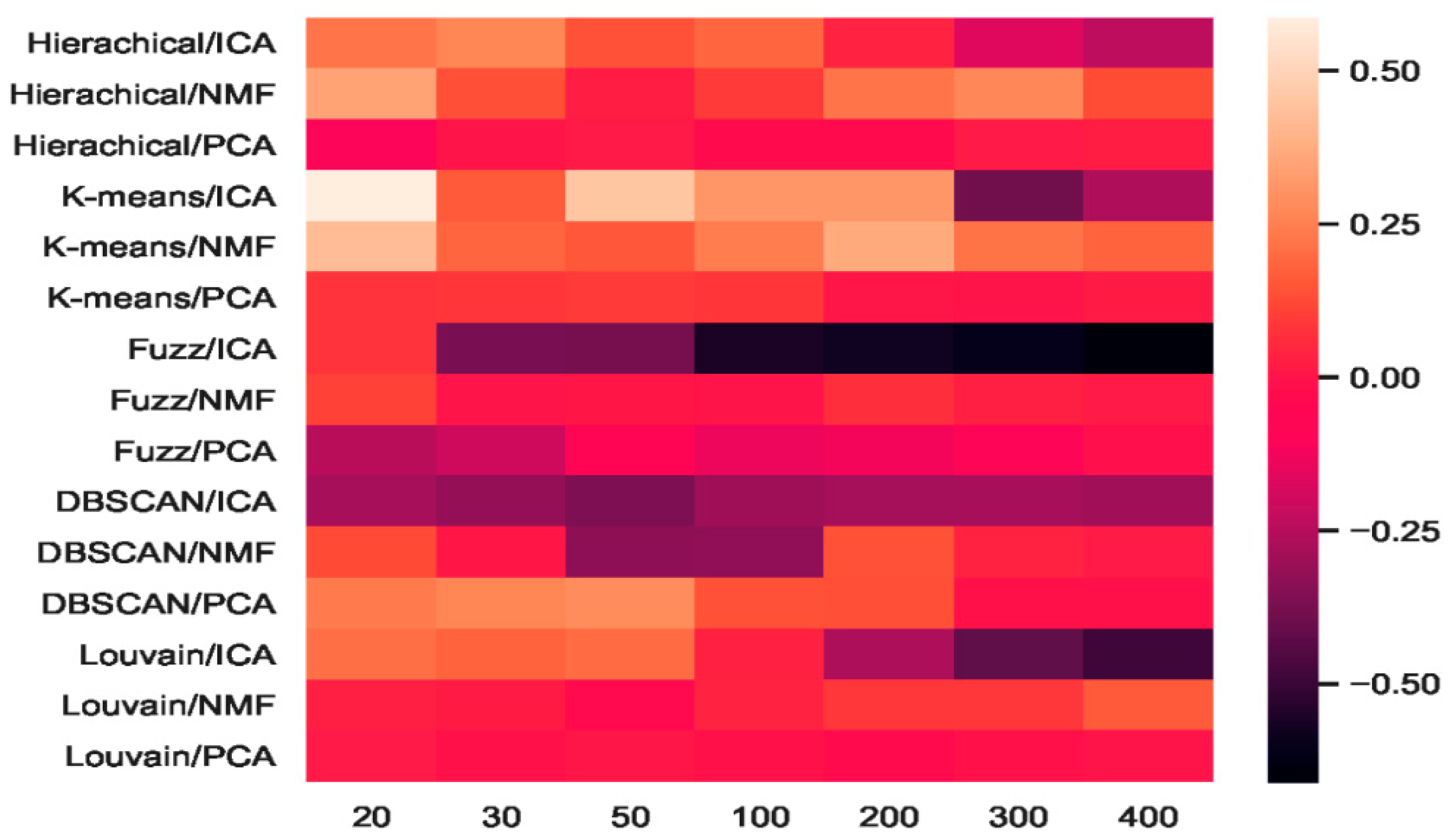
2.4.4. Which Combination Is Better?
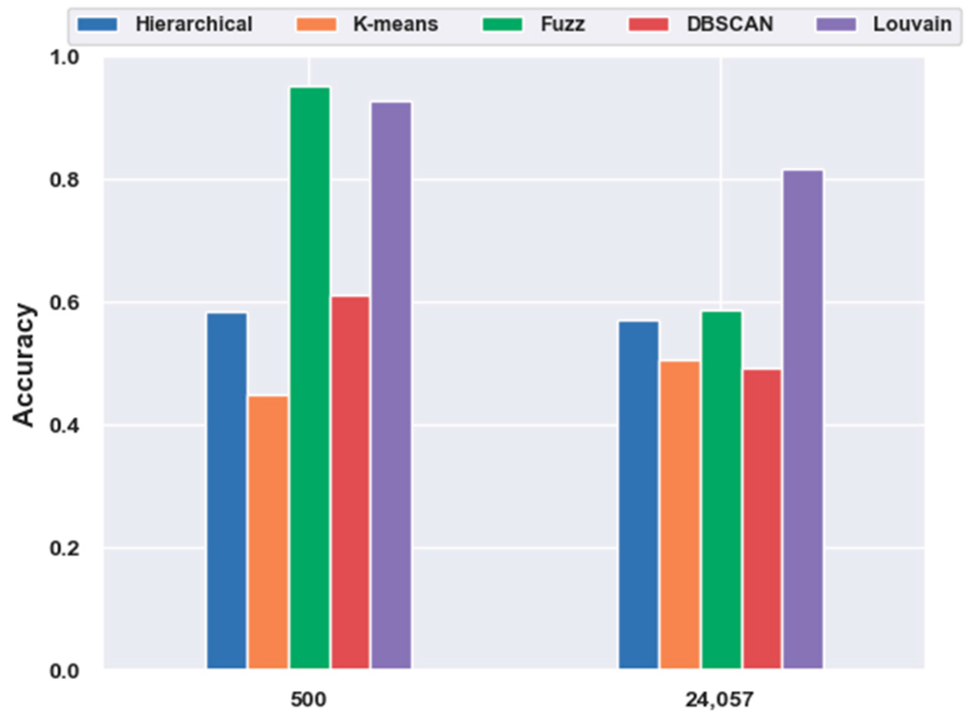
2.5. Analyses of Mouse Visual Cortex Data Results
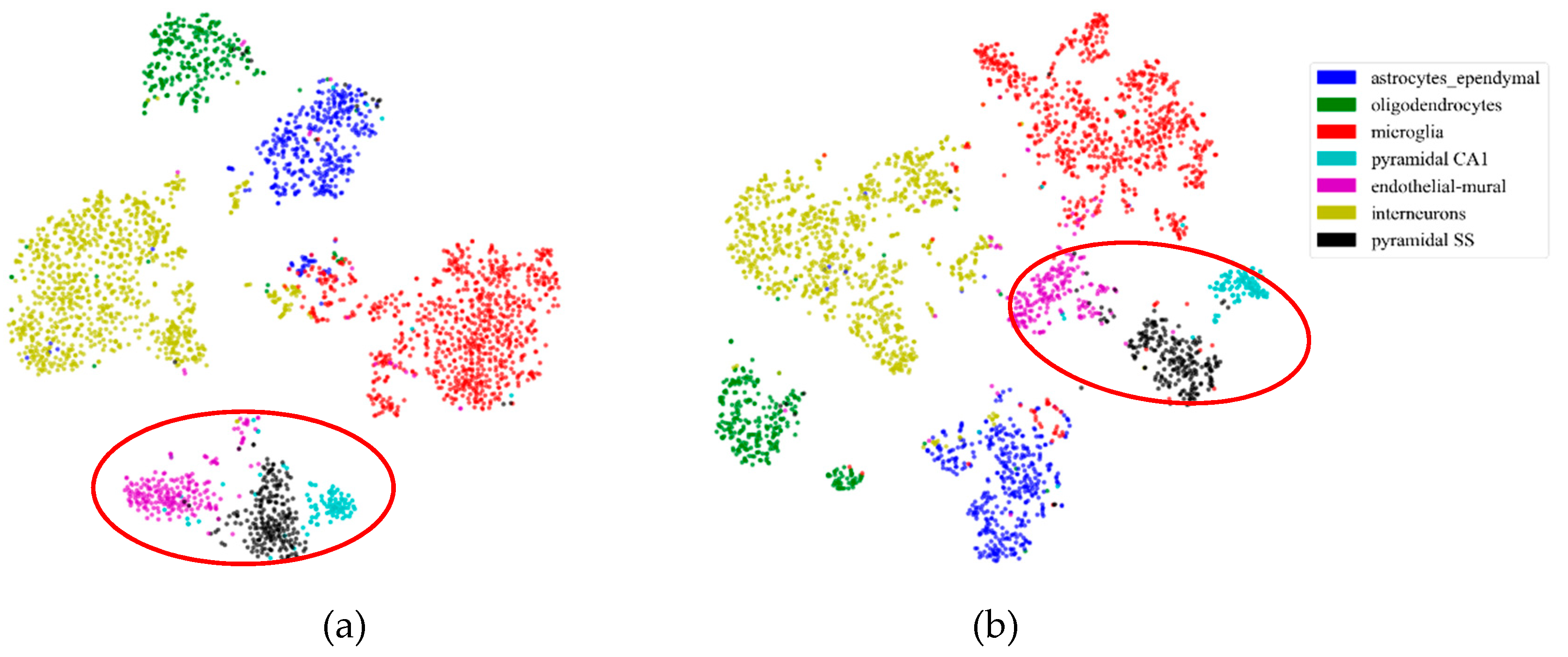
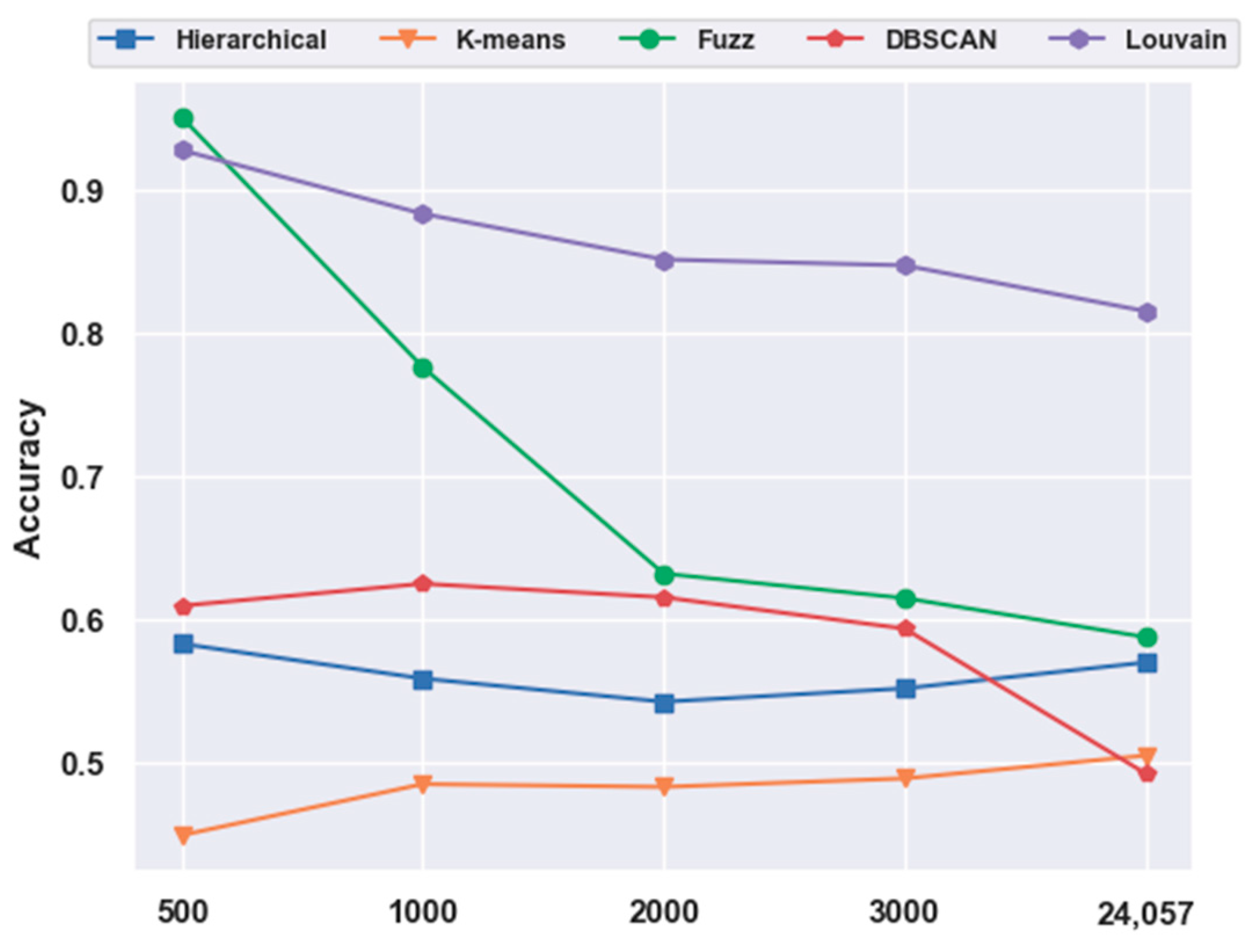
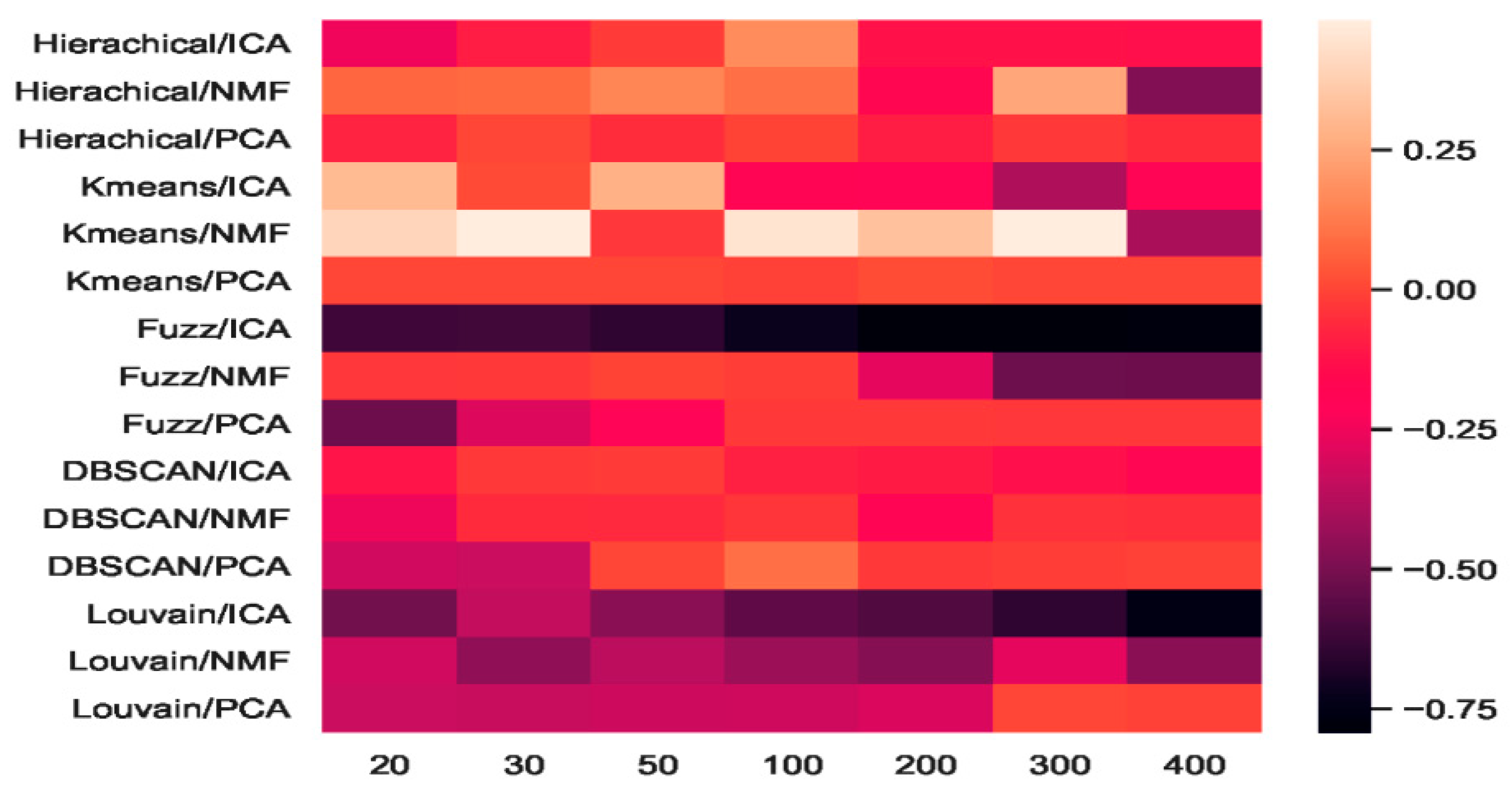
2.5.1. Consistency Results
2.5.2. Different Results
3. Discussion
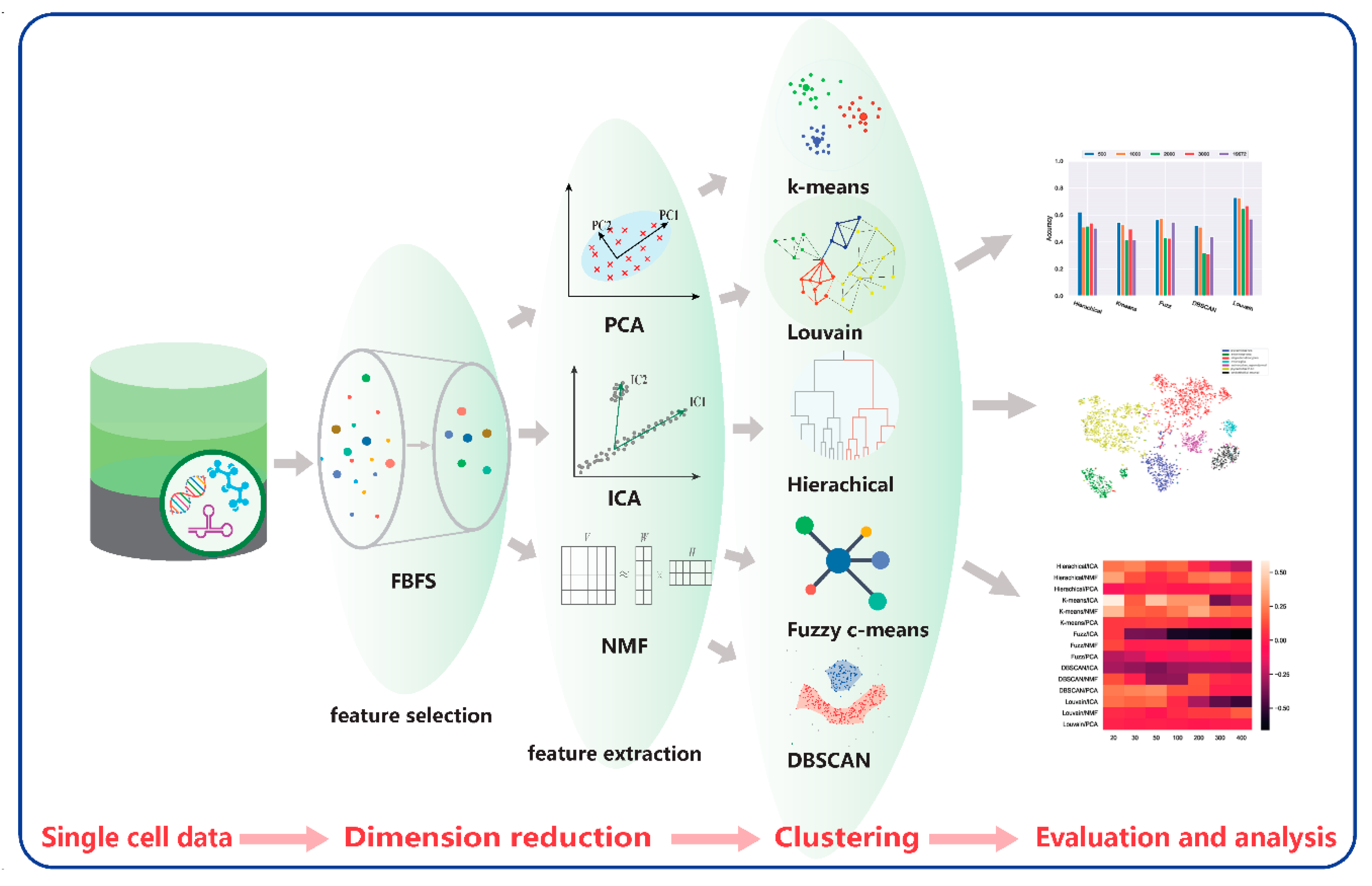
4. Materials and Methods
4.1. Dimensionality Reduction Models
4.2. Clustering Models
4.3. Comparative Framework
5. Conclusions
Author Contributions
Funding
Acknowledgments
Conflicts of Interest
References
- Chen, Y.; Li, P.; Huang, P.-H.; Xie, Y.; Mai, J.D.; Wang, L.; Nguyen, N.-T.; Huang, T.J. Rare cell isolation and analysis in microfluidics. Lab Chip 2014, 14, 626–645. [Google Scholar] [CrossRef] [PubMed]
- Zheng, C.; Zheng, L.; Yoo, J.-K.; Guo, H.; Zhang, Y.; Guo, X.; Kang, B.; Hu, R.; Huang, J.Y.; Zhang, Q.; et al. Landscape of infiltrating T cells in liver cancer revealed by single-cell sequencing. Cell 2017, 169, 1342–1356.e16. [Google Scholar] [CrossRef] [PubMed]
- Guo, X.; Zhang, Y.; Zheng, L.; Zheng, C.; Song, J.; Zhang, Q.; Kang, B.; Liu, Z.; Jin, L.; Xing, R.; et al. Global characterization of T cells in non-small-cell lung cancer by single-cell sequencing. Nat. Med. 2018, 24, 978–985. [Google Scholar] [CrossRef] [PubMed]
- Kiselev, V.Y.; Andrews, T.S.; Hemberg, M. Challenges in unsupervised clustering of single-cell RNA-seq data. Nat. Rev. Genet. 2019, 20, 273–282. [Google Scholar] [CrossRef] [PubMed]
- Regev, A.; Teichmann, S.A.; Lander, E.S.; Amit, I.; Benoist, C.; Birney, E.; Bodenmiller, B.; Campbell, P.; Carninci, P.; Clatworthy, M.; et al. The human cell atlas. eLife 2017, 6, e27041. [Google Scholar] [CrossRef]
- Wagner, A.; Regev, A.; Yosef, N. Revealing the vectors of cellular identity with single-cell genomics. Nat. Biotechnol. 2016, 34, 1145–1160. [Google Scholar] [CrossRef]
- Gao, Y.; Chuai, G.; Yu, W.; Qu, S.; Liu, Q. Data imbalance in CRISPR off-target prediction. Brief. Bioinform. 2019. [Google Scholar] [CrossRef]
- Sorzano, C.O.S.; Vargas, J.; Montano, A.P. A survey of dimensionality reduction techniques. arXiv 2014, arXiv:1403.2877. [Google Scholar]
- Dong, C.; Jin, Y.-T.; Hua, H.-L.; Wen, Q.-F.; Luo, S.; Zheng, W.-X.; Guo, F.-B. Comprehensive review of the identification of essential genes using computational methods: Focusing on feature implementation and assessment. Brief. Bioinform. 2020, 21, 171–181. [Google Scholar] [CrossRef]
- Wu, X.; Kumar, V.; Ross Quinlan, J.; Ghosh, J.; Yang, Q.; Motoda, H.; McLachlan, G.J.; Ng, A.; Liu, B.; Yu, P.S.; et al. Top 10 algorithms in data mining. Knowl. Inf. Syst. 2008, 14, 1–37. [Google Scholar] [CrossRef]
- Qiu, X.; Hill, A.; Packer, J.; Lin, D.; Ma, Y.-A.; Trapnell, C. Single-cell mRNA quantification and differential analysis with Census. Nat. Methods 2017, 14, 309–315. [Google Scholar] [CrossRef] [PubMed]
- Zeisel, A.; Muñoz-Manchado, A.B.; Codeluppi, S.; Lönnerberg, P.; Manno, G.L.; Juréus, A.; Marques, S.; Munguba, H.; He, L.; Betsholtz, C.; et al. Cell types in the mouse cortex and hippocampus revealed by single-cell RNA-seq. Science 2015, 347, 1138–1142. [Google Scholar] [CrossRef] [PubMed]
- žurauskienė, J.; Yau, C. pcaReduce: Hierarchical clustering of single cell transcriptional profiles. BMC Bioinform. 2016, 17, 140. [Google Scholar] [CrossRef] [PubMed]
- Duch, J.; Arenas, A. Community detection in complex networks using extremal optimization. Phys. Rev. E 2005, 72, 027104. [Google Scholar] [CrossRef]
- Fortunato, S.; Hric, D. Community detection in networks: A user guide. Phys. Rep. 2016, 659, 1–44. [Google Scholar] [CrossRef]
- Guerrero, M.; Montoya, F.G.; Baños, R.; Alcayde, A.; Gil, C. Adaptive community detection in complex networks using genetic algorithms. Neurocomputing 2017, 266, 101–113. [Google Scholar] [CrossRef]
- Blondel, V.D.; Guillaume, J.-L.; Lambiotte, R.; Lefebvre, E. Fast unfolding of communities in large networks. J. Stat. Mech. 2008, 2008, P10008. [Google Scholar] [CrossRef]
- Wolf, F.A.; Angerer, P.; Theis, F.J. SCANPY: Large-scale single-cell gene expression data analysis. Genome Biol. 2018, 19, 15. [Google Scholar] [CrossRef]
- Tasic, B.; Menon, V.; Nguyen, T.N.; Kim, T.K.; Jarsky, T.; Yao, Z.; Levi, B.; Gray, L.T.; Sorensen, S.A.; Dolbeare, T.; et al. Adult mouse cortical cell taxonomy revealed by single cell transcriptomics. Nat. Neurosci. 2016, 19, 335–346. [Google Scholar] [CrossRef]
- Prabhakaran, S.; Azizi, E.; Carr, A.; Pe’er, D. Dirichlet process mixture model for correcting technical variation in single-cell gene expression data. JMLR Workshop Conf. Proc. 2016, 48, 1070–1079. [Google Scholar]
- Shahnaz, F.; Berry, M.W.; Pauca, V.P.; Plemmons, R.J. Document clustering using nonnegative matrix factorization. Inf. Process. Manag. 2006, 42, 373–386. [Google Scholar] [CrossRef]
- Van der Maaten, L.; Hinton, G. Visualizing data using t-SNE. J. Mach. Learn. Res. 2008, 9, 2579–2605. [Google Scholar]
- Roweis, S.T.; Saul, L.K. Nonlinear dimensionality reduction by locally linear embedding. Science 2000, 290, 2323–2326. [Google Scholar] [CrossRef] [PubMed]
- Zech, J.; Pain, M.; Titano, J.; Badgeley, M.; Schefflein, J.; Su, A.; Costa, A.; Bederson, J.; Lehar, J.; Oermann, E.K. Natural language-based machine learning models for the annotation of clinical radiology reports. Radiology 2018, 287, 570–580. [Google Scholar] [CrossRef]
- Li, W.; Cerise, J.E.; Yang, Y.; Han, H. Application of t-SNE to human genetic data. J. Bioinform. Comput. Biol. 2017, 15, 1750017. [Google Scholar] [CrossRef]
- Abdelmoula, W.M.; Balluff, B.; Englert, S.; Dijkstra, J.; Reinders, M.J.T.; Walch, A.; McDonnell, L.A.; Lelieveldt, B.P.F. Data-driven identification of prognostic tumor subpopulations using spatially mapped t-SNE of mass spectrometry imaging data. Proc. Natl. Acad. Sci. USA 2016, 113, 12244–12249. [Google Scholar] [CrossRef]
- Pudil, P.; Novovičová, J. Novel methods for feature subset selection with respect to problem knowledge. In Feature Extraction, Construction and Selection; Liu, H., Motoda, H., Eds.; Springer: Boston, MA, USA, 1998; pp. 101–116. [Google Scholar]
- Guyon, I.; Elisseeff, A. An introduction to variable and feature selection. J. Mach. Learn. Res. 2003, 3, 1157–1182. [Google Scholar]
- Wang, D.; Liang, Y.; Xu, D.; Feng, X.; Guan, R. A content-based recommender system for computer science publications. Knowl. Based Syst. 2018, 157, 1–9. [Google Scholar] [CrossRef]
- Jolliffe, I. Principal component analysis. In International Encyclopedia of Statistical Science; Lovric, M., Ed.; Springer: Berlin/Heidelberg, Germany, 2011; pp. 1094–1096. [Google Scholar]
- Buettner, F.; Moignard, V.; Göttgens, B.; Theis, F.J. Probabilistic PCA of censored data: Accounting for uncertainties in the visualization of high-throughput single-cell qPCR data. Bioinformatics 2014, 30, 1867–1875. [Google Scholar] [CrossRef]
- Hyvärinen, A.; Oja, E. Independent component analysis: Algorithms and applications. Neural Netw. 2000, 13, 411–430. [Google Scholar] [CrossRef]
- Pearlmutter, B.A.; Parra, L.C. Maximum likelihood blind source separation: A context-sensitive generalization of ICA. In Advances in Neural Information Processing Systems 9; Mozer, M.C., Jordan, M.I., Petsche, T., Eds.; MIT Press: Cambridge, MA, USA, 1997; pp. 613–619. [Google Scholar]
- Mitianoudis, N.; Stathaki, T. Pixel-based and region-based image fusion schemes using ICA bases. Inf. Fusion 2007, 8, 131–142. [Google Scholar] [CrossRef]
- Lee, J.-H.; Jung, H.-Y.; Lee, T.-W.; Lee, S.-Y. Speech feature extraction using independent component analysis. In Proceedings of the 2000 IEEE International Conference on Acoustics, Speech, and Signal Processing. Proceedings (Cat. No.00CH37100), Istanbul, Turkey, 5–9 June 2000; Volume 3, pp. 1631–1634. [Google Scholar]
- Scholz, M.; Gatzek, S.; Sterling, A.; Fiehn, O.; Selbig, J. Metabolite fingerprinting: Detecting biological features by independent component analysis. Bioinformatics 2004, 20, 2447–2454. [Google Scholar] [CrossRef] [PubMed]
- Lee, D.D.; Seung, H.S. Learning the parts of objects by non-negative matrix factorization. Nature 1999, 401, 788–791. [Google Scholar] [CrossRef] [PubMed]
- Zhang, T.; Fang, B.; Tang, Y.Y.; He, G.; Wen, J. Topology preserving non-negative matrix factorization for face recognition. IEEE Trans. Image Process. 2008, 17, 574–584. [Google Scholar] [CrossRef]
- Schmidt, M.N.; Olsson, R.K. Single-channel speech separation using sparse non-negative matrix factorization. In Proceedings of the Ninth International Conference on Spoken Language Processing, Pittsburgh, PA, USA, 17–21 September 2006; pp. 2614–2617. [Google Scholar]
- Tresch, M.C.; Cheung, V.C.K.; d’Avella, A. Matrix factorization algorithms for the identification of muscle synergies: Evaluation on simulated and experimental data sets. J. Neurophysiol. 2006, 95, 2199–2212. [Google Scholar] [CrossRef]
- Wang, J.J.-Y.; Bensmail, H.; Gao, X. Multiple graph regularized nonnegative matrix factorization. Pattern Recognit. 2013, 46, 2840–2847. [Google Scholar] [CrossRef]
- Sun, L.; Ge, H.; Kang, W. Non-negative matrix factorization based modeling and training algorithm for multi-label learning. Front. Comput. Sci. 2019, 13, 1243–1254. [Google Scholar] [CrossRef]
- Sculley, D. Web-scale K-means clustering. In Proceedings of the 19th International Conference on World Wide Web, Raleigh, NC, USA, 26–30 April 2010; ACM: New York, NY, USA, 2010; pp. 1177–1178. [Google Scholar]
- Wagstaff, K.; Cardie, C.; Rogers, S.; Schroedl, S. Constrained K-means clustering with background knowledge. In Proceedings of the Eighteenth International Conference on Machine Learning, Williamstown, MA, USA, 28 June–1 July 2001; Morgan Kaufmann: Burlington, MA, USA, 2001; pp. 577–584. [Google Scholar]
- Bezdek, J.C.; Ehrlich, R.; Full, W. FCM: The fuzzy C-means clustering algorithm. Comput. Geosci. 1984, 10, 191–203. [Google Scholar] [CrossRef]
- Ester, M.; Kriegel, H.-P.; Sander, J.; Xu, X. A density-based algorithm for discovering clusters a density-based algorithm for discovering clusters in large spatial databases with noise. In Proceedings of the Second International Conference on Knowledge Discovery and Data Mining, Oregon, Portland, 2–4 August 1996; AAAI Press: Palo Alto, CA, USA, 1996; pp. 226–231. [Google Scholar]
- Lancichinetti, A.; Fortunato, S. Community detection algorithms: A comparative analysis. Phys. Rev. E 2009, 80, 056117. [Google Scholar] [CrossRef]
- Kiselev, V.Y.; Kirschner, K.; Schaub, M.T.; Andrews, T.; Yiu, A.; Chandra, T.; Natarajan, K.N.; Reik, W.; Barahona, M.; Green, A.R.; et al. SC3: Consensus clustering of single-cell RNA-seq data. Nat. Methods 2017, 14, 483–486. [Google Scholar] [CrossRef]
- Zheng, G.X.Y.; Terry, J.M.; Belgrader, P.; Ryvkin, P.; Bent, Z.W.; Wilson, R.; Ziraldo, S.B.; Wheeler, T.D.; McDermott, G.P.; Zhu, J.; et al. Massively parallel digital transcriptional profiling of single cells. Nat. Commun. 2017, 8, 1–12. [Google Scholar] [CrossRef] [PubMed]
- Grün, D.; Lyubimova, A.; Kester, L.; Wiebrands, K.; Basak, O.; Sasaki, N.; Clevers, H.; van Oudenaarden, A. Single-cell messenger RNA sequencing reveals rare intestinal cell types. Nature 2015, 525, 251–255. [Google Scholar] [CrossRef] [PubMed]
- Darmanis, S.; Sloan, S.A.; Zhang, Y.; Enge, M.; Caneda, C.; Shuer, L.M.; Gephart, M.G.H.; Barres, B.A.; Quake, S.R. A survey of human brain transcriptome diversity at the single cell level. Proc. Natl. Acad. Sci. USA 2015, 112, 7285–7290. [Google Scholar] [CrossRef] [PubMed]
- Guo, M.; Wang, H.; Potter, S.S.; Whitsett, J.A.; Xu, Y. SINCERA: A pipeline for single-Cell RNA-Seq profiling analysis. PLoS Comput. Biol. 2015, 11, e1004575. [Google Scholar] [CrossRef] [PubMed]
- Yan, L.; Yang, M.; Guo, H.; Yang, L.; Wu, J.; Li, R.; Liu, P.; Lian, Y.; Zheng, X.; Yan, J.; et al. Single-cell RNA-Seq profiling of human preimplantation embryos and embryonic stem cells. Nat. Struct. Mol. Biol. 2013, 20, 1131–1139. [Google Scholar] [CrossRef] [PubMed]
- Levine, J.H.; Simonds, E.F.; Bendall, S.C.; Davis, K.L.; Amir, E.D.; Tadmor, M.D.; Litvin, O.; Fienberg, H.G.; Jager, A.; Zunder, E.R.; et al. Data-driven phenotypic dissection of AML reveals progenitor-like cells that correlate with prognosis. Cell 2015, 162, 184–197. [Google Scholar] [CrossRef]
- Mallik, S.; Zhao, Z. Multi-objective optimized fuzzy clustering for detecting cell clusters from single-cell expression profiles. Genes 2019, 10, 611. [Google Scholar] [CrossRef]
- Zhang, Q.; Liu, W.; Liu, C.; Lin, S.-Y.; Guo, A.-Y. SEGtool: A specifically expressed gene detection tool and applications in human tissue and single-cell sequencing data. Brief. Bioinform. 2018, 19, 1325–1336. [Google Scholar] [CrossRef]
- Ye, X.; Ho, J.W.K. Ultrafast clustering of single-cell flow cytometry data using FlowGrid. BMC Syst. Biol. 2019, 13, 35. [Google Scholar] [CrossRef]
- Yang, L.; Liu, J.; Lu, Q.; Riggs, A.D.; Wu, X. SAIC: An iterative clustering approach for analysis of single cell RNA-seq data. BMC Genom. 2017, 18, 689. [Google Scholar] [CrossRef]
- Xue, Z.; Huang, K.; Cai, C.; Cai, L.; Jiang, C.; Feng, Y.; Liu, Z.; Zeng, Q.; Cheng, L.; Sun, Y.E.; et al. Genetic programs in human and mouse early embryos revealed by single-cell RNA sequencing. Nature 2013, 500, 593–597. [Google Scholar] [CrossRef] [PubMed]
- Treutlein, B.; Brownfield, D.G.; Wu, A.R.; Neff, N.F.; Mantalas, G.L.; Espinoza, F.H.; Desai, T.J.; Krasnow, M.A.; Quake, S.R. Reconstructing lineage hierarchies of the distal lung epithelium using single-cell RNA-seq. Nature 2014, 509, 371–375. [Google Scholar] [CrossRef] [PubMed]
- Sun, Z.; Wang, C.-Y.; Lawson, D.A.; Kwek, S.; Velozo, H.G.; Owyong, M.; Lai, M.-D.; Fong, L.; Wilson, M.; Su, H.; et al. Single-cell RNA sequencing reveals gene expression signatures of breast cancer-associated endothelial cells. Oncotarget 2017, 9, 10945–10961. [Google Scholar] [CrossRef] [PubMed]
- Shekhar, K.; Lapan, S.W.; Whitney, I.E.; Tran, N.M.; Macosko, E.Z.; Kowalczyk, M.; Adiconis, X.; Levin, J.Z.; Nemesh, J.; Goldman, M.; et al. Comprehensive classification of retinal bipolar neurons by single-cell transcriptomics. Cell 2016, 166, 1308–1323.e30. [Google Scholar] [CrossRef] [PubMed]
- Macosko, E.Z.; Basu, A.; Satija, R.; Nemesh, J.; Shekhar, K.; Goldman, M.; Tirosh, I.; Bialas, A.R.; Kamitaki, N.; Martersteck, E.M.; et al. Highly parallel genome-wide expression profiling of individual cells using nanoliter droplets. Cell 2015, 161, 1202–1214. [Google Scholar] [CrossRef]
- Kakushadze, Z.; Yu, W. *K-means and cluster models for cancer signatures. Biomol. Detect. Quantif. 2017, 13, 7–31. [Google Scholar] [CrossRef]
- Jung, M.; Wells, D.; Rusch, J.; Ahmad, S.; Marchini, J.; Myers, S.R.; Conrad, D.F. Unified single-cell analysis of testis gene regulation and pathology in five mouse strains. eLife 2019, 8, e43966. [Google Scholar] [CrossRef]
- Trapnell, C.; Cacchiarelli, D.; Grimsby, J.; Pokharel, P.; Li, S.; Morse, M.; Lennon, N.J.; Livak, K.J.; Mikkelsen, T.S.; Rinn, J.L. The dynamics and regulators of cell fate decisions are revealed by pseudotemporal ordering of single cells. Nat. Biotechnol. 2014, 32, 381–386. [Google Scholar] [CrossRef]
- Shin, J.; Berg, D.A.; Zhu, Y.; Shin, J.Y.; Song, J.; Bonaguidi, M.A.; Enikolopov, G.; Nauen, D.W.; Christian, K.M.; Ming, G.; et al. Single-cell RNA-seq with waterfall reveals molecular cascades underlying adult neurogenesis. Cell Stem Cell 2015, 17, 360–372. [Google Scholar] [CrossRef]
- Kubo, M.; Nishiyama, T.; Tamada, Y.; Sano, R.; Ishikawa, M.; Murata, T.; Imai, A.; Lang, D.; Demura, T.; Reski, R.; et al. Single-cell transcriptome analysis of Physcomitrella leaf cells during reprogramming using microcapillary manipulation. Nucleic Acids Res. 2019, 47, 4539–4553. [Google Scholar] [CrossRef]
- Angelidis, I.; Simon, L.M.; Fernandez, I.E.; Strunz, M.; Mayr, C.H.; Greiffo, F.R.; Tsitsiridis, G.; Ansari, M.; Graf, E.; Strom, T.-M.; et al. An atlas of the aging lung mapped by single cell transcriptomics and deep tissue proteomics. Nat. Commun. 2019, 10, 1–17. [Google Scholar] [CrossRef] [PubMed]


| Broad Type | Count |
|---|---|
| Astrocyte | 43 |
| Endothelial Cell | 29 |
| GABA-ergic Neuron | 761 |
| Glutamatergic Neuron | 812 |
| Microglia | 22 |
| Oligodendrocyte | 38 |
| Oligodendrocyte Precursor | 22 |
| Unclassified | 82 |
| Combination Numbers | Combination Mode | Field |
|---|---|---|
| 1 | K-Means | mouse retinal cells [48] peripheral blood mononuclear cell [49] |
| 2 | Hierarchical Clustering | intestinal cell types [50] adult brain cell [51] embryonic mouse lung [52] human preimplantation embryos and embryonic stem cells [53] |
| 3 | Louvain | progenitor-like cells [54] peripheral blood mononuclear cell [18] |
| 4 | Fuzzy C-Means | rare intestinal cell type in mice [55] Genotype-tissue Expression (GTEx) human tissue dataset [56] |
| 5 | DBSCAN 1 | B-cell Lymphoma [57] |
| 6 | PCA 2 + K-Means | intestinal cell types [50] Lung epithelial cells [58] |
| 7 | PCA + Hierarchical Clustering | human and mouse early embryo [59] distal lung epithelium [60] breast-cancer-associated endothelial cells [61] |
| 8 | PCA + Louvain | retinal bipolar neurons [62] |
| 9 | PCA + Fuzzy C-Means | rare intestinal cell type in mice [55] |
| 10 | PCA + DBSCAN | mouse retinal cells [63] |
| 11 | NMF 3 + K-Means | renal cell carcinoma, liver cancer, lung cancer [64] |
| 12 | NMF + Hierarchical Clustering | mouse strain [65] |
| 13 | NMF + Louvain | unreported model |
| 14 | NMF + Fuzzy C-Means | unreported model |
| 15 | NMF + DBSCAN | unreported model |
| 16 | ICA 4 + K-Means | individual cell [66] adult hippocampal quiescent neural stem cell [67] |
| 17 | ICA + Hierarchical Clustering | Physcomitrella leaf cell [68] |
| 18 | ICA + Louvain | human aging lung [69] |
| 19 | ICA + Fuzzy C-Means | unreported model |
| 20 | ICA + DBSCAN | unreported model |
© 2020 by the authors. Licensee MDPI, Basel, Switzerland. This article is an open access article distributed under the terms and conditions of the Creative Commons Attribution (CC BY) license (http://creativecommons.org/licenses/by/4.0/).
Share and Cite
Feng, C.; Liu, S.; Zhang, H.; Guan, R.; Li, D.; Zhou, F.; Liang, Y.; Feng, X. Dimension Reduction and Clustering Models for Single-Cell RNA Sequencing Data: A Comparative Study. Int. J. Mol. Sci. 2020, 21, 2181. https://doi.org/10.3390/ijms21062181
Feng C, Liu S, Zhang H, Guan R, Li D, Zhou F, Liang Y, Feng X. Dimension Reduction and Clustering Models for Single-Cell RNA Sequencing Data: A Comparative Study. International Journal of Molecular Sciences. 2020; 21(6):2181. https://doi.org/10.3390/ijms21062181
Chicago/Turabian StyleFeng, Chao, Shufen Liu, Hao Zhang, Renchu Guan, Dan Li, Fengfeng Zhou, Yanchun Liang, and Xiaoyue Feng. 2020. "Dimension Reduction and Clustering Models for Single-Cell RNA Sequencing Data: A Comparative Study" International Journal of Molecular Sciences 21, no. 6: 2181. https://doi.org/10.3390/ijms21062181
APA StyleFeng, C., Liu, S., Zhang, H., Guan, R., Li, D., Zhou, F., Liang, Y., & Feng, X. (2020). Dimension Reduction and Clustering Models for Single-Cell RNA Sequencing Data: A Comparative Study. International Journal of Molecular Sciences, 21(6), 2181. https://doi.org/10.3390/ijms21062181