Relationship between Visibility, Air Pollution Index and Annual Mortality Rate in Association with the Occurrence of Rainfall—A Probabilistic Approach

Abstract

An innovative method was proposed to facilitate the analyses of meteorological conditions and selected air pollution indices’ influence on visibility, air quality index and mortality. The constructed calculation algorithm is dedicated to simulating the visibility in a single episode, first of all. It was derived after applying logistic regression methodology. It should be stressed that eight visibility thresholds (Vis) were adopted in order to build proper classification models with a number of relevant advantages. At first, there exists the possibility to analyze the impact of independent variables on visibility with the consideration of its’ real variability. Secondly, through the application of the Monte Carlo method and the assumed classification algorithms, it was made possible to model the number of days during a precipitation and no-precipitation periods in a yearly cycle, on which the visibility ranged practically: Vis < 8; Vis = 8–12 km, Vis = 12–16 km, Vis = 16–20 km, Vis = 20–24 km, Vis = 24–28 km, Vis = 28–32 km, Vis > 32 km. The derived algorithm proved a particular role of precipitation and no-precipitation periods in shaping the air visibility phenomena. Higher visibility values and a lower number of days with increased visibility were found for the precipitation period contrary to no-precipitation one. The air quality index was lower for precipitation days, and moreover, strong, non-linear relationships were found between mortality and visibility, considering precipitation and seasonality effects.

1. Introduction

Ambient air pollution is one of the greatest environmental threats to human health and has been reported to be responsible for 4.2 million deaths worldwide in 2016 [1]. Visibility is a common atmospheric measurement that can serve as a visual indicator of air quality [2]. In addition, visibility is a useful proxy for assessing environmental health risks from ambient air pollution and evaluating the impact of air pollution on public health [3]. Research on the effects of visibility on human health is being increasingly often conducted around the world. Studies indicate that the exposure to the factors associated with poor atmospheric visibility was a contributing factor to increased risk of influenza infection [4] as well as higher respiratory and cardiovascular mortality [5].

The relationships between the COVID-19 pandemic and air pollution have been made evident. The data published by ESA and NASA have shown air pollution to be decreased as much as 30% in well-known, worldwide hotspots such as Wuhan, Spain, Italy and USA [6]. What is more, the research results clearly indicated that the COVID-19 lockdown reduced PM_2.5 and increased visibility [7]. With respect to mortality aspects, early estimates said the decreased air pollution levels during restrictions and lockdowns in the economy could have helped to avoid 11 thousand deaths in Europe [8]. That is the reason for which air pollution, along with all interrelations with meteorological conditions, climate changes and human health, first of all, needs to become a vital component of a global policy of pandemic mitigation. As it was already mentioned, there exist, undoubtedly, links between atmospheric environment characteristics and COVID-19 spreading [9].

Numerous scientific studies conducted worldwide have shown that particle size, chemical composition and aerosol concentration strongly affect visibility [10,11]. In addition to air pollutants, many weather parameters such as relative humidity, wind speed, wind direction, air temperature, pressure and rainfall can also contribute to reduced visibility [12]. In the case of fog, a rapid increase in PM concentrations, high relative humidity and low wind speed can adversely affect visibility [13,14]. As relative humidity increases, hygroscopic particles will gradually absorb more moisture, which will increase the dispersive cross-section of aerosols and proportionally reduce visibility; therefore, relative humidity can directly affect the particles that contribute to visibility reduction. While other meteorological variables such as wind speed, temperature and pressure have an indirect effect on visibility, they can also impact atmospheric particle concentrations due to thermal and mechanical turbulence [15]. Particle accumulation and transport are closely related to weather systems and atmospheric circulations. Certain studies have shown that high atmospheric pressure, low wind speed, high relative humidity and low mixing layer can significantly reduce visibility [14]. Rainfall frequency is one of the factors affecting the annual average number with low visibility [16]. Rainfall reduces the concentration of air pollutants through a wet deposition. In this way, visibility is increased. The air cleansing effect and associated visibility improvement occur after wet days with a certain delay. During heavy rainfall, visibility is reduced; however, after rainfall ceases, aerosol concentrations may be lower, resulting in two opposing impacts and increased visibility afterward. In fact, reduced visibility is more likely due to light scattering by hydrometers (related to light scattering on individual water droplets) [17].

Visibility data are typically available at airports, which are often located in or near cities; however, many areas lack continuous air pollution measurement and monitoring due to the high cost of air quality monitoring equipment, including its proper calibration and certification.

In order to fill this data gap, visibility measurements recorded in major cities in Poland can be used as an indicator of air pollution. With these considerations in mind, a methodology to analyze the effects of air quality and meteorological conditions on air visibility and mortality rates was proposed in this paper. In the adopted approach, air visibility and its frequency depending on wet and dry weather, taking into account the annual cycle, were modeled using logistic regression models and Monte Carlo generators (air quality indices and weather conditions) accounting for the correlation of independent variables. In the proposed solution, the possibility of simulating the frequency of mortality depending on visibility and its seasonality in the annual cycle should be considered as a novel solution. The analysis techniques developed and discussed in this paper can be translated to other regions of the world. The analyses and data syntheses developed in this article will be very helpful in other regions of the world that lack high-quality long-term air quality monitoring.

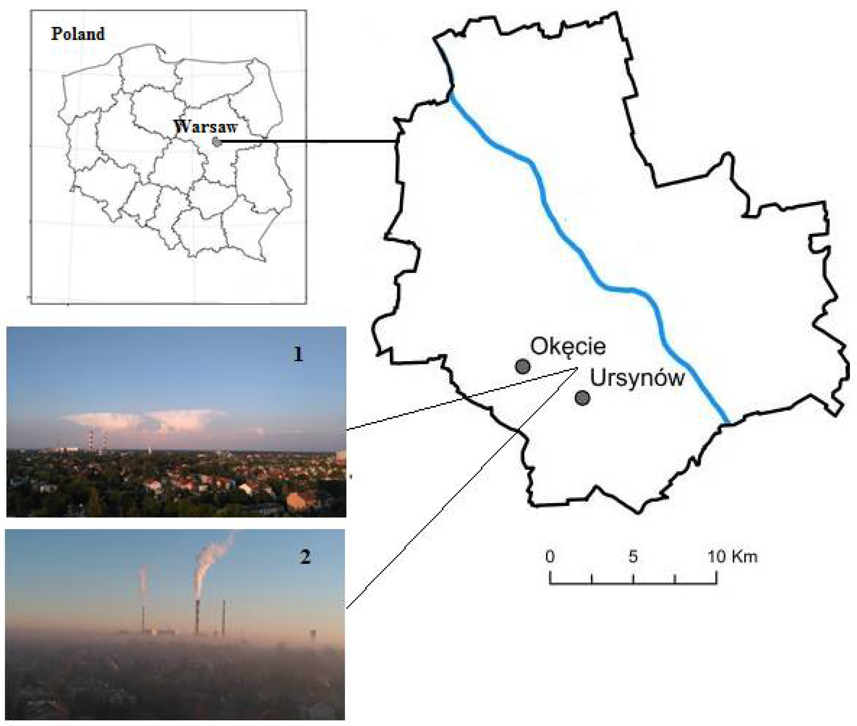
2. Research Object and Employed Device

The paper is based on the measurements carried out in Warsaw, Poland (Figure 1). Warsaw is the largest city in Poland (517.2 km²) located in the temperate climate zone. The climate of this area, due to its location in the central part of Europe, is subject to maritime and continental influences. The measuring station (Warsaw-Ursynów) is located in the southern part of Warsaw (λE = 21°02′, φN = 52°09′). The study used the data on hourly average concentrations of the following air pollutants: SO₂, CO, O₃, NO₂, and PM₁₀, monitored via pulsed fluorescence, infrared absorption, absorption of ultraviolet light, chemiluminescence, and a β -gauge automated particle sampler, respectively. The weather data were taken from the Ursynów-SGGW weather station (λE 21°02′, φN 52°09′). In turn, the visibility data originate from the Warszawa-Okęcie station (λE 20°59′, φN 52°09′). A visibility meter with an atmospheric phenomenon detector—Vaisala FS11 was used to carry out the measurements of visibility. It served as an atmospheric phenomenon detector and a visibility meter using light dispersion measurements. The horizontal visibility was measured in the range of 10 m–50 km. During rainfall events, FS11 measures the beam attenuation due to scattering processes and does not physically account for absorption, e.g., by water vapor. However, the scatterometer response resembles a (visible light band) transmissometer response in the typical range of weather conditions. According to the manufacturer, the response of FS11 has been tested, evaluated and verified 25 times by means of a transmissometer including a visible light band emitter, at different locations around the world. Hence, the absorption effect is accounted for to a certain extent.

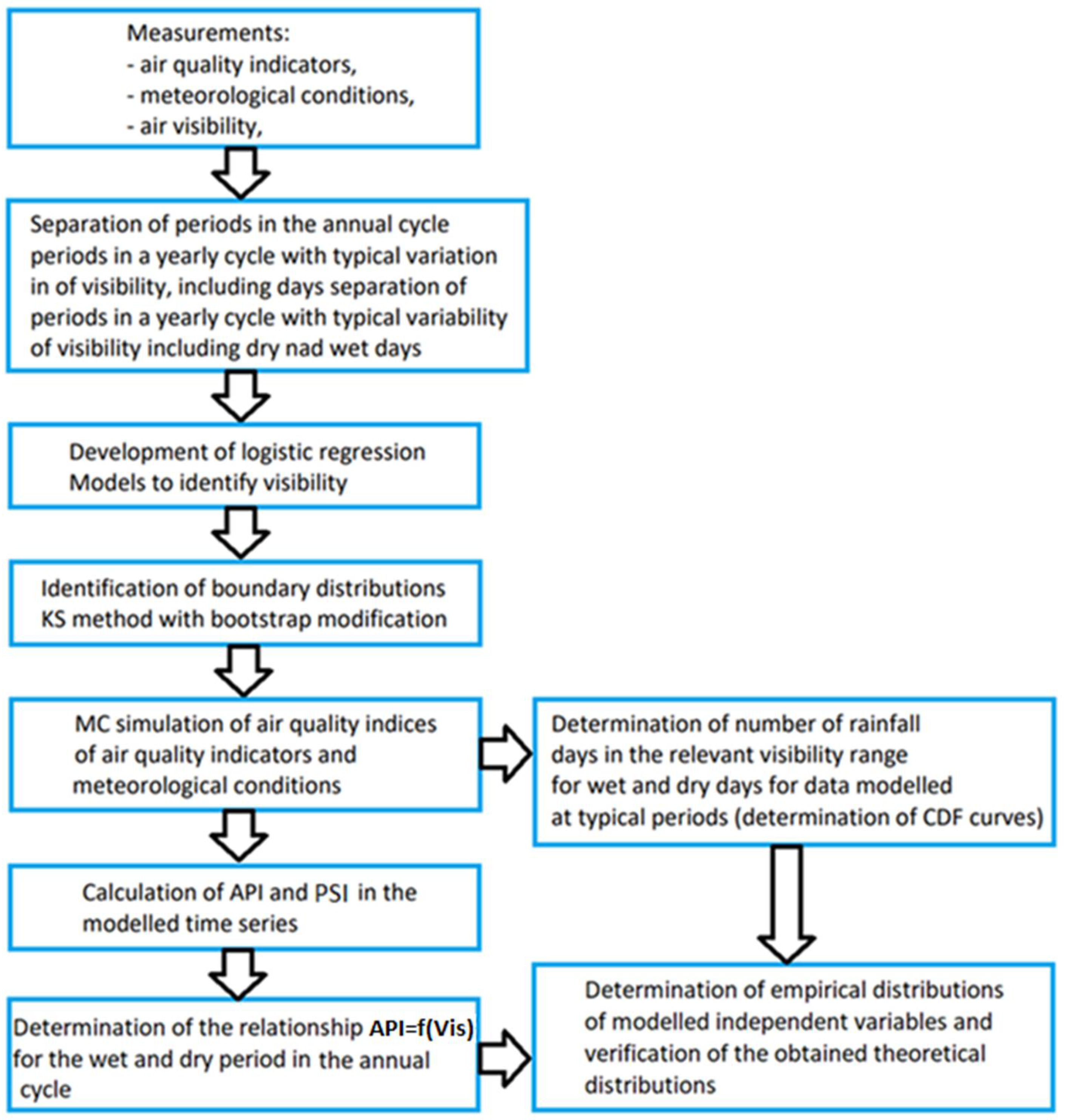
3. Methodology of Data Analysis and Model Creation

A novel computational model has been proposed, the algorithm of which is presented in Figure 2. It enables us to analyze the influence of air visibility as well as weather conditions on the relationship between the Air Pollution Index (API) and values of other chosen air quality indices. The model also allows determining the number of days per month in separate periods of the annual cycle with air visibility in an appropriate range of variability, taking into account the rainfall conditions. The developed model comprises six independent modules. The first one includes input data (air quality, weather conditions) necessary in subsequent modules. In the second module, a cluster analysis is performed, which allows separating the periods of typical visibility variability in the annual cycle, taking into account the rainfall conditions. In the third module, logistic regression models are created to identify visibility in appropriate K ranges of variability. In the fourth module, empirical distributions of separated independent variables of logit models are determined and then theoretical distributions of these variables are fitted (bootstrap variant of the Kolmogorov–Smirnov and chi-square tests with [18]. In the fifth module, using the obtained theoretical distributions, the simulations of monthly series of air quality and the weather conditions, including the rainfall data, are performed for separated typical periods in the annual cycle.

In the sixth module, the number of days in a month with appropriate visibility variation is determined for separated periods of the year for the dry and wet periods. In the seventh module, on the basis of generated data (air quality, weather conditions), calculations of visibility, values of air quality indices for wet and dry periods are performed and the relation between API and air visibility is determined. In the eighth module, the simulation results are verified with the measurement data.

4. API and PSI Calculations

Air Pollution Index (API) was adopted to assess the air quality. It is an index that takes into account the concentration of the main pollutants in the air by considering them in a way that indicates their total effect on an organism [19]. There are many well-known formulas for determining the air quality index, adjusted to the needs of the countries in which they are valid. In Poland, no such dependence has been established, and there is no pan-European formula; therefore, the index proposed by Cairncross [20] was employed. This index is a scale expressing the functional relationship between the following parameters: average daily concentration of sulfur dioxide (SO₂), maximum daily concentration of carbon monoxide (CO), maximum daily concentration of nitrogen dioxide (NO₂), average daily concentration of particulate matter PM₁₀ or PM_2.5 (this paper uses daily measurements for the PM₁₀ fraction), maximum hourly or 8-hourly tropospheric ozone (O₃) concentration per day (this paper uses measurements averaged to 1 h) and risk of short-term negative health effects [20]

In order to build API, relative mortality risk (PR) values for each pollutant were assumed. The total risk of simultaneous short-term exposure for several pollutants is the sum of the concentration values of all pollutants:

(PR − 1)_tot = ∑_i(PR_i − 1)

(1)

where: i = 1, 2, …, 5—number of consecutive pollutants PR_i—relative mortality risk [19].

A set of PR values was used for: PM, SO₂, NO₂ and O₃ published by WHO as part of the procedure for assessing health effects of pollutants in the European Union [21]. A so-called pollutant sub-index (PSI) was also defined to reflect the contribution of individual pollutants to the total risk:

PSI_j = a_j ∙ (exposure index_j)

(2)

where: j—pollutant, a_j—directly proportional to incremental risk values, exposure index—pollutant concentration from a certain combination of averaging.

API is a sum of five pollutant sub-indices:

API = ∑_i PSI_i = ∑_i a_i ∙ C_i

(3)

where: Ci—concentration of the i-th pollutant, a_i—proportionality coefficient for the i-th pollutant [20]. On the basis of [19], the proportionality factor values were assumed for: PM₁₀: a_i = 0.05; for SO₂: a_i = 0.02703; for O₃: a_i = 0.03108; for NO₂: a_i = 0.02027; for CO: a_i = 0.27027.

Ten classes of atmospheric air quality were adopted, with an eleventh class open for the values exceeding PSI_i = 9. PM₁₀ particulate matter was assumed to be the priority pollutant and PSI classes were made depending on this factor. The permissible concentration of PM₁₀ from 24h was taken as the lower limit of the third class. The other classes were calculated proportionally based on Equation (2). With reference to the Cairncross classification [20], the following cut-off points were proposed:

• Low (1–3): low risk for increased mortality: 1.5–6.0%,
• Medium (4–6): medium risk for increased mortality: 6.1–10.6%,
• High (7–9): high risk for increased mortality: 10.7–15.3%,
• Very high (10): very high risk for increased mortality: above 15.3%.

5. AQI and API Calculations

A hierarchical cluster analysis method was used to separate typical visibility periods in the annual cycle taking into account wet and dry days [22]. Cluster analysis is a set of methods used to separate homogeneous subsets. On the basis of the variables that characterize the objects under analysis, cluster analysis finds groups (clusters) of objects that are similar to each other and shows how similar one cluster is to others or, which is often more important, how strongly it differs from other clusters and objects in them. The end result of this process is usually a dendrogram, or hierarchical clustering tree, which allows for an easy and clear graphical representation of the results obtained from the analyses. On dendrograms, a specific distance measure is used to express the proximity of analyzed objects. The objects with high similarity are separated by a small distance and naturally merge into larger clusters, while a large distance separates strongly dissimilar objects. There are many distance measures, defined in different ways, an overview of which can be found in the paper [23,24,25]. The most popular measure, called Euclidean distance, was used in this study. In order to determine the distance between formed clusters of objects, Ward’s method was applied, which determines the smallest possible variance in separated clusters [26,27].

On the basis of the results of measurements (the 2004–2013 period) of meteorological conditions (T—temperature, Rh—relative humidity, w—velocity of wind, P—rainfall depth) and air quality indices (SO₂, NO_x, O₃, CO, PM), a dendrogram was created to determine the number of typical periods (N) per year taking into account the rainfall conditions. These analyses also focused on accounting for seasonality in the annual cycle [22].

6. Logistic Regression

Logistic regression (binomial logit model) can be used as a classification tool. Its advantage over other methods (regression trees, neural networks, support vectors, etc.) consists in that it enables probability modeling; therefore, the results of logit calculations are continuous values in the range of 0–1. On the basis of the literature review [28,29] it can be concluded that the logit model finds applications in social, economic, natural and technical sciences. Logistic regression (for splitting the measurement data of the dependent variable into two groups) can be used for visibility simulation and assumes the following form:

$$\mathrm{p}=\frac{\exp \left({{\displaystyle \sum }}_{\mathrm{i}=1}^{\mathrm{M}}{\mathsf{\alpha }}_{\mathrm{i}}·{\mathrm{x}}_{\mathrm{i}}+{\mathsf{\alpha }}_0\right)}{1+\exp \left({{\displaystyle \sum }}_{\mathrm{i}=1}^{\mathrm{M}}{\mathsf{\alpha }}_{\mathrm{i}}·{\mathrm{x}}_{\mathrm{i}}+{\mathsf{\alpha }}_0\right)}$$

(4)

where: p—probability of exceeding the Vi_sm visibility value, x_i—independent variables, i.e., air quality indices (SO₂, NO_x, O₃, CO, PM, etc.), weather conditions (temperature, relative humidity, wind speed, rainfall), season.

The analyses performed by Majewski et al. [22] using HCA (Hierarchical Cluster Analysis) for the analyzed visibility measurement point, weather conditions, and air quality indicated that the year can be divided into three periods—clusters, in which the above-mentioned factors are similar. The results of calculations performed by Majewski et al. [22] showed that rainfall depth is the factor that affects the variation of visibility values in the obtained clusters.

According to the literature [22], in the calculations, it is assumed that a value of p ≥ 0.5 corresponds to values of Vis > Vis_m. In turn, when p < 0.5, then the Vis values obtained from Equation (4) are smaller than Vis_m. Sensitivity (SENS), specificity (SPEC) and counting error (Rz2) are used to evaluate the agreement between the results of calculations and measurements in the logit model. At the model development stage, the correlation of independent variables was analyzed, VIF values were determined and the variables for which it was greater than 5 were rejected [22]. In the analyzed model, the forward stepwise method—preferred for the logistic regression method—was used to identify coefficients (α_i) and thus the independent variables statistically significant at the assumed confidence level.

This paper proposes the possibility of using logistic regression to model simultaneously K-classes (more than two) of variation in air visibility values. In this solution, the key is to determine the (K-1) limiting the visibility values Vis_j constituting the basis for dividing the measurement data into binary values. In this study, seven visibility limits ranging from Vis₁ = 8 km to Vis₇ = 24 km with a step of ΔVis = 4 km were adopted for analysis. This approach was intended to thoroughly analyze the influence of measurement data (weather conditions, air quality) on air visibility and to identify the mechanisms involved, which are determined by the factors mentioned above. For K = 7 visibility values (Vis₁, Vis₂, Vis₃, Vis₄, Vis₅, Vis₆, Vis₇) underlying the classification of Vis measurement results, consecutive logit models can be given:

$$\mathrm{p}\left(\mathrm{Vis}>{\mathrm{Vis}}_{\mathrm{j}}\right)=\frac{\exp \left({{\displaystyle \sum }}_{\mathrm{i}=1}^{\mathrm{M}}{\mathsf{\alpha }}_{\mathrm{i},\mathrm{j}}·{\mathrm{x}}_{\mathrm{i},\mathrm{j}}+{\mathsf{\alpha }}_{0,\mathrm{j}}\right)}{1+\exp \left({{\displaystyle \sum }}_{\mathrm{i}=1}^{\mathrm{M}}{\mathsf{\alpha }}_{\mathrm{i},\mathrm{j}}·{\mathrm{x}}_{\mathrm{i},\mathrm{j}}+{\mathsf{\alpha }}_{0,\mathrm{j}}\right)}\mathrm{for}\mathrm{j}=1,2,\dots ,7$$

(5)

For Equation (5), the following ranges of visibility variation were separated:

${\langle \mathrm{Vis}}_{\min },{\mathrm{Vis}}_1)$, ${\langle \mathrm{Vis}}_1,{\mathrm{Vis}}_2)$, ${\langle \mathrm{Vis}}_2,{\mathrm{Vis}}_3)$, ${\langle \mathrm{Vis}}_3,{\mathrm{Vis}}_4)$, ${\langle \mathrm{Vis}}_4,{\mathrm{Vis}}_5)$, ${\langle \mathrm{Vis}}_5,{\mathrm{Vis}}_6)$, ${\langle \mathrm{Vis}}_6,{\mathrm{Vis}}_7)$, ${\langle \mathrm{Vis}}_7,{\mathrm{Vis}}_{\max }\rangle$, determined based on the measurement data.

7. Identification of Marginal Distributions

This procedure was carried out on the basis of the data from measurements conducted at a daily resolution, involving air quality and weather conditions [30]. At first, the measurement data were divided into two periods—wet and dry. Within the two periods, the data from winter (I, II, XI, XII), transitional (III, IV, IX, X) and summer (V, VI, VII, VIII) periods were separated, for which the average visibility values were 10.5 km, 17.0 km and 22 km respectively [22]. On the basis of the estimated logit models, the empirical distributions of the independent variables (x_i) of these models were determined. In the next step, theoretical distributions were fitted to the empirical distributions. For this purpose, five distributions (parametric) were used: log normal, Frechet, Gumbel, Weibull and Gamma [31]. The consistency of empirical and theoretical distributions was assessed based on the bootstrap variant of Kolmogorov–Smirnov and chi-square tests [18].

8. Simulation of Air Quality Indices and Weather Conditions Using the Monte Carlo Method

A modified Monte Carlo–Iman Conover (MC-IC) method was used to simulate the time series of air quality indices and weather conditions. In this solution, the correlation between the analyzed independent variables in the logistic regression model is taken into account. In the simulation procedure, the theoretical distributions of the analyzed independent variables in the logit models, for separated periods in the annual cycle, were taken as the boundary distributions. The simulations covered a period of one month for typically separated periods in an annual cycle, which resulted from the specificity of measurement data—the resolution of measurements amounted to one day. A detailed description of MC-IC simulations and limitations is presented in Iman Conover [32] and Majewski et al. [22].

9. API Relationship Considering the Visibility and Rainfall Data

Determination of the number of days when the visibility varies within the appropriate range was performed according to the following steps:

-

Simulation (10,000 samples) of air quality indices and weather conditions for Pk wet days (for a single month) using the Iman Conover method from theoretical distributions in the winter, transition and summer period.

-

Simulation (10,000 samples) of air quality indices and weather conditions for (30-Pk) dry days (for a single month) using the Iman Conover method from theoretical distributions in the winter, transition and summer period.

-

Calculation of probabilities of exceeding the Vis_i visibility values in separated classes (Equation (5)) for wet days in the winter, transition and summer period.

-

Calculation of probabilities of exceeding Vis_i visibility values in separated classes (Equation (5)) for dry days in the winter, transition and summer period.

-

Estimation of the number of days (for 10,000 samples) with visibility values in the appropriate range of variability (Equation (5)) for wet days in the winter (15 days), transition (16 days) and summer (18 days) period in a single month.

-

Estimation of the number of days (for 10,000 samples) with a visibility value within the appropriate range of variability (Equation (5)) for dry days during the winter (15 days), transition (14 days) and summer (12 days) period in a single month.

-

API calculations (for 10,000 samples) for wet days with a visibility value in the relevant range of variability (Equation (3)) in the winter, transition and summer period; for the analyzed range of variability Vis, calculations of API values are performed when the data obtained from simulations with the I-C method meet one of the conditions given in Equation (3).

-

Calculation of API (for 10,000 samples) for dry days with visibility value in the relevant range of variability in the winter, transition and summer period.

-

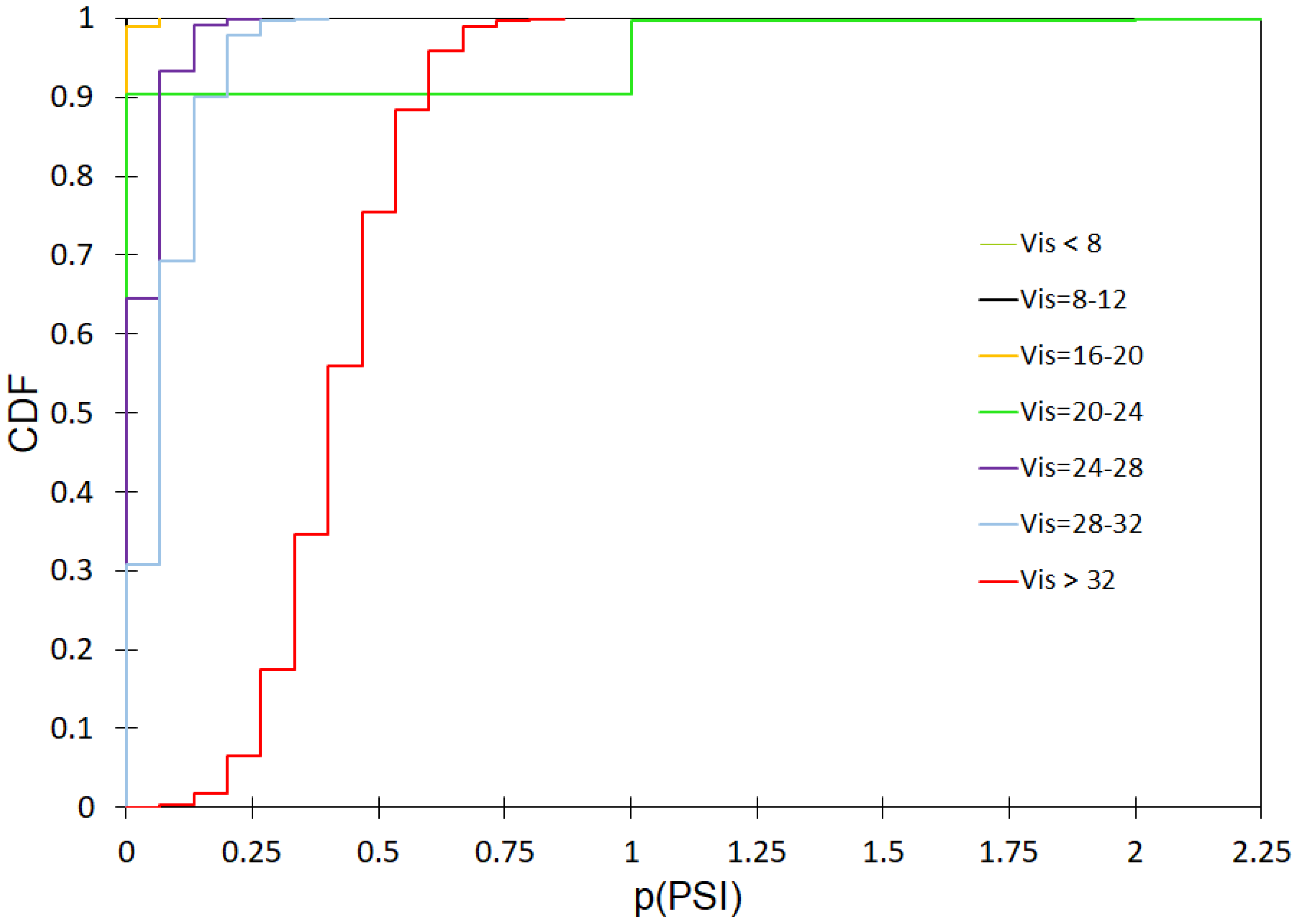
Determination of empirical distributions (CDF) describing the probability of exceeding the number of days with visibility in separated classes (Equation (5)) for wet and dry weather for the winter, transitional and summer period.

-

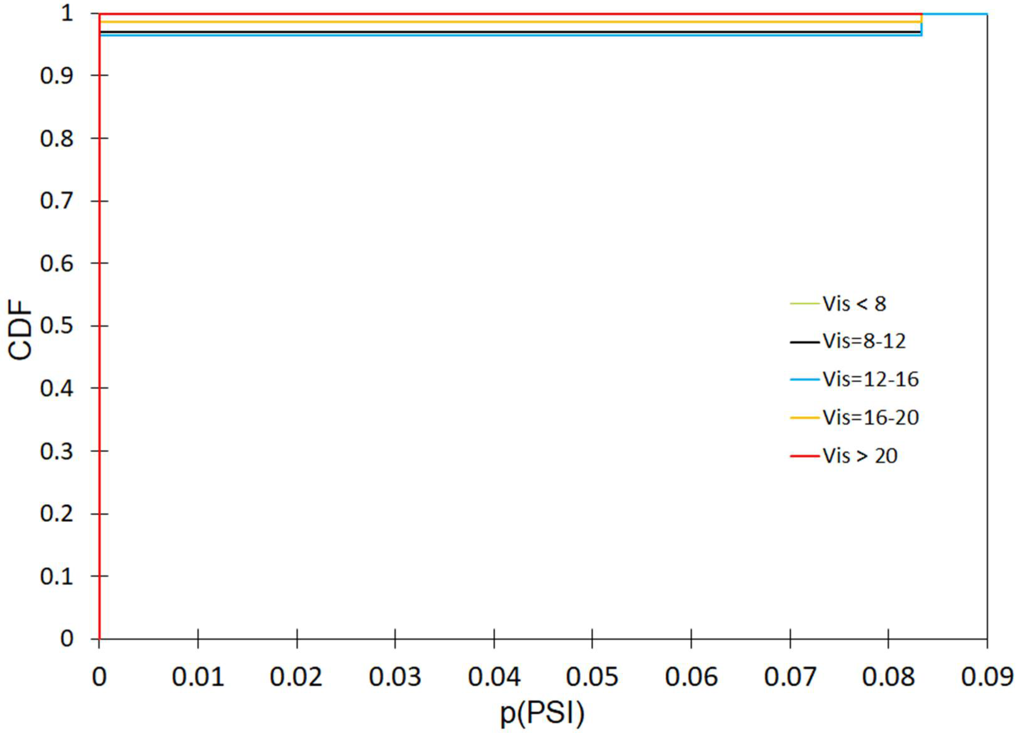
Determination of empirical distributions (CDF) describing the probability of exceeding API of days for visibility values in separated classes (Equation (5)) for wet and dry weather for the winter, transitional and summer period.

The simulation results of the number of days per month with the corresponding visibility range in the annual cycle are verified by comparing the theoretical distributions with the empirical distributions obtained from the measured data. API simulation results (theoretical distributions) obtained for the analyzed periods in the annual cycle for wet and dry days are verified in an identical way.

10. Results

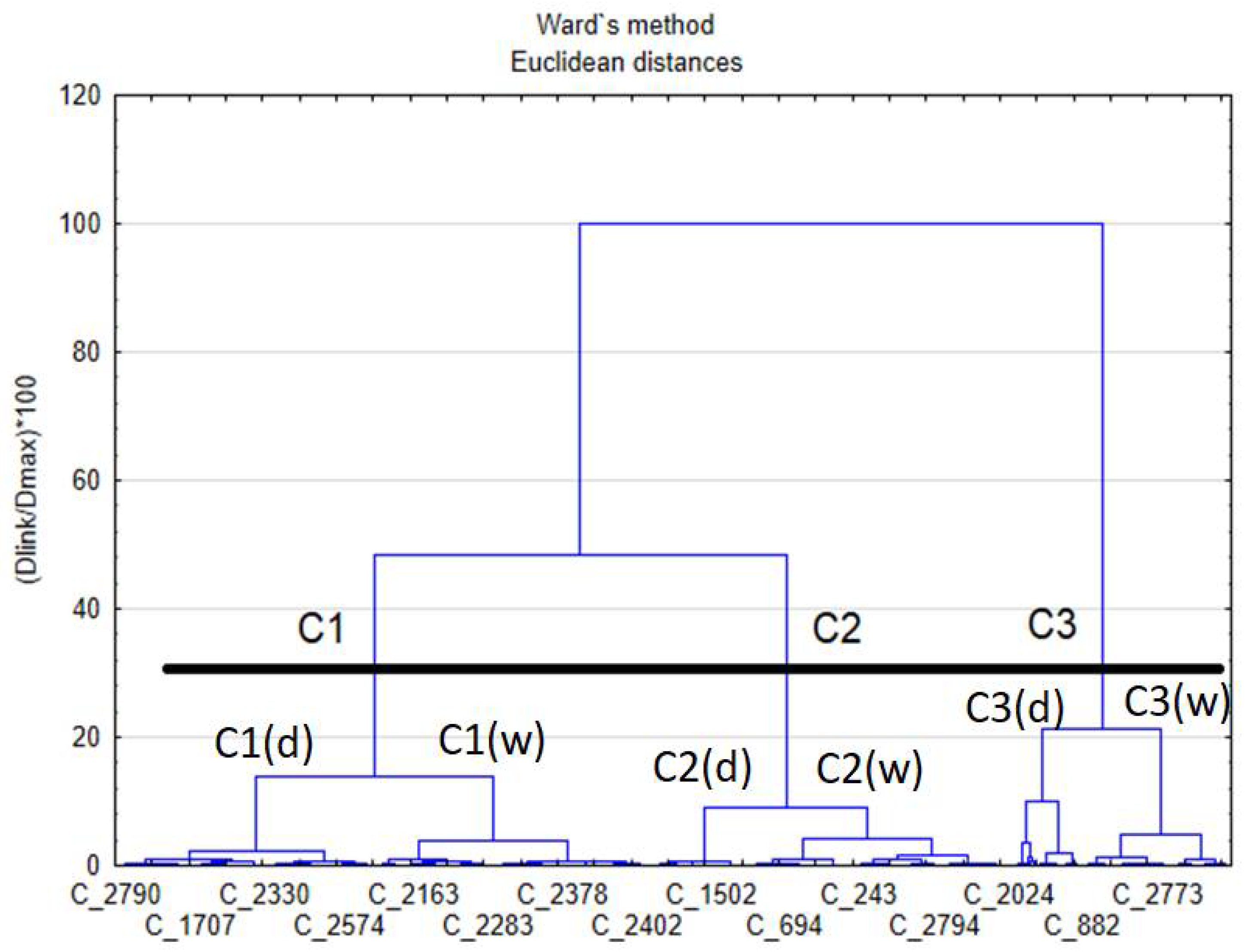
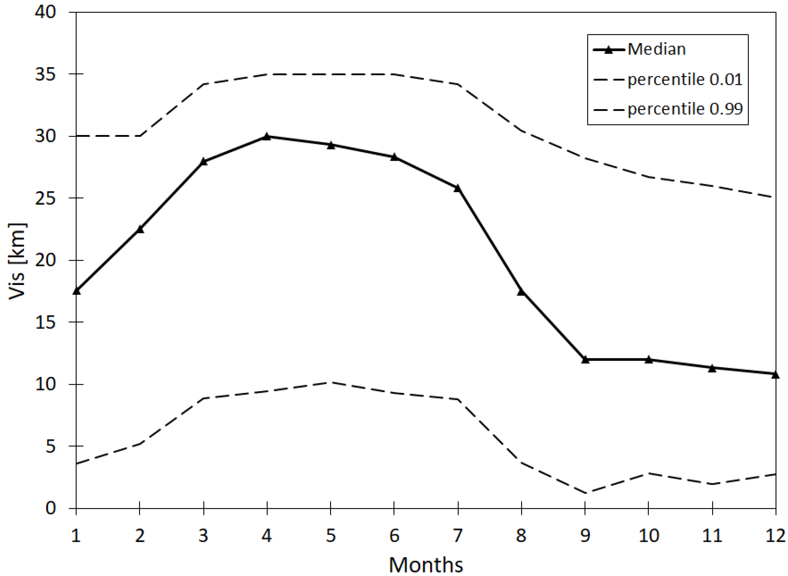
10.1. Separation of Typical Periods in the Annual Cycle

On the basis of the results obtained from measurements of weather conditions and air quality, a dendrogram was created using the cluster analysis method (Figure 3). In these calculations, a single linkage method and the data clustering method, i.e., Ward’s method, was adopted. The performed calculations (Figure 3) showed that the year can be divided into three typical periods of visibility variability [22]. These data fall into the following periods: I, II, XI, XII and III, IV, IX, X and V, VI, VII, VIII. These periods reflect the seasonality in the annual cycle in the corresponding clusters. The following mean temperature values were obtained: 3.5 °C for C1, 10.6 °C for C2 and 18.5 °C for C3. On the basis of the calculations performed, it was found that two more clusters could be separated in each cluster. The data analysis showed that lower values of the analyzed air quality indices were obtained in each of the clusters C1(d), C2(d), C3(d) compared with C1(w), C2(w), C3(w) and they correspond to the wet days. This is confirmed by the data related to the rainfall depth in the separated clusters. The results of calculations obtained using cluster analysis are confirmed by the results of variability analysis (mean, 0.01 and 0.99 percentiles) in relation to consecutive months in the annual cycle (Figure 4).

During periods I, II, XI, XII, the average visibility is 11.54 km, while for III, IV, IX, X, it is equal to 20.84 km, and during periods V, VI, VII, VIII, it averages 28.83 km.

10.2. Separation of Typical Periods in the Annual Cycle

Using the forward stepwise algorithm for model creation and eliminating variables for which VIF > 5, logistic regression models were developed for the following threshold values Vis = 8, 12, 16, 20, 24, 28, 32 km, after the considered independent variables underwent Cox–Box transformation properly. The results of calculating the test probability (p) for the analyzed air quality indices and weather conditions are given in

Table 1. Results of test probability (p) calculations for selected independent variables and fit of calculation results to the measurements performed in logistic regression models.

Variables	Visibility [km]
	8	12	16	20	24	28	32
	p
PM10	0.0011	0.0010	0.0034	0.0123	0.0078	0.0111	0.0126
SO2	0.0160	0.0253	0.1360	0.0546	0.3450	0.4210	0.3560
CO	0.0210	0.0321	0.2670	0.0782	0.0128	0.1530	0.0236
NO2	0.0300	0.0276	0.3190	0.1230	0.0245	0.0287	0.0219
O3	0.2510	0.0317	0.4650	0.0342	0.0289	0.0353	0.0345
T	0.0016	0.0211	0.0120	0.0216	0.0110	0.0267	0.0129
V	0.0235	0.0541	0.0267	0.0432	0.2340	0.3460	0.0238
Rh	0.0124	0.0121	0.0231	0.0187	0.0120	0.0098	0.0111
Pt	0.0156	0.0349	0.0365	0.0401	0.0312	0.0278	0.0421
Pe(z)	0.0234	0.1230	0.0342	0.0423	0.0345	0.0327	0.2780
Pe(l)	0.0341	0.0980	0.0289	0.0383	0.0156	0.0278	0.3260
DP	0.2310	0.7890	0.5430	0.4890	0.4670	0.0345	0.0341
SENS	92.2	95.2	97.7	96.5	97.4	96.2	93.2
SPEC	93.3	96.4	94.2	94.3	95.3	94.1	91.8
Accuracy	93.0	96.0	96.5	95.7	96.3	95.6	92.7

. Moreover, the values of the obtained measures of fit between the calculation results and measurements, i.e., SENS, SPEC and Accuracy, are presented. The values of the determined coefficients in the logistic regression models are given in

Table A1. Results of computing α_i coefficients in logit models.

Variables	Coefficients
	Vis = 8	Vis = 12	Vis = 16	Vis = 20	Vis = 24	Vis = 28	Vis = 32
PM10	−0.121	−0.124	−0.127	−0.116	−0.086	−0.086	−0.096
SO2	0.000	0.000	0.000	0.061	0.000	0.000	0.029
CO	0.000	0.000	0.000	0.000	0.002	0.002	0.002
NO2	0.000	−0.014	−0.016	−0.014	0.000	0.000	−0.033
O3	−0.008	−0.014	−0.016	−0.021	0.000	0.000	0.008
T	0.109	0.119	0.109	0.106	0.086	0.086	0.128
w	0.082	0.000	0.000	0.109	0.216	0.216	0.000
Rh	−0.191	−0.204	−0.195	−0.177	−0.239	−0.239	−0.226
Pt	−0.049	−0.069	−0.073	−0.168	−0.004	−0.004	−0.030
Pe(z)	0.239	0.585	0.459	0.000	1.349	1.349	0.000
Pe(l)	0.417	0.299	0.134	0.000	−0.423	−0.423	0.000
Intercept	17.984	18.716	17.543	14.311	23.997	23.997	22.145
DP	0.000	0.000	−0.324	−0.351	−0.086

. The obtained calculation results (Table 1) confirm the differential influence of weather conditions and air quality indices on the air visibility values. This is proven by the test probability values, which show that for Vis > 16 km, the SO₂ values have no statistically significant effect on the modeled Vis probability values.

In contrast, no statistically significant effect of NO₂ was shown for Vis = 16–20 km. For the O₃ values, no statistically significant effect was shown for Vis = 8 km and Vis = 16 km, whereas in the case of the V values—for Vis = 12 km and Vis = 24–28 km. Table 1 also indicates a good fit between the calculation results and measurements, as confirmed by the SENS, SPEC and Accuracy values varying in the ranges 92.2–97.7%, 91.8–96.4% and 92.7–96.5%, respectively. This shows that the obtained models provide a useful tool for visibility modeling for the considered measurement post. The obtained calculation results confirm the complex relationship between visibility and the air quality indices as well as weather conditions included in the analyses [33,34]. This may indicate that transformations of pollutants in the air depending on weather and air quality conditions shape the variability of visibility in the air. This is confirmed by the calculated values of α_i coefficients in logistic regression models, which are highly variable depending on Vis values. The finding obtained in the present analyses (introduction of multiple classes of visibility changes) has not been analyzed so far in visibility simulation models [35], which may explain why it was so difficult to obtain high agreement between calculation results and measurements. For example, for Vis < 8 km, the values of PM₁₀, SO₂, NO₂, and CO do not affect the air visibility. For Vis = 12–16 km, among the considered air quality indices, visibility is affected by PM₁₀, NO₂ and O₃. For Vis > 28 km, air visibility is affected by PM₁₀, SO₂, NO₂, CO, O₃, while for Vis > 32 km, Vis is only affected by the PM₁₀ values. Despite the complex nonlinear relationships between air visibility and air quality as well as weather conditions, some typical relationships were shown. The obtained analytical results confirm the calculations of So et al. [36], who demonstrated the influence of temperature, humidity and selected air quality indices on visibility using the example of southwestern British Columbia. The relationships reported in the paper are also confirmed by the calculations performed by Majewski et al. [17], who developed a model to forecast air visibility using the linear regression method while obtaining the R² values < 0.65. The calculation results reported in the paper are also confirmed by Lee et al. [37], who analyzed the data for Southeast Asia and showed a strong influence of quality indices on visibility for selected cities (Hanoi, Singapore, Manila and Badung). Strongly nonlinear relationships between visibility and air quality indices which cannot be captured by linear regression models were demonstrated by Pan et al. [37], who showed visibility forecast errors of 0.5–8.09% using SVM and ANN modified with genetic and ant swarm algorithms.

10.3. Determination of Empirical and Theoretical Models

Using the bootstrap variant of the Kolmogorov–Smirnov test [38], the parameters of the theoretical distributions for air quality indices were determined for three typical periods of the year, i.e., I, II, XI, XII and III, IV, IX, X and V, VI, VII, VIII. The results of calculating the test probability (p) and the obtained parameters of the distributions are given in

Table A2. Best fit theoretical distributions (according to Kolmogorov–Smirnov test) for the variables.

Variable xi	Distribution	Parameters	p (K-S)
(I) period: Nov.–Feb.
PM10	lognorm	μ = 3.503 σ = 0.611	0.489
SO2	lognorm	μ = 2.326 σ = 0.541	0.612
CO	lognorm	μ = 6.315 σ = 0.403	0.745
NO2	gamma	μ = 25.744 k = 5.004 β = 4.922	0.225
O3	Weibull	μ = 0.211 β = 1.854 γ = 32.231	0.115
T	Weibull	μ = −77.42 β = 17.42 γ = 80.149	0.625
Rh	GEV	k = −0.014 β = 1.159 μ = 1.749	0.415
(II) period: Mar.–Apr. and Sep.–Oct.
PM10	Lognorm	μ = 3.462 σ = 0.492	0.951
SO2	Lognorm	μ = 1.963 σ = 0.527	0.924
CO	Lognorm	μ = 6.112 σ = 0.398	0.625
NO2	Lognorm	μ = 3.007 σ = 0.441	0.215
O3	GEV	k = 0.237 β = 20.164 μ = 40.020	0.416
T	Weibull	β = 5.921 γ = 31.941 μ = 20.478	0.321
Rh	Weibull	k = 12.053 β = 150.112 μ = −72.321	0.474
(III) period: May–Aug.
PM10	lognorm	μ = 3.207 σ = 0.343	0.865
SO2	GEV	k = −0.072 β = 1.666 μ = 4.307	0.406
CO	GEV	k = 0.06 β = 80.513 μ = 282.12	0.381
NO2	lognorm	μ = 2.902 σ = 0.402	0.911
O3	GEV	k = 0.177 β = 14.372 μ = 54.021	0.633
T	Weibull	β = 2.145 γ = 2.224 μ = 0.318	0.972
Rh	normal	μ = 66.52 σ = 0.102	0.846
P	lognorm	μ = 4.006 σ = 0.734	0.242

. The obtained values of test probability (p > 0.05) confirm the good fit between the theoretical and empirical distributions, which allows us to model their stochastic character using Monte Carlo generators. For this purpose, a modified MC method, i.e., Iman Cover, was used, in which the correlation of independent variables is taken into account at the sampling stage. The analyses performed by Majewski et al. [22] showed that the values of coefficients between the analyzed air quality indices and weather conditions are not larger than R = 0.40. The calculations performed in this study showed that in winter, most of the analyzed air quality indices (PM₁₀, SO₂, CO) can be described by log-normal distributions, whereas NO₂ as well as O₃ by gamma and Weibull distributions, respectively. Variability of temperature (T) and humidity (Rh) can be described by Weibull and GEV distributions. In the spring period, air quality indices (PM₁₀, SO₂, CO, NO₂) can be described by log-normal distributions, while in the case of the O₃ values—by GEV distributions. Variability of weather conditions (T, Rh) is described by Weibull distributions. In summer, variability of the PM₁₀ and NO₂ values is described by log-normal distributions, whereas SO₂, CO and O₃—by GEV distributions. The variability of air temperature and humidity during the period in question is described by Weibull and normal distributions, respectively.

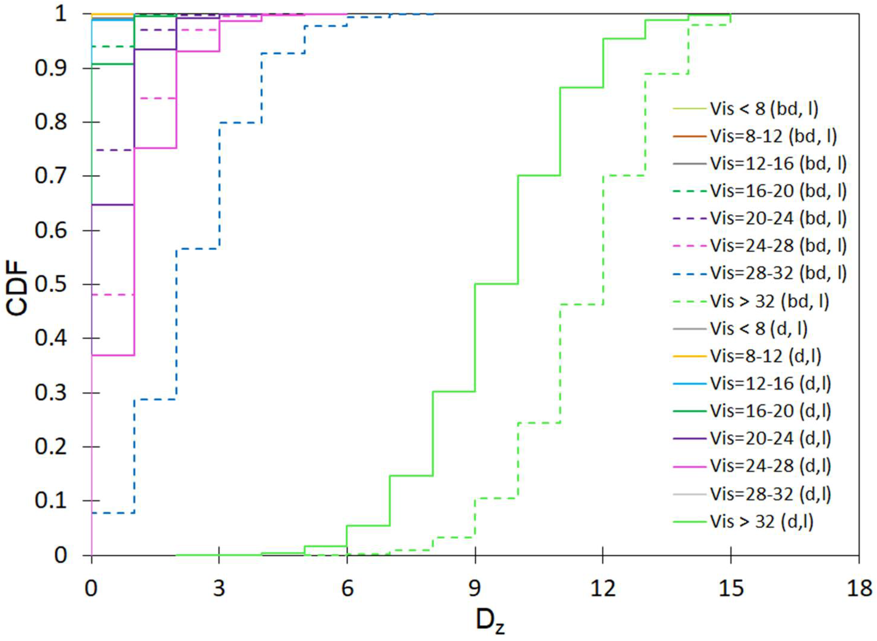
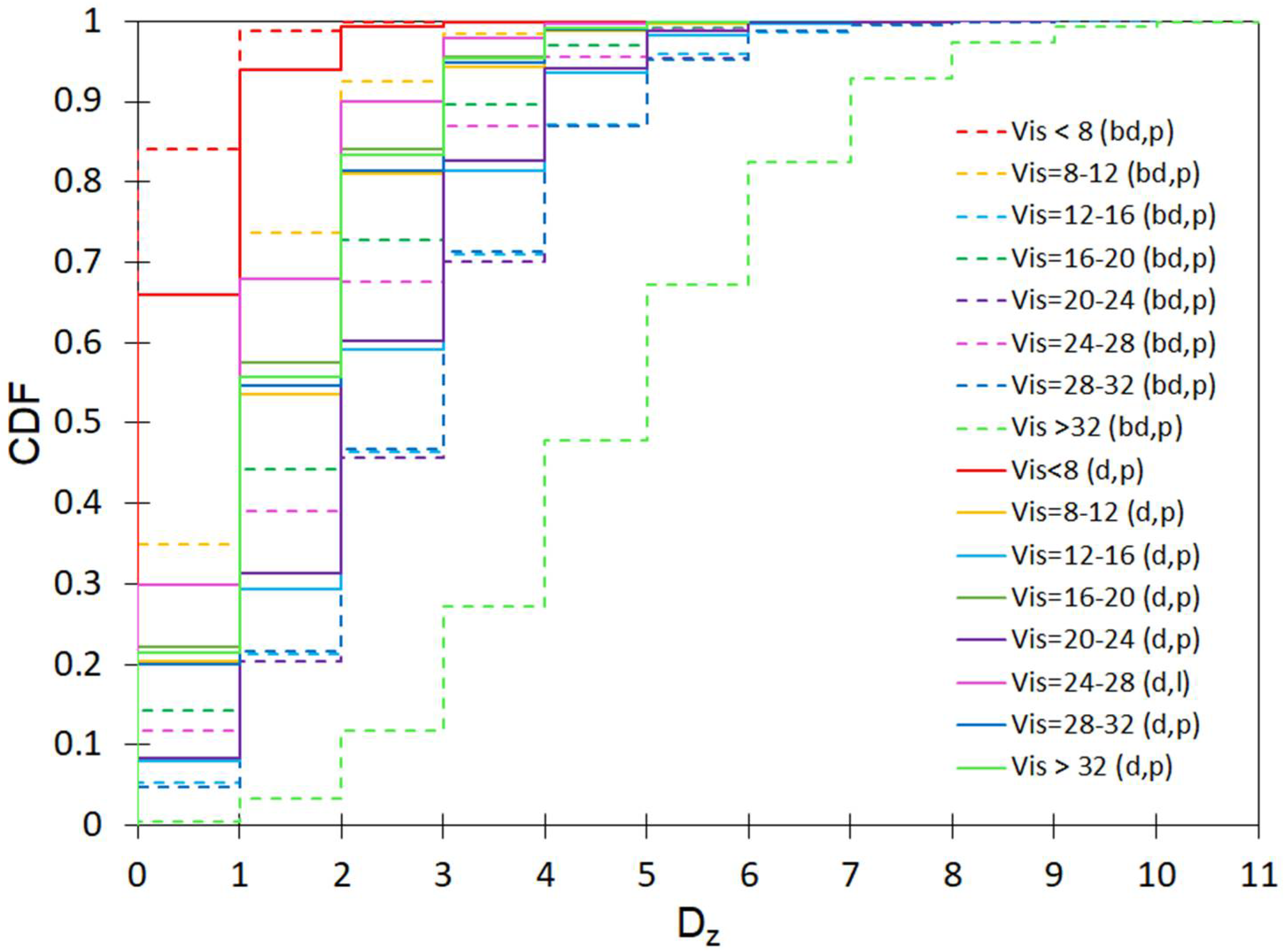
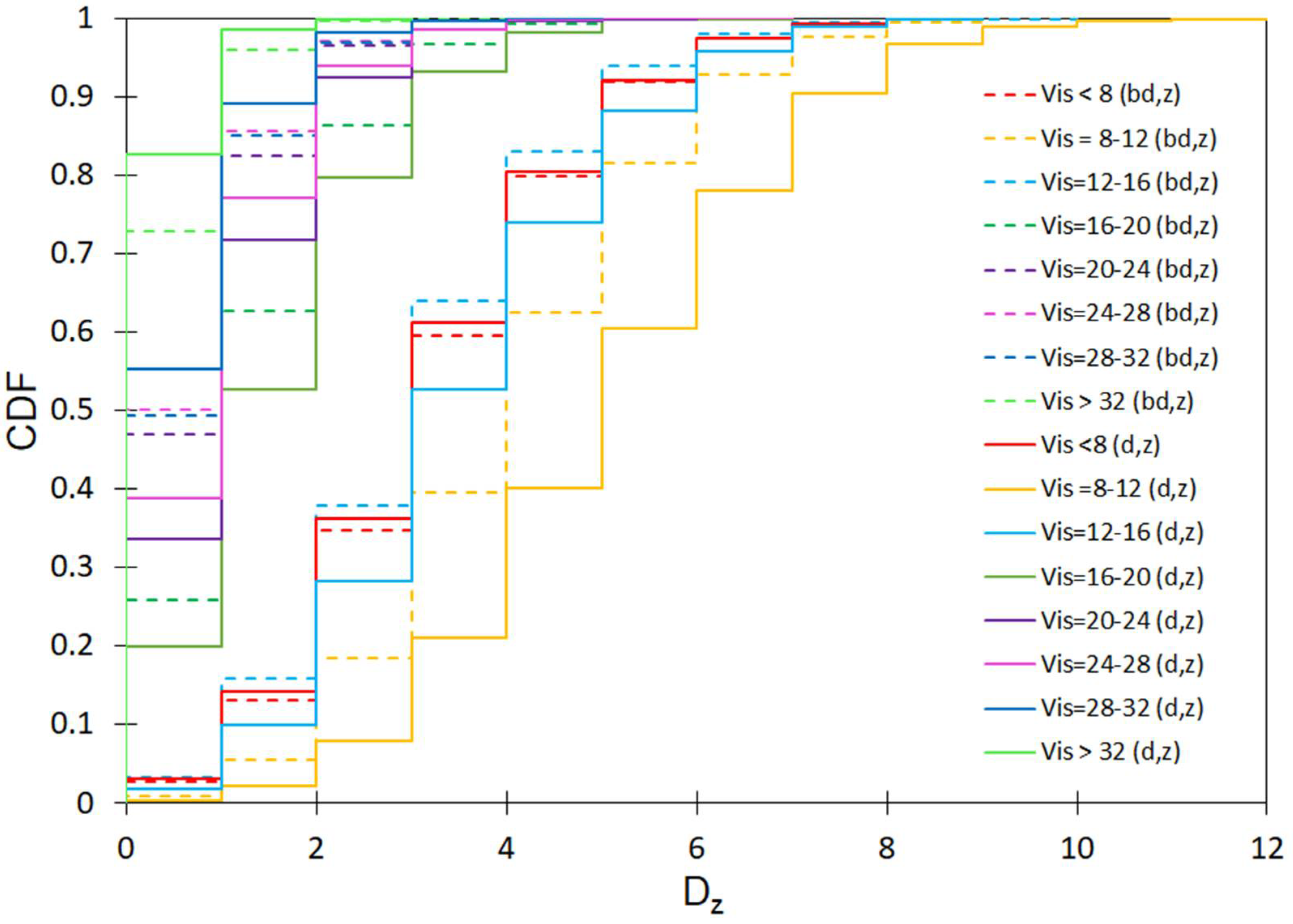
10.4. Calculation of the Number of Days with Visibility in the Assumed Period for Wet and Dry Days

In accordance with the methodology described in Section 9, calculations were performed for the number of days with visibility in the appropriate range in the designated periods: winter (I, II, XI, XII), spring (III, IV, IX, X) and summer (V, VI, VII, VIII) for wet and dry weather. On the basis of the simulations, dependencies were determined, showing the probability of exceeding the number of days in the respective visibility range.

The results of calculations for the considered simulation cases are given in Figure A1, Figure A2 and Figure A3 in Appendix A, while the comparison of the computational results (50%, 95% percentiles) of the number of days with visibility Vis = 8–32 km for wet and dry conditions for spring, summer, and winter were shown in Figure 5a–c. The results of the K-S test calculations showed a good fit between the empirical and theoretical distributions obtained, as confirmed by the test probability values above 0.05 (

Table A3. Results of K-S calculations (probability p) showing the agreement of empirical and theoretical distributions describing the number of days with visibility in the appropriate range for precipitation and rain days for spring, summer and winter seasons.

Visibility	Spring Period		Summer Period		Winter Period
	Wet	Dry	Wet	Dry	Wet	Dry
Vis < 8	0.2046	0.4597	0.3203	0.2427	0.5269	0.4270
Vis = 8–12	0.2089	0.3771	0.5233	0.3361	0.2393	0.2708
Vis = 12–16	0.2989	0.4951	0.4639	0.5245	0.4363	0.6095
Vis = 16–20	0.1512	0.3101	0.3307	0.6060	0.3382	0.4557
Vis = 20–24	0.3525	0.5228	0.0933	0.6296	0.4995	0.1078
Vis = 24–28	0.5082	0.1041	0.2030	0.2690	0.5768	0.4916
Vis = 28–32	0.6401	0.0846	0.4932	0.2388	0.4179	0.2758
Vis > 32	0.3776	0.4473	0.0991	0.5276	0.5013	0.1222

in Appendix A).

On the basis of the calculations performed, it was found that over a period of 12 days for the spring season (wet period) when Vis > 32 km and Vis = 8–12 km amount to 3 days each, for Vis = 12–16 km equals 4 days and 1 day when Vis = 16–20 km, Vis = 20–24 km, Vis = 24–28 km and Vis = 28–32 km. For the dry period in the spring season, over the period of 18 days it was shown that Vis >32 km for 5 days, Vis = 8–12 km for 4 days as well as Vis = 16–20 km, Vis = 20–24 km, Vis = 24–28 km and Vis = 28–32 km for single days. During the summer period for the wet season (15 days per month), Vis > 32 km for 9 days, Vis = 28–32 km for 4 days and Vis = 24–28 km for a single day were shown. For the wet season (15 days per month), Vis > 32 km was found for 11 days, Vis = 28–32 km for 2 days and Vis = 24–28 km for a single day. The calculations for the winter season (wet period, i.e., 16 days in a month) showed that over a two-week period, Vis = 8–12 km for 5 days, Vis < 8 km and Vis = 12–16 km for 3 days as well as 1 day for Vis = 16–20 km, Vis = 20–24 km, Vis = 24–28 km and Vis = 28–32 km. For the dry period (two weeks), it was found that 3 days were shown for a period of 14 days when Vis > 8 km and Vis = 12–16 km, 4 days when Vis = 8–12 km and 1 day when Vis = 16–20 km, Vis = 20–24 km, Vis = 24–28 km and Vis = 28–32 km.

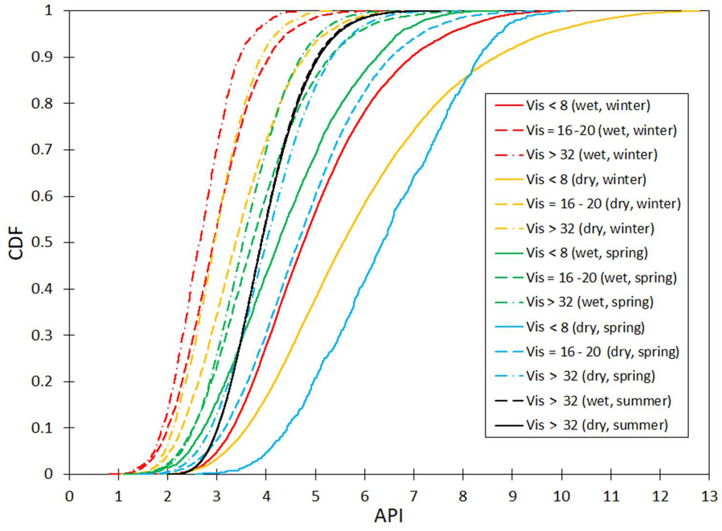
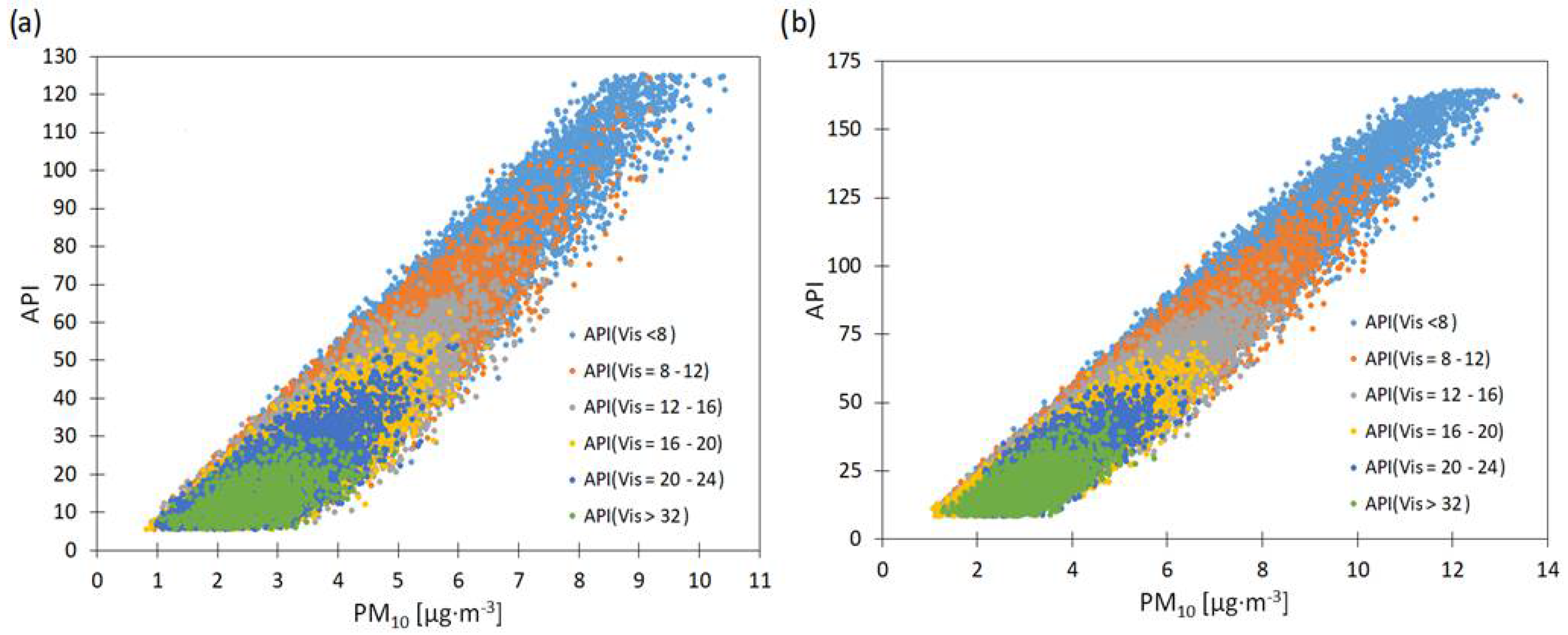
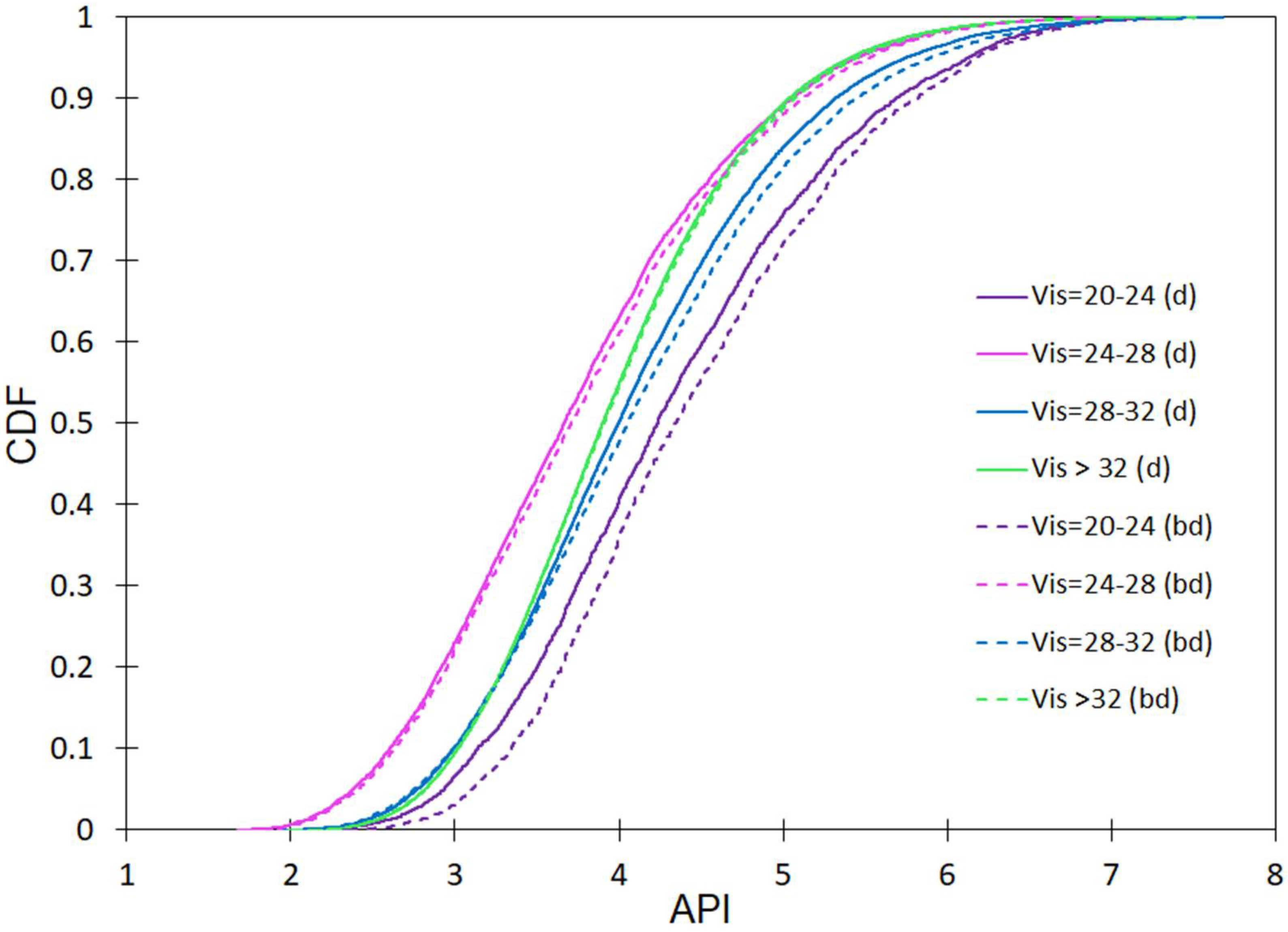
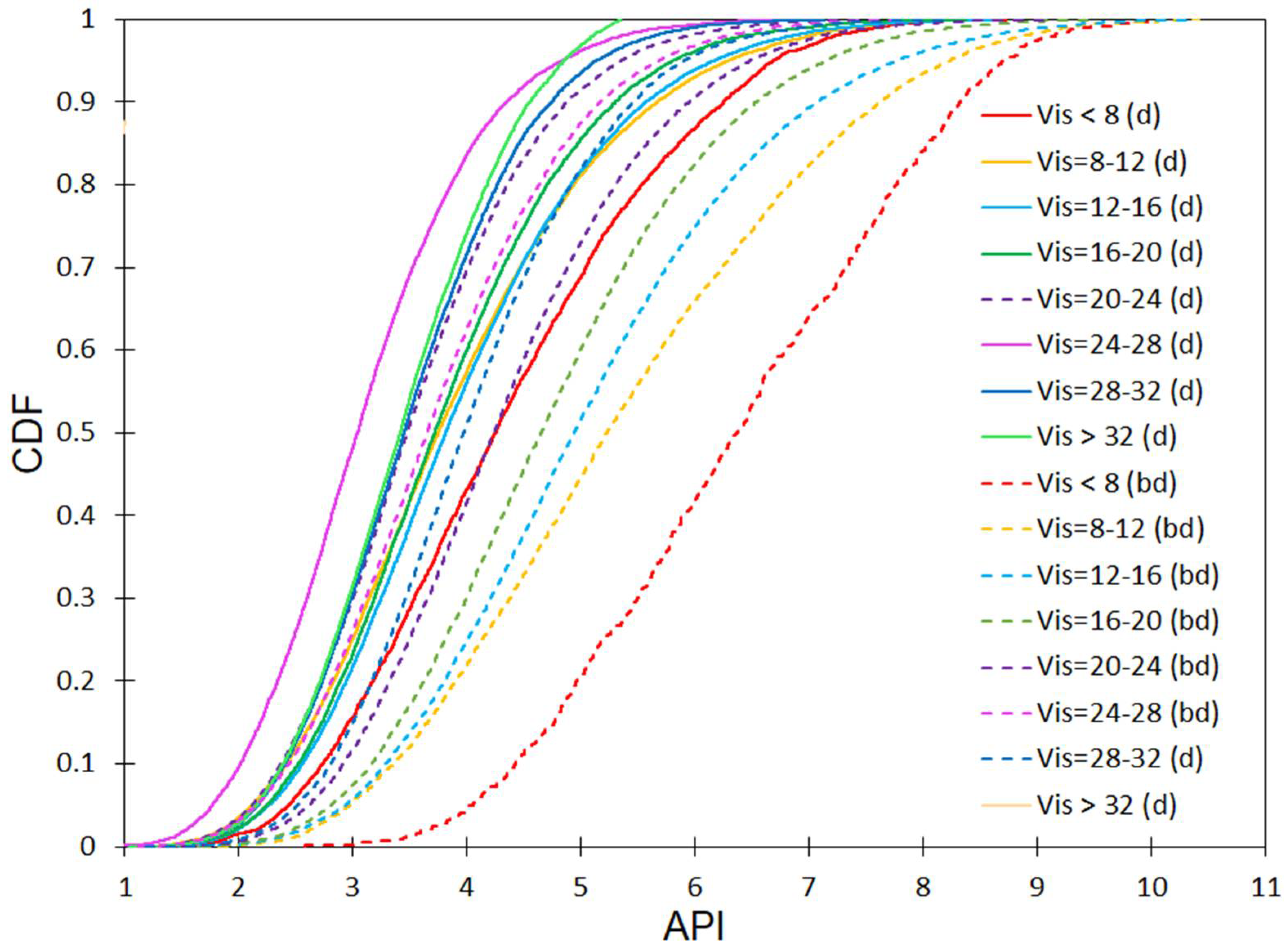
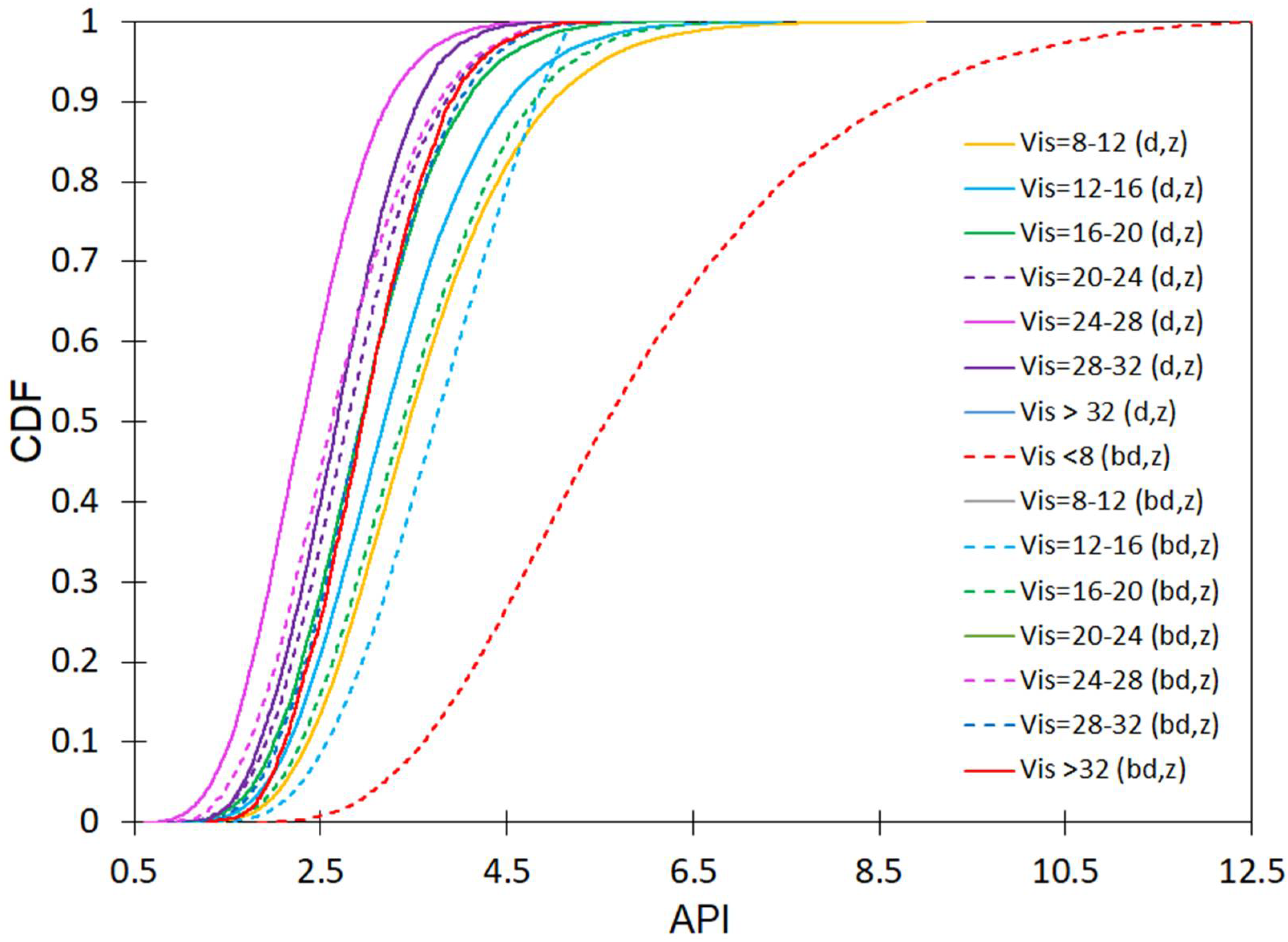
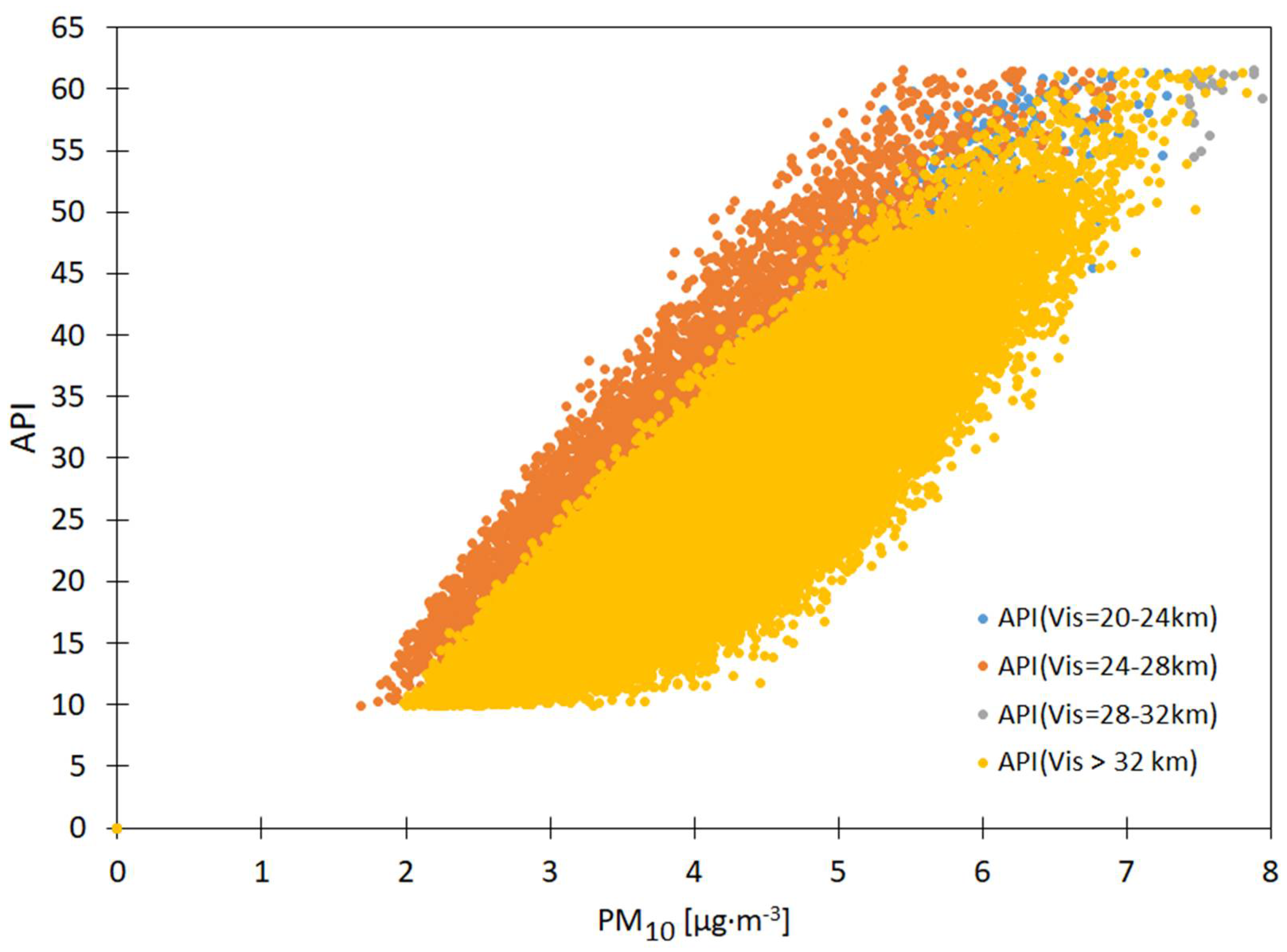
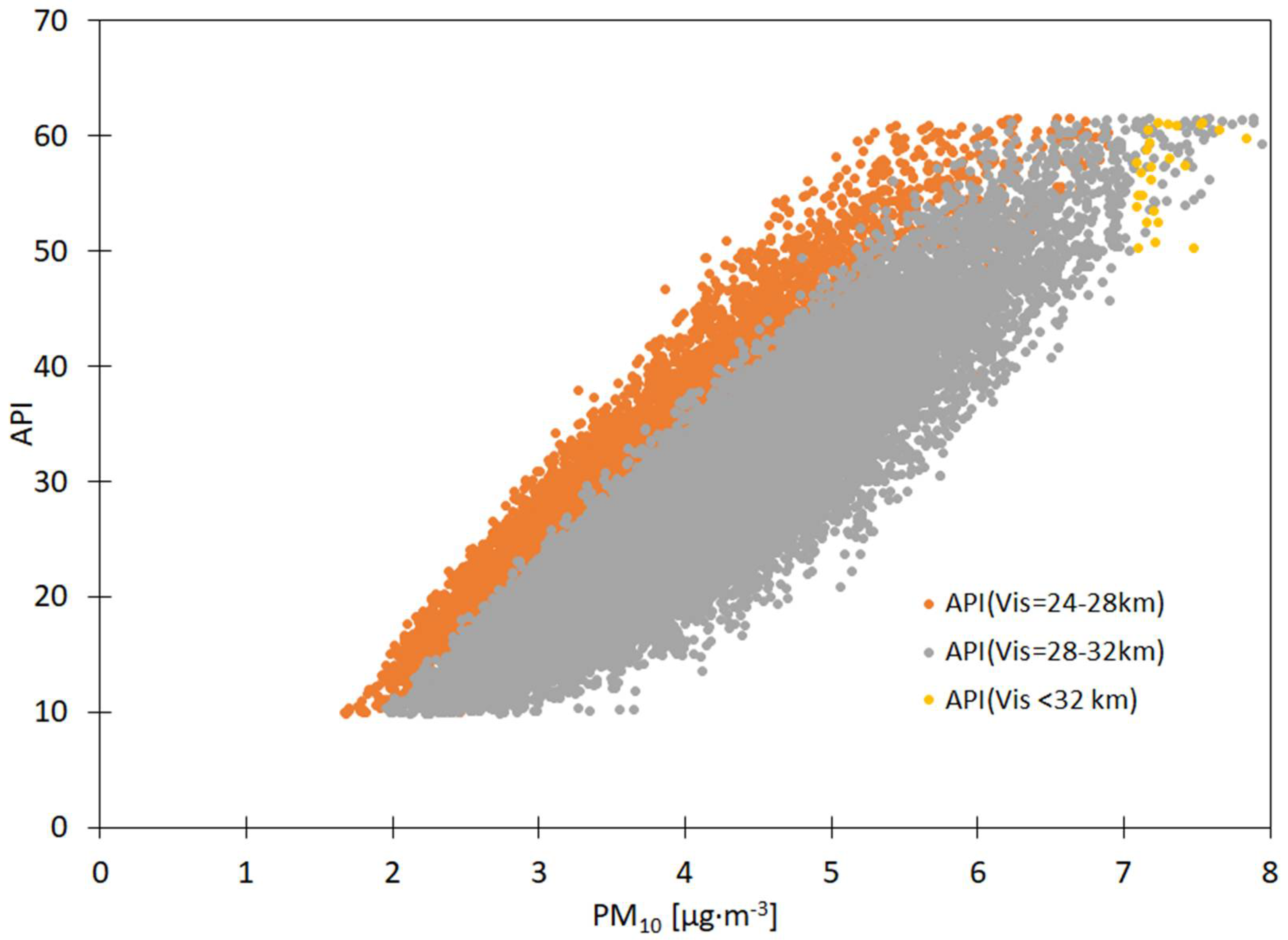
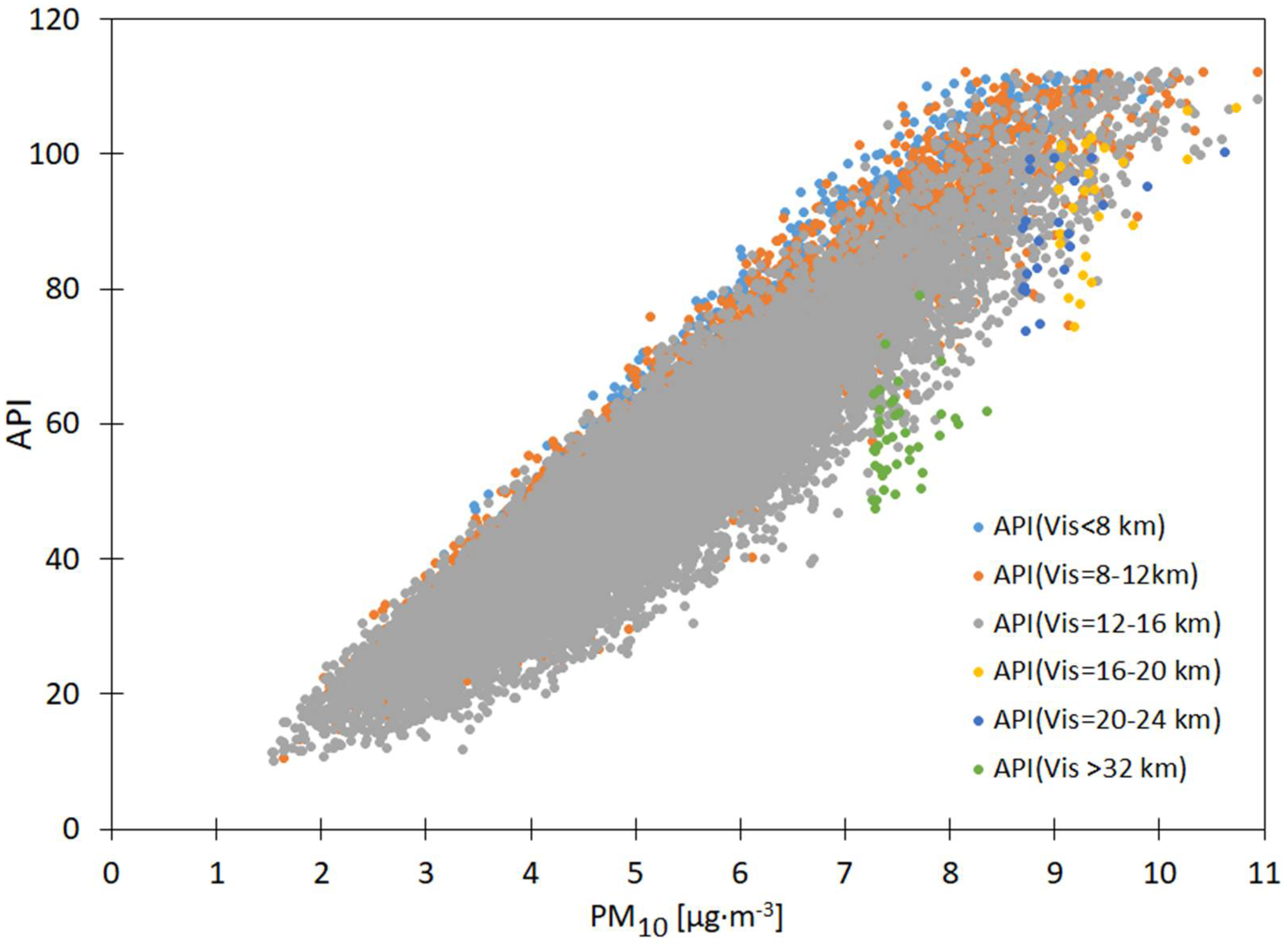
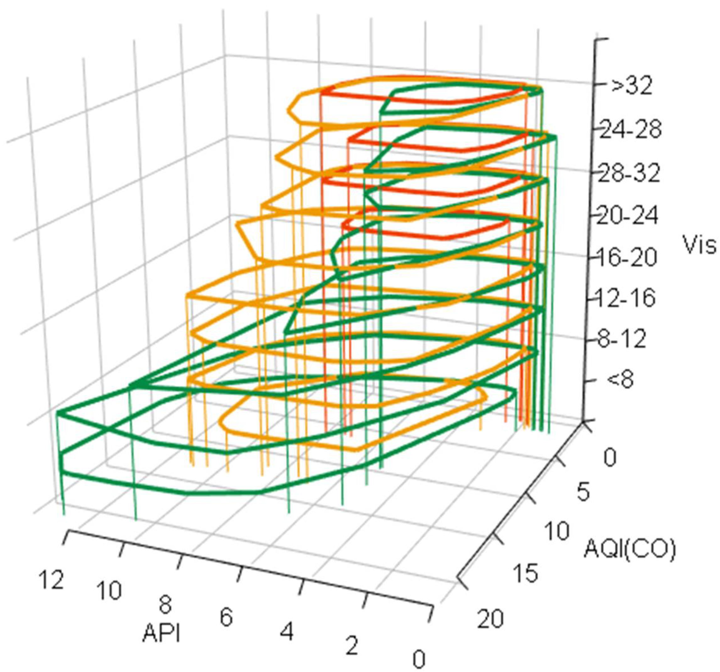
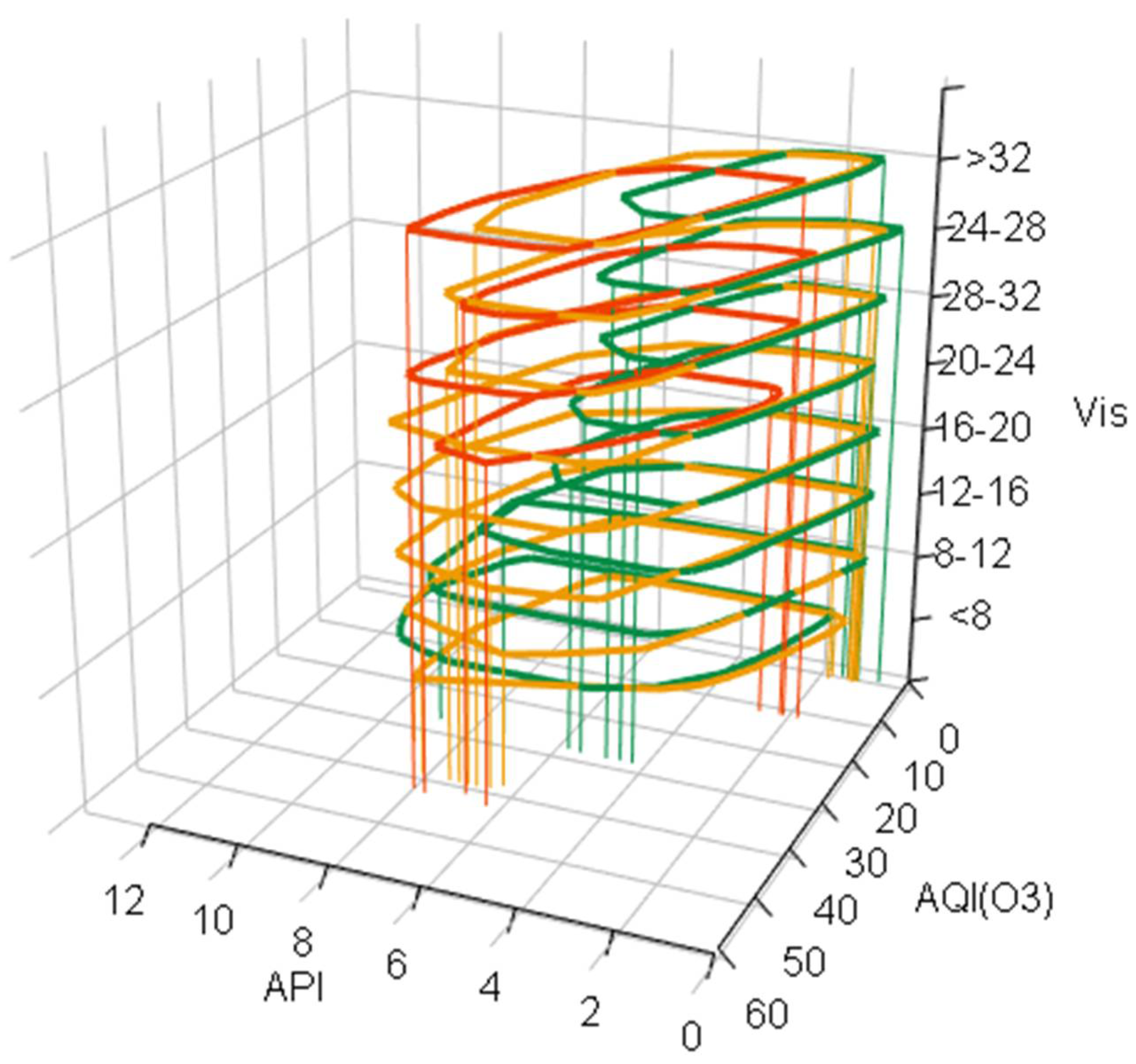
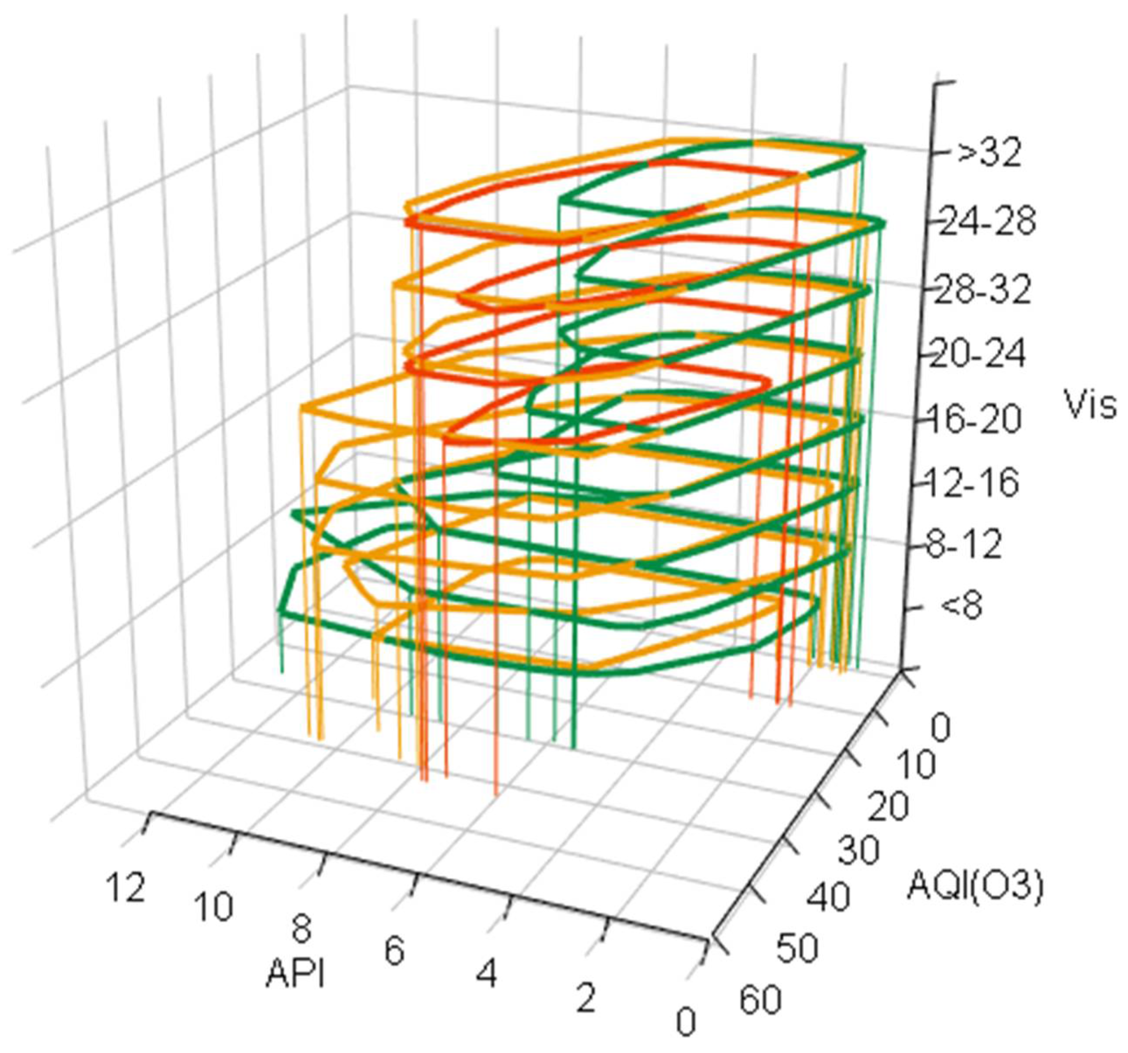
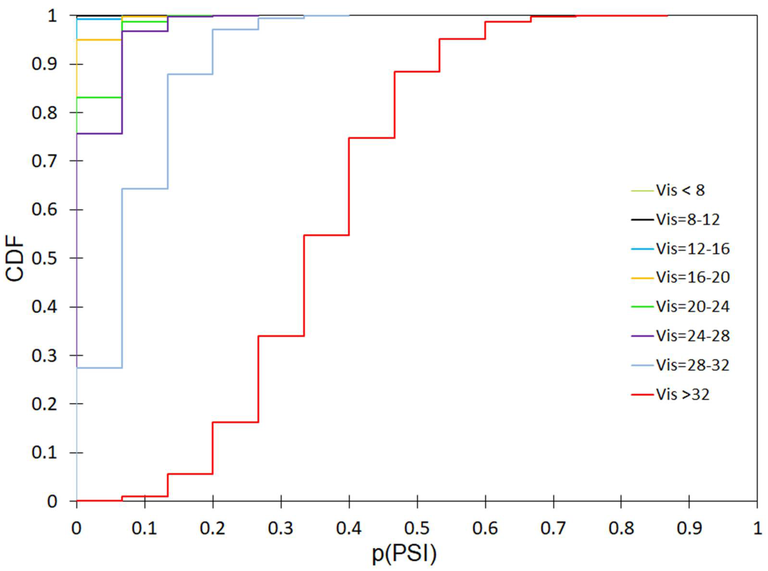
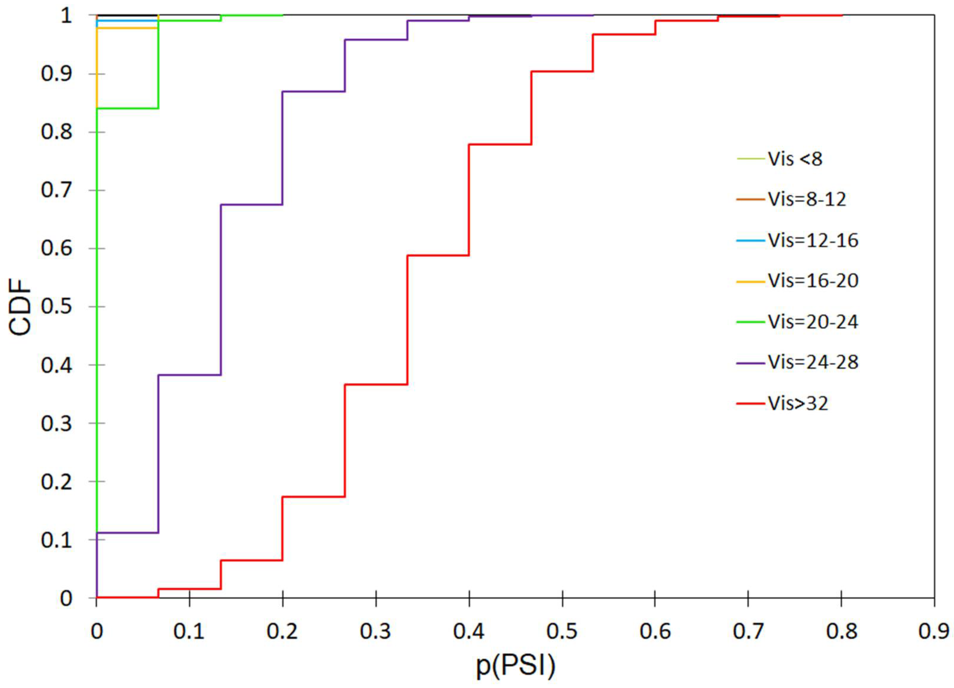
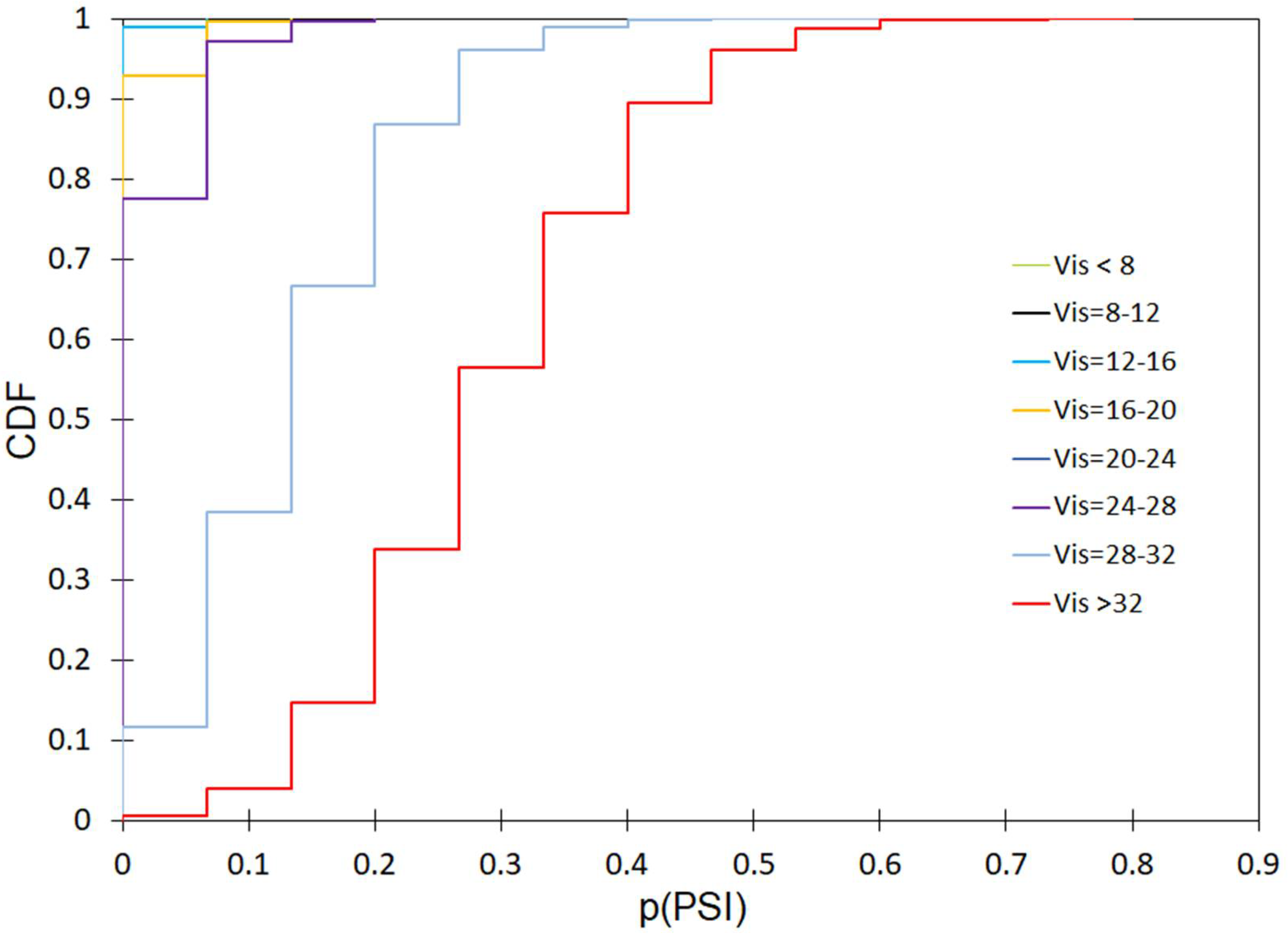
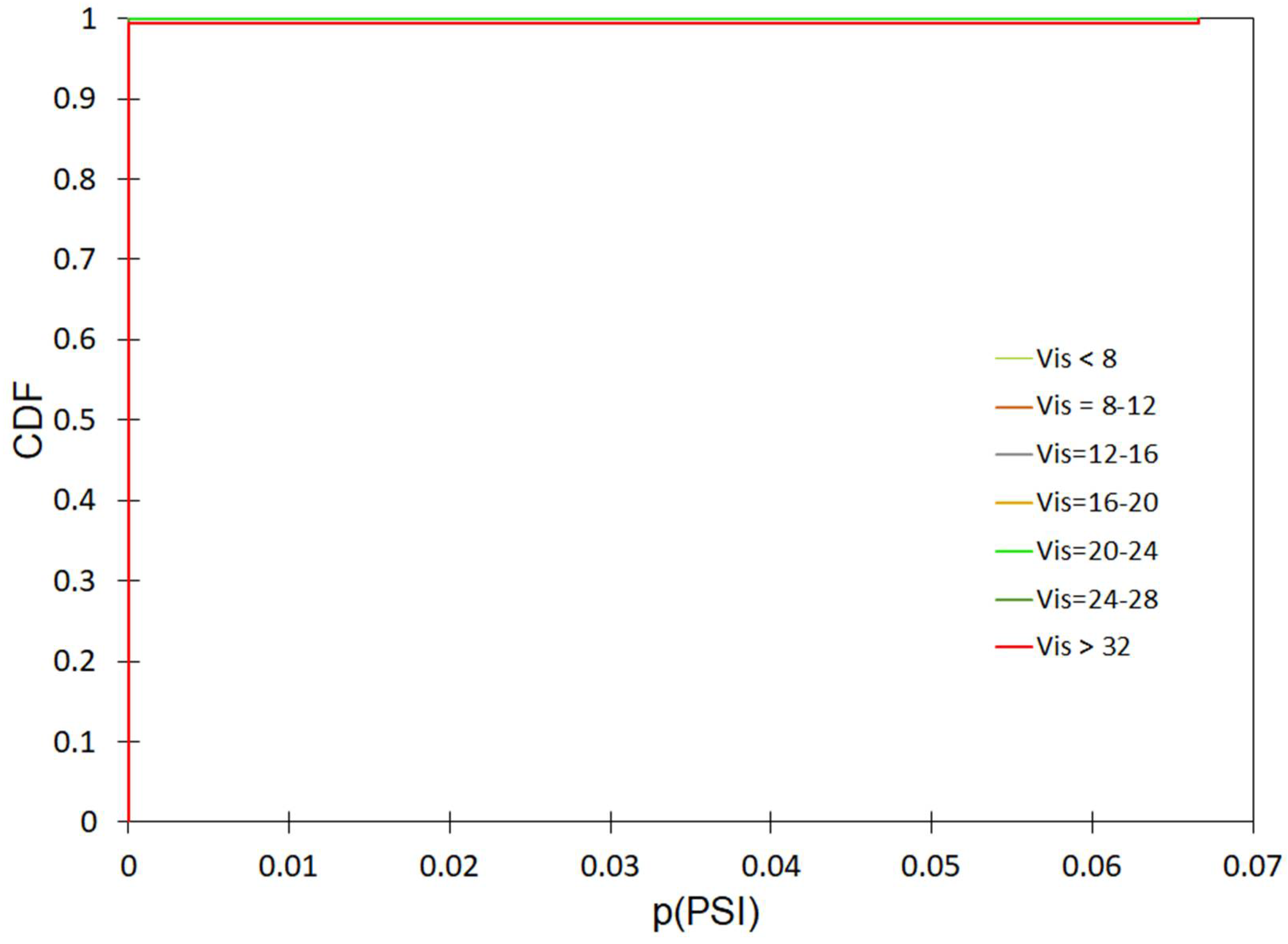
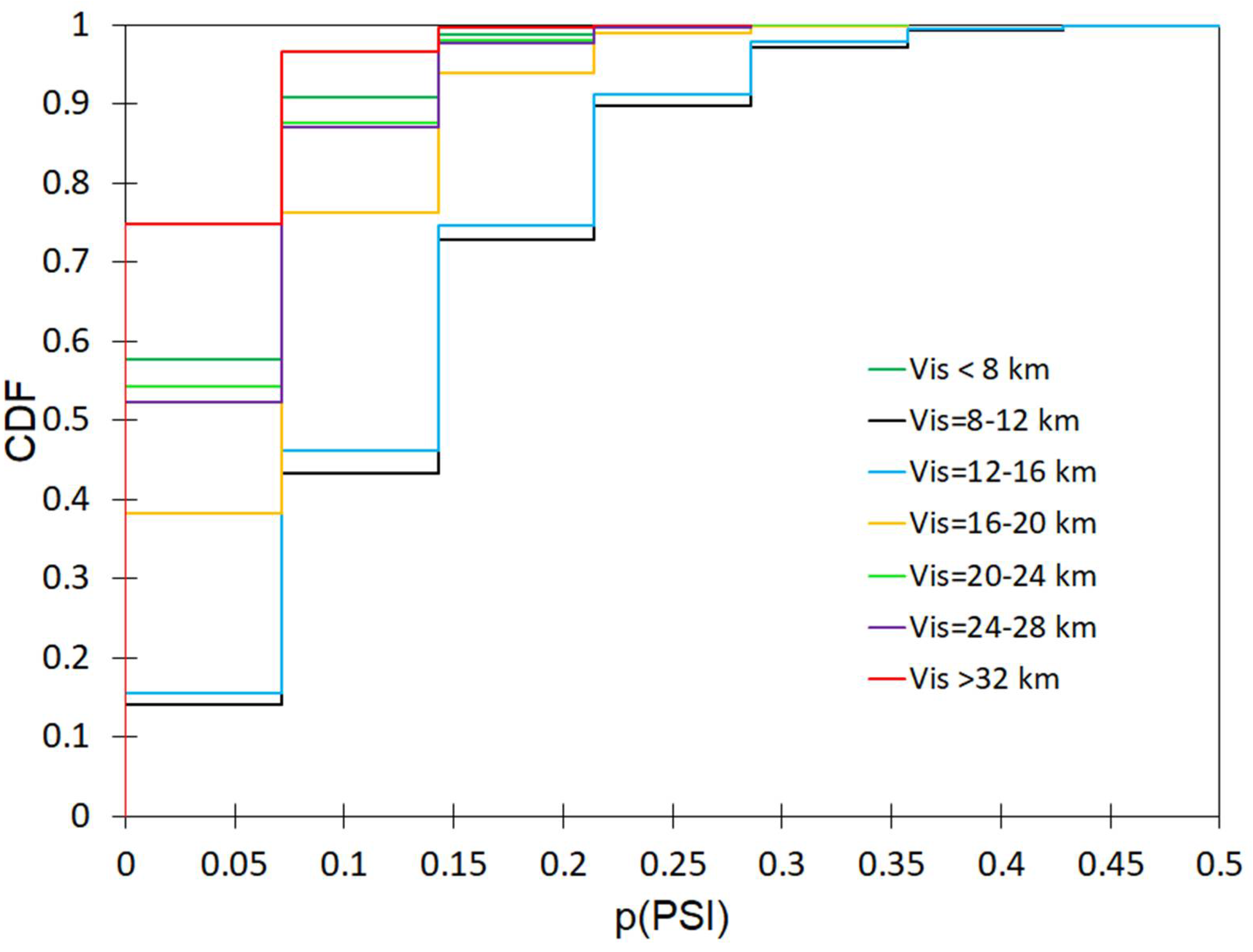
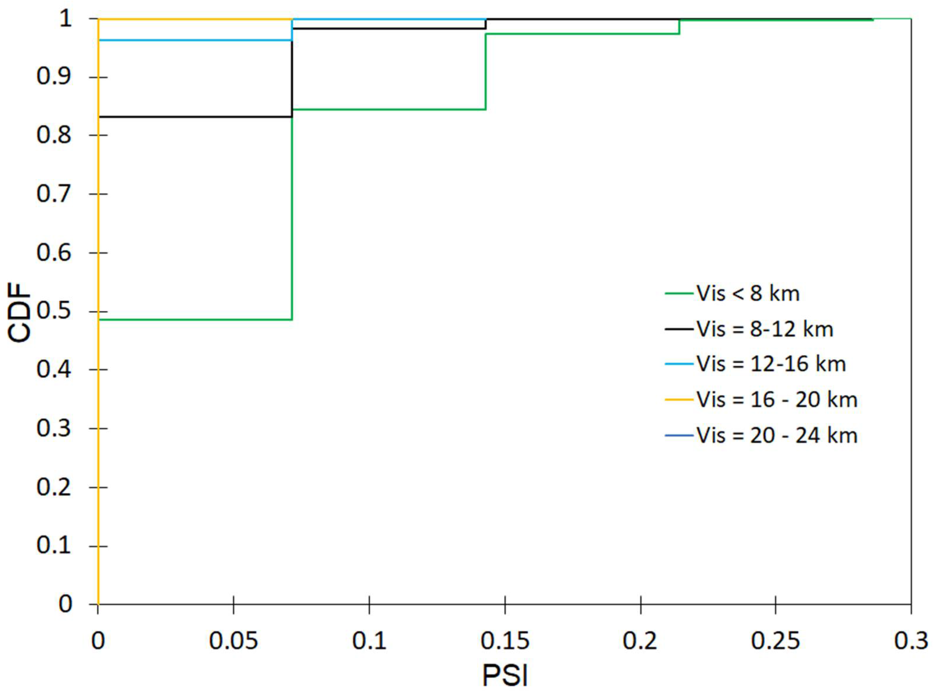
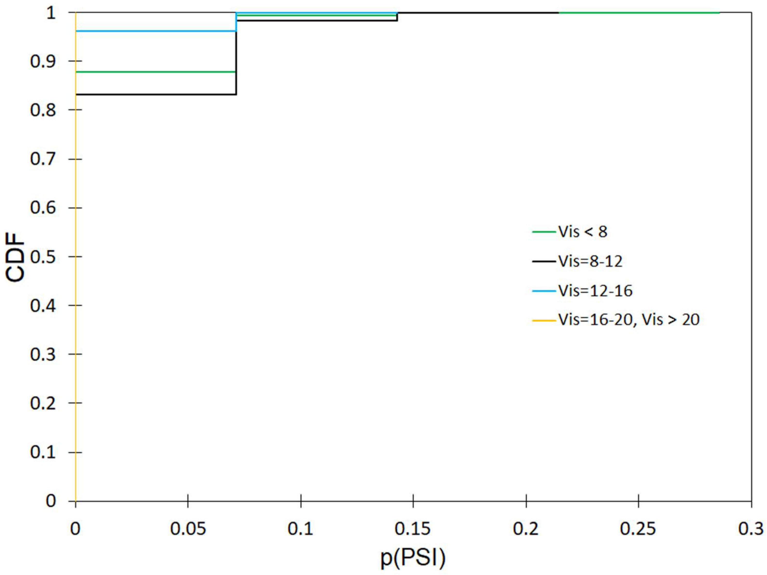
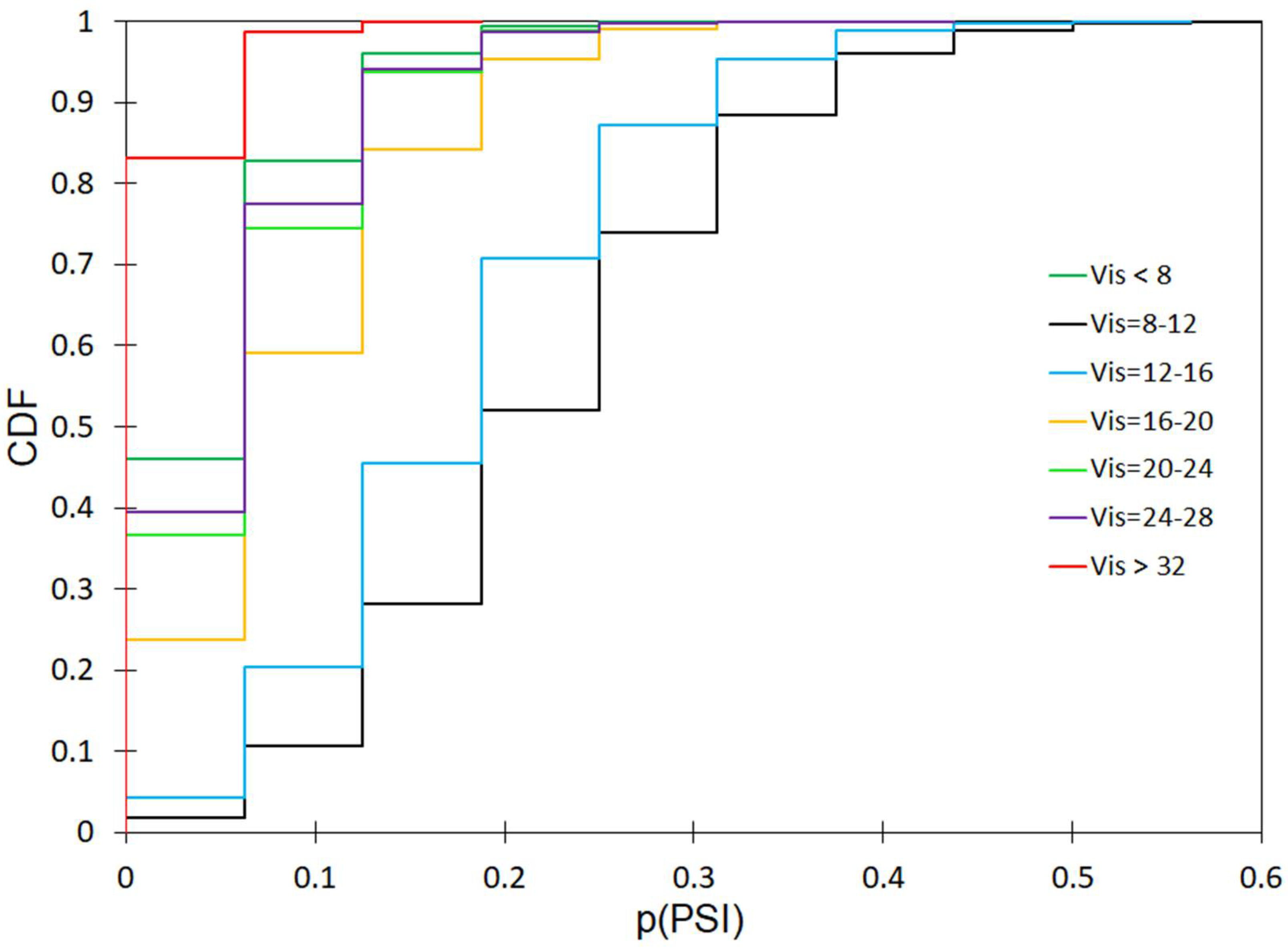
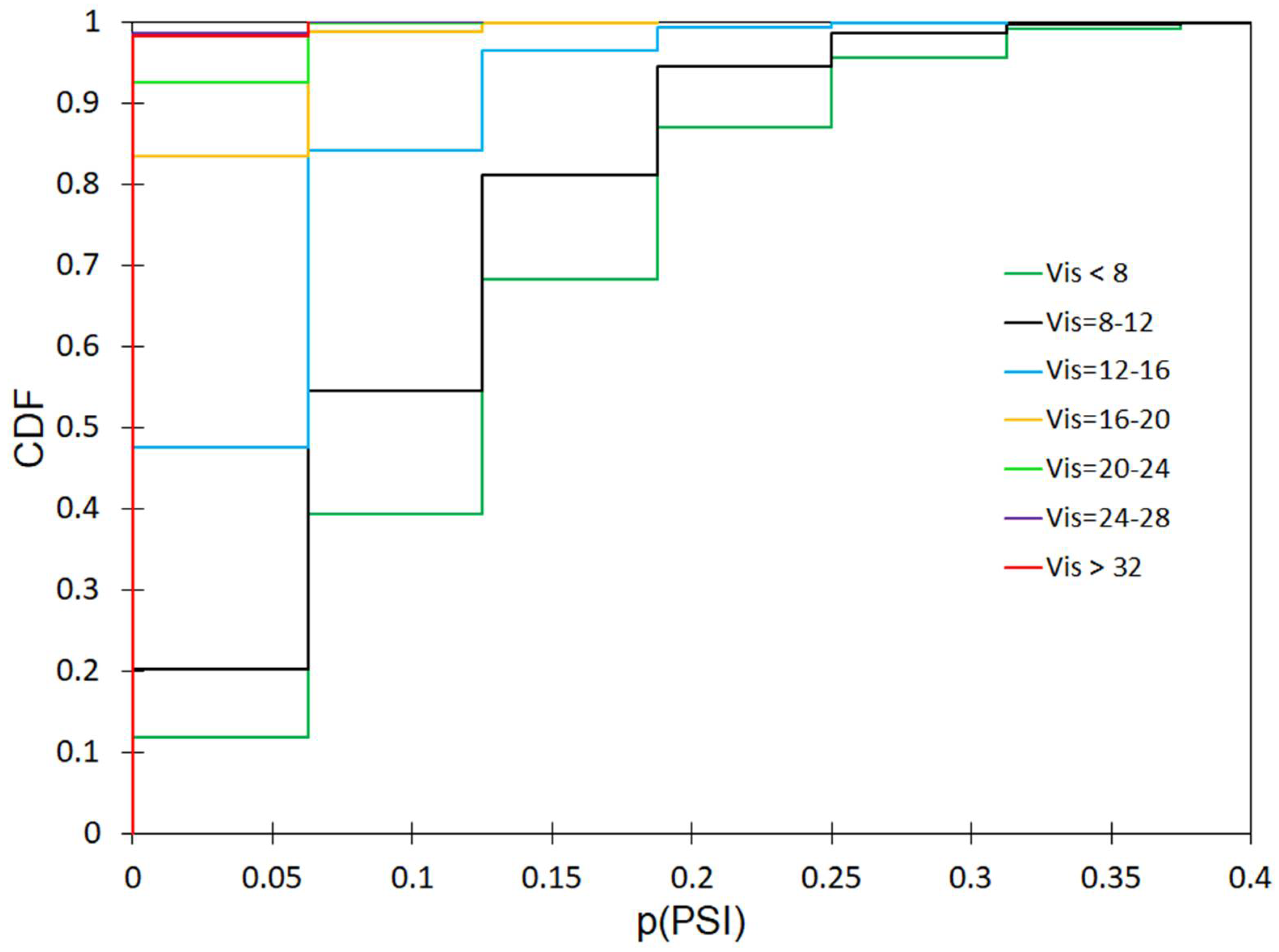
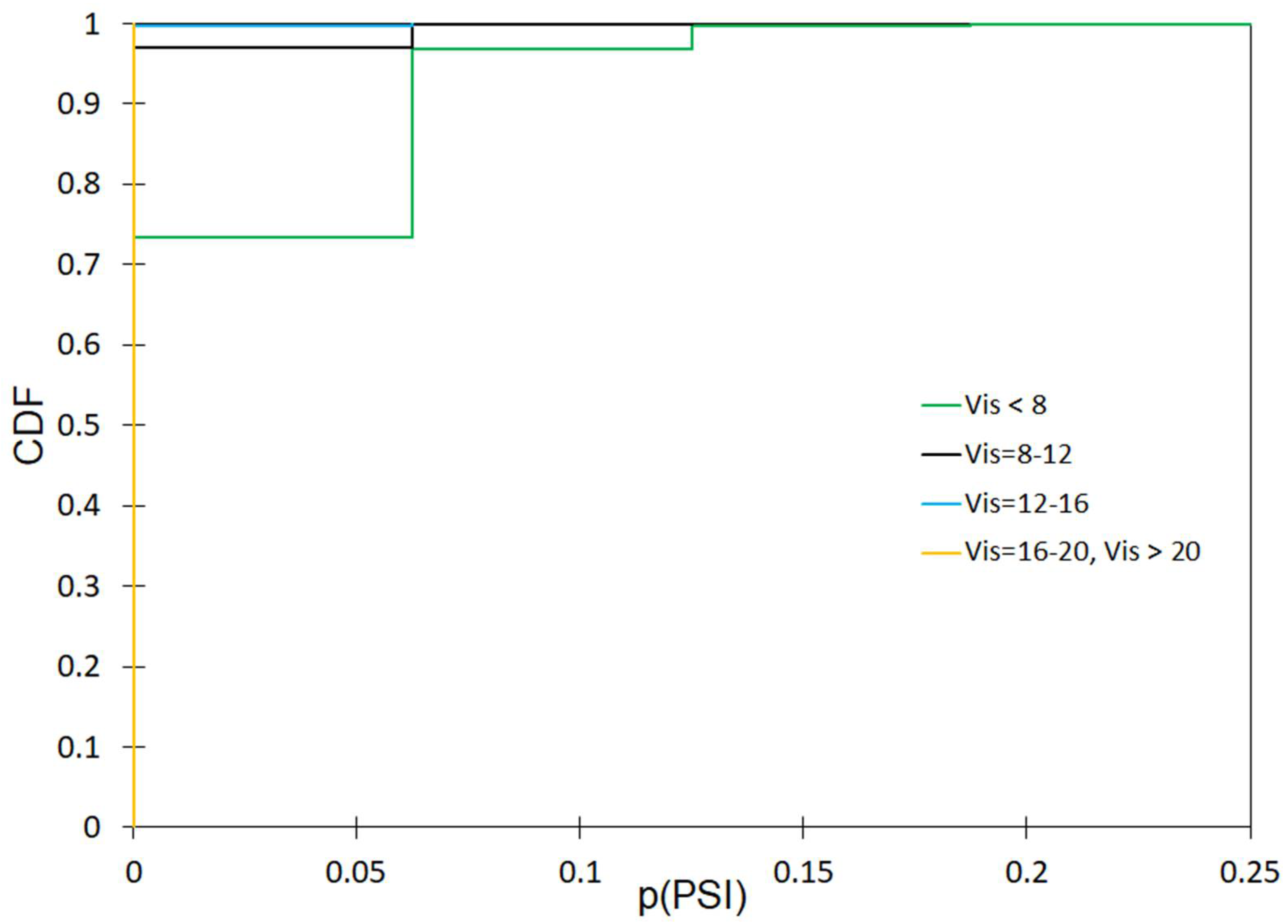
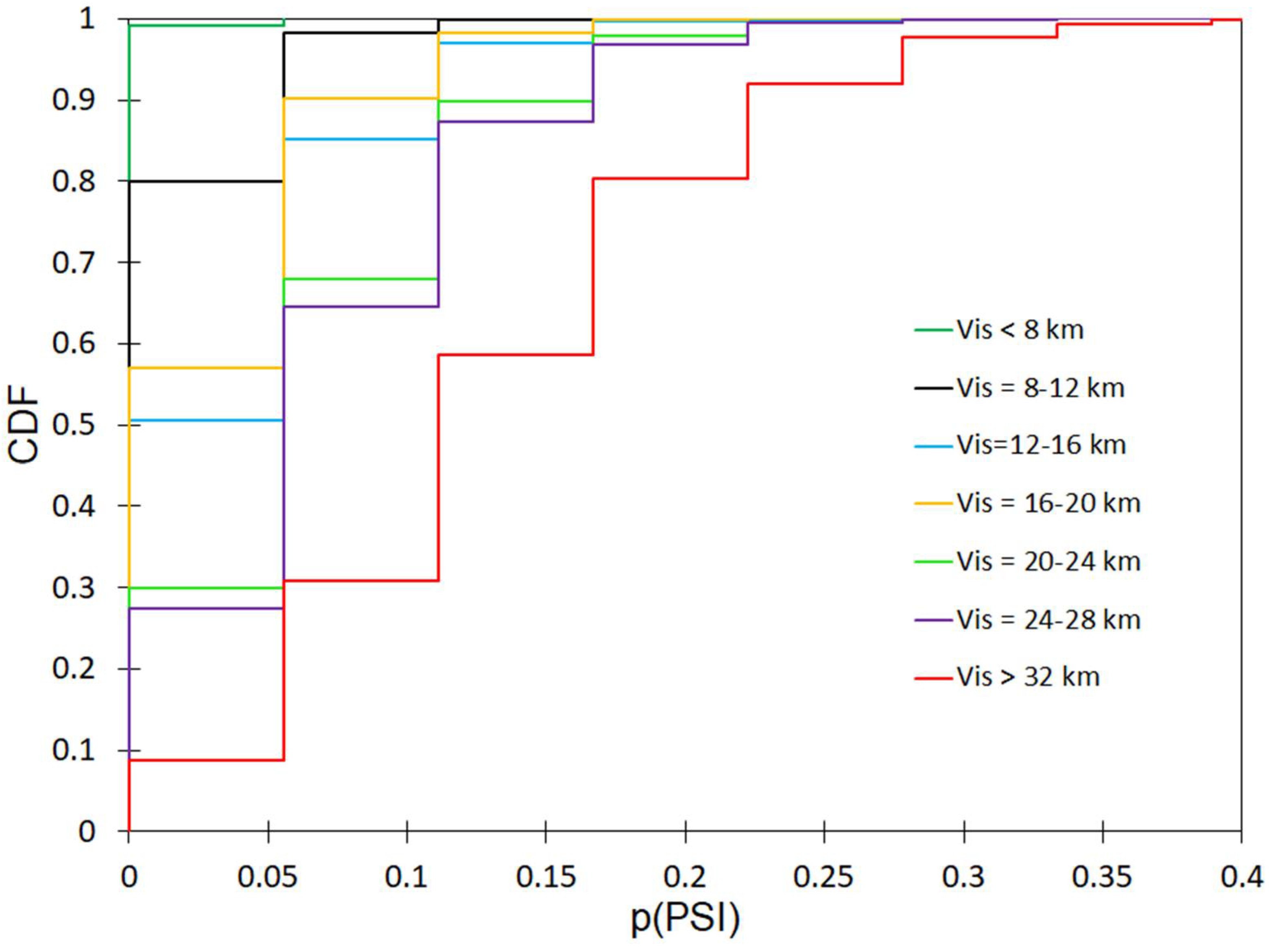
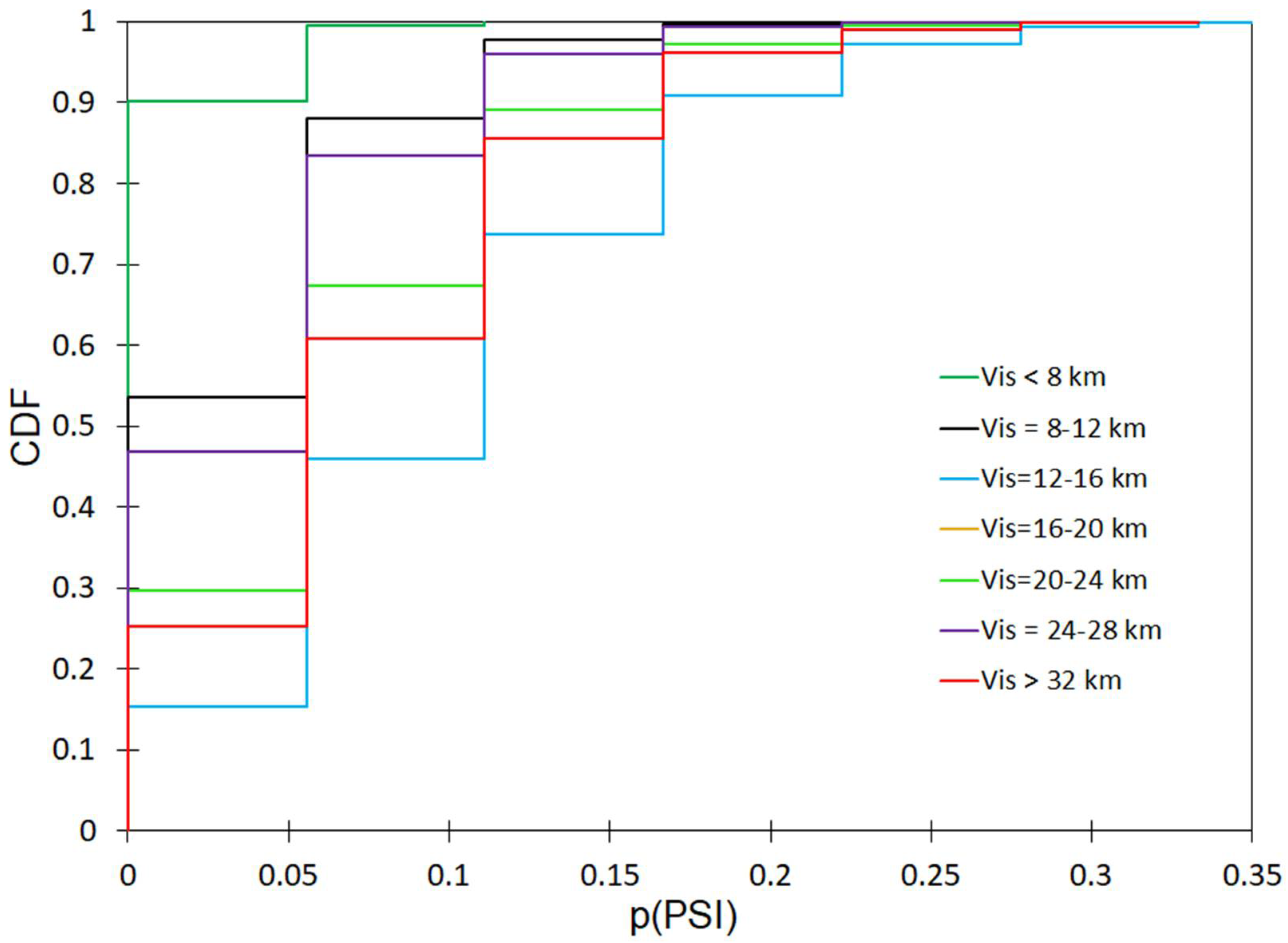
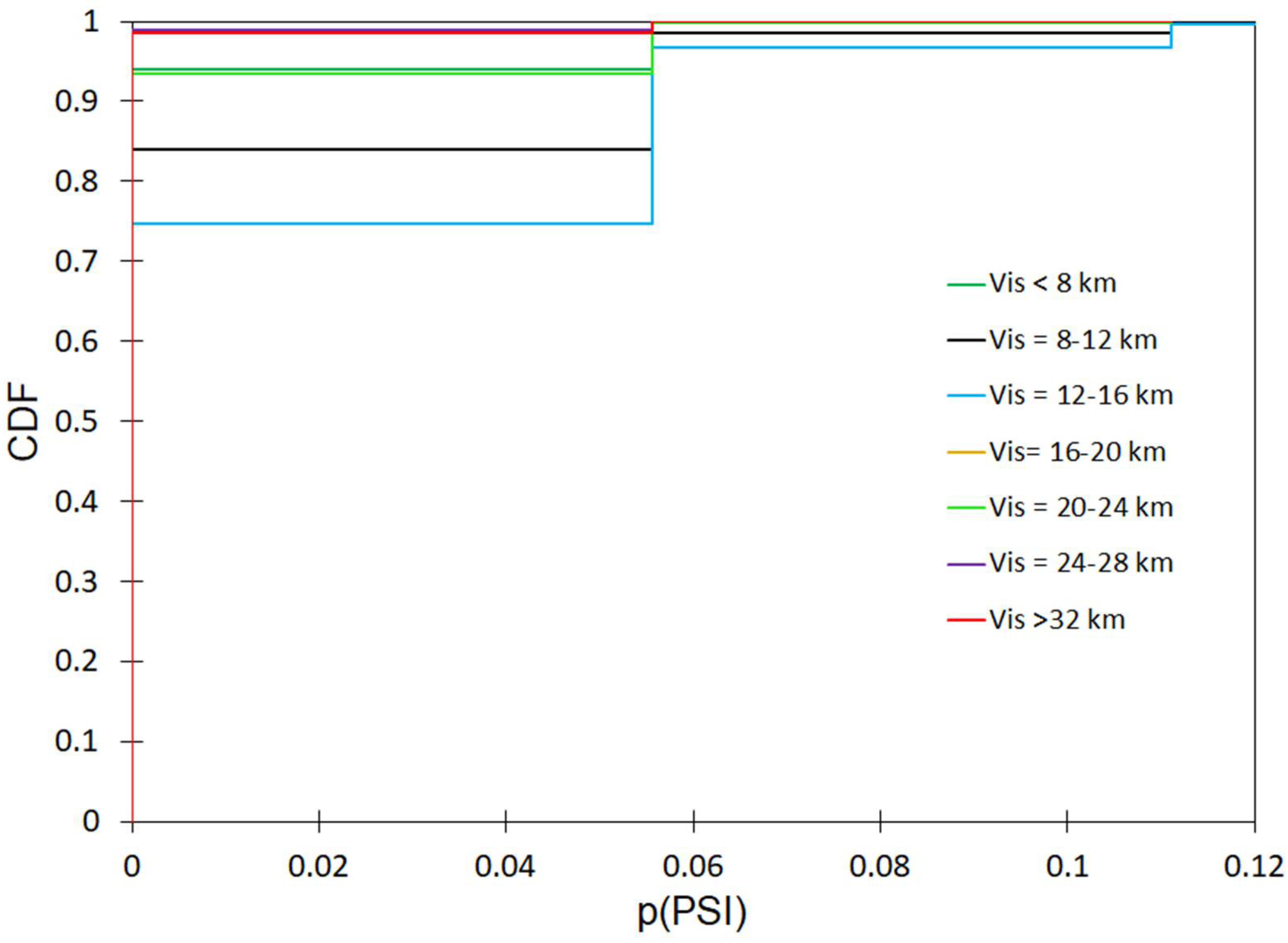
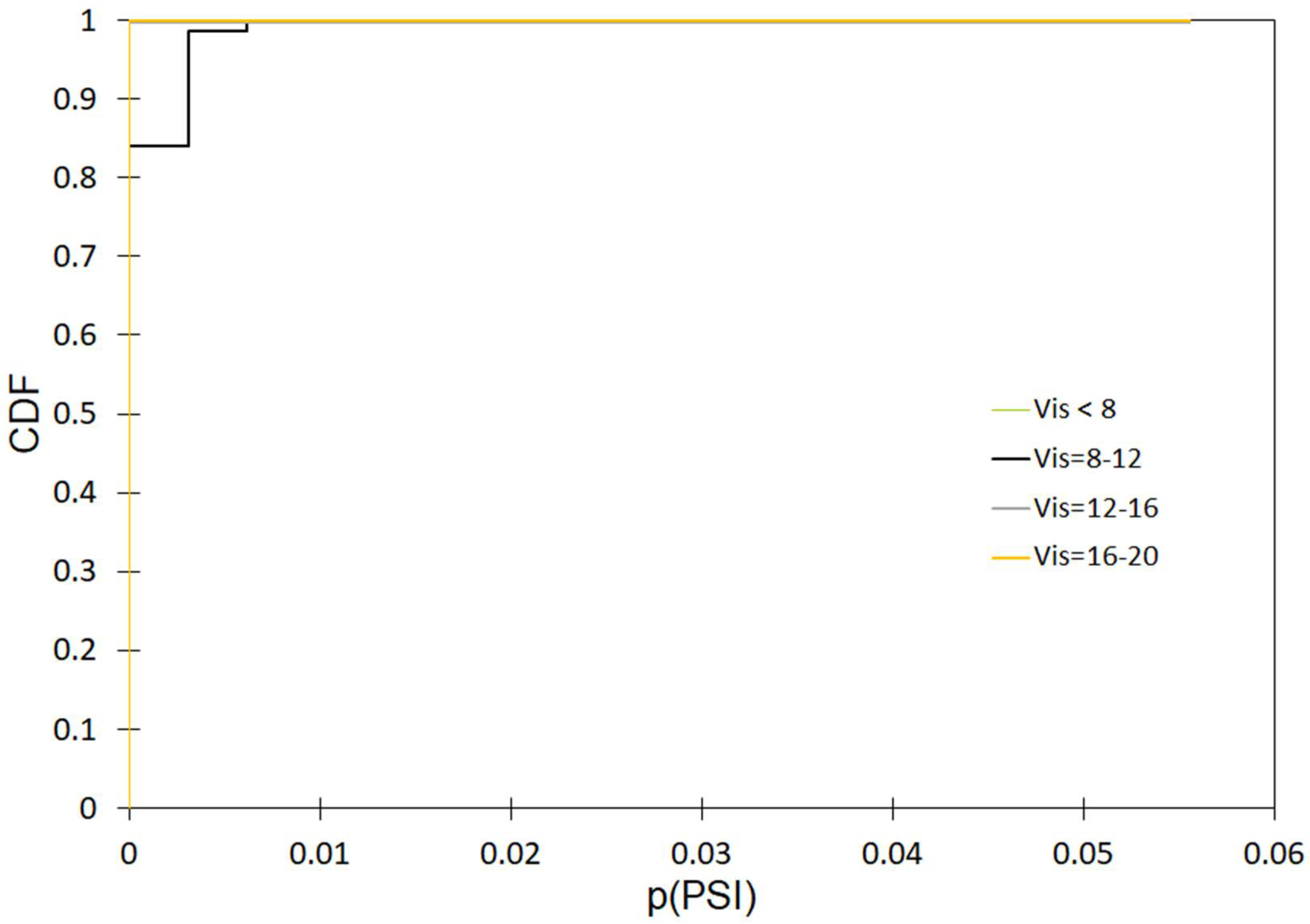
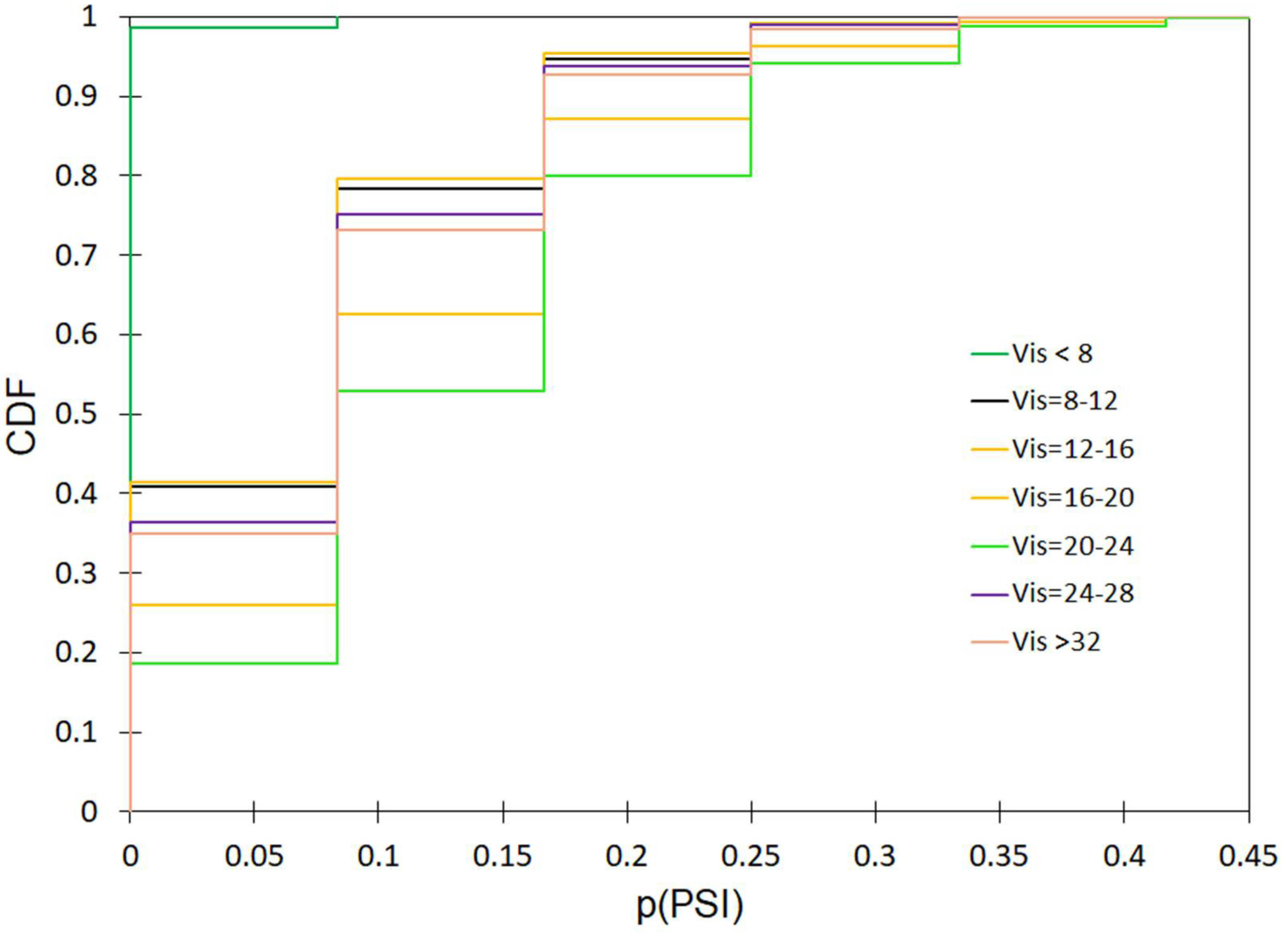
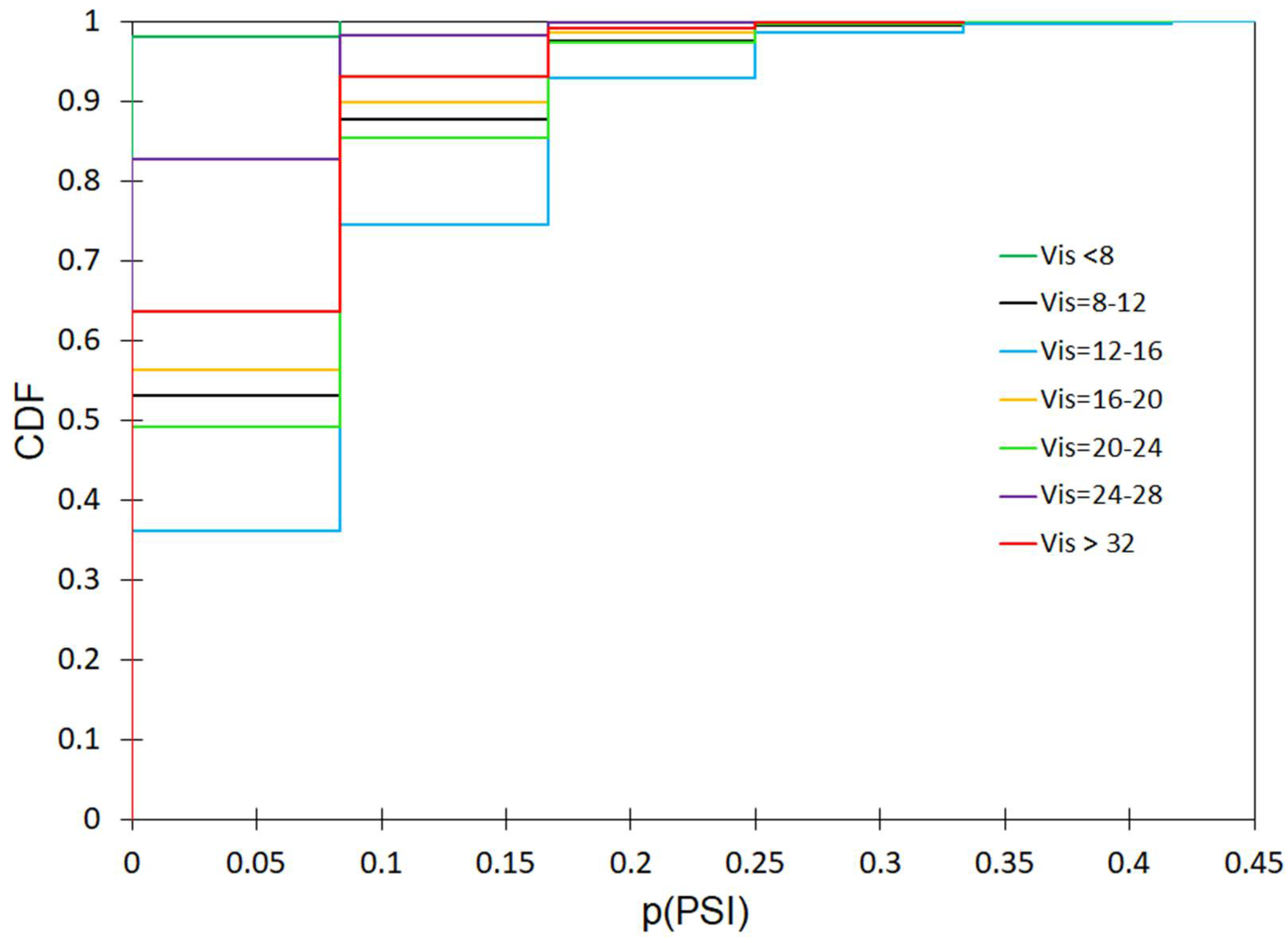
10.5. Influence of Visibility on the Air Pollution Index (API) over an Annual Cycle including Rainfall

On the basis of the prepared CDF curves (Figure 6), it was found that the cycle of annual changes in weather conditions, as well as air quality indices for wet and dry period has a great influence on API results. The calculation results for individual Vis values for the period of spring, summer and winter (wet and dry days) are provided in Figure A4, Figure A5 and Figure A6 in Appendix A.

The results of the Kolmogorov–Smirnov test probability calculations (

Table A4. Results of K-S calculations (probability p) showing the agreement of empirical and theoretical distributions describing the air quality index (API) in the corresponding range for precipitation and rain days for spring, summer and winter seasons.

Visibility	Spring Period		Summer Period		Winter Period
	Wet	Dry	Wet	Wet	Dry	Dry
Vis < 8	0.2216	0.2282	0.2033	0.2318	0.2336	0.2213
Vis = 8–12	0.2116	0.2350	0.2379	0.2134	0.2086	0.2015
Vis = 12–16	0.2262	0.2173	0.2051	0.2228	0.2147	0.2281
Vis = 16–20	0.2090	0.2129	0.2364	0.2258	0.2277	0.2394
Vis = 20–24	0.2348	0.2111	0.2145	0.2071	0.2180	0.2364
Vis = 24–28	0.2225	0.2040	0.2230	0.2354	0.2005	0.2216
Vis = 28–32	0.2003	0.2189	0.2228	0.2084	0.2223	0.2198
Vis > 32	0.2299	0.2059	0.2392	0.2214	0.2081	0.2371

) confirm the good fit between the determined theoretical distributions and the empirical ones. The calculated probability values are greater than acceptable values (p = 0.05); thus, there are no grounds to reject the assumption that the analyzed distributions are different. The conducted simulations showed that higher API values were obtained for the spring period than for the winter period, which is confirmed by the determined CDF curves. For example, the values of the 50% percentile for Vis < 8 km for the spring and summer period (dry season) are 6.37 and 5.57, respectively. In addition, for example, for the winter period (wet period) and Vis = 16–20 km, the value of API = 2.94, whereas for the spring period, it is equal to API = 3.74. The results of the analyses also confirmed the influence of the wet and dry period on the calculation results. For example, for the spring period and Vis = 16–20 km, the API value for wet weather is equal to 3.74 and for dry weather, it amounts to 4.66. The results obtained in this study are confirmed by the analysis conducted by Irani et al. [39], who, using the artificial neural network method, modeled the values of selected air quality indices (PM₁₀, NO₂, SO₂, CO, O₃) as input data for air quality index calculations also taking into account the amount of rainfall, wind speed and temperature.

10.6. Influence of Visibility on the Air Pollution Index (API) over an Annual Cycle including Rainfall

On the basis of logistic regression models and developed generators of air quality indices and weather conditions, the API values were calculated taking into account air visibility. Then, graphs showing the relationship between air quality indices (PM₁₀, SO₂, NO₂, O₃) and API, depending on the visibility values for wet and dry periods in the annual cycle were prepared. The results of the calculations (Figure 7) are presented for PM₁₀ (wet and dry period for winter) as the air quality index having the greatest impact on human health. The results of API calculations for other air quality indices (SO₂, NO₂, O₃) in the spring and summer periods for wet and dry weather are presented in Figure A7, Figure A8, Figure A9 and Figure A10 in Appendix A.

On the basis of the CDF curves in Figure 6, it can be concluded that for the dry period, larger API = f(Vis, PM₁₀) values were obtained than for the wet period. This is confirmed on the one hand by the PM₁₀ values, which do not exceed 11 μg·m⁻³ for the wet period and are lower than 14 μg·m⁻³ for the dry period. Simultaneously, for the wet period, the maximum API value is 125, while for the dry period, it is equal to 165 for Vis < 8 km. The obtained results confirm that the highest API variability was obtained for Vis < 8 km, regardless of whether the analyzed period was wet or dry, which may confirm the high variability of the values of modeled air quality indices in the dry and wet periods. The obtained calculation results confirm the large influence of visibility on the modeled API values. For example, for Vis < 8 km, the maximum API values for the wet period amounted to 125, while for Vis = 16–20 km and Vis > 32 km they were equal to 60 and 30, respectively. The identical relationship is shown for the wet period. In this case, the maximum API values for Vis = 16–20 km and Vis > 32 km were equal to 75 and 50, respectively. The simulations performed for the spring period (Figure A5) for the dry period showed a negligible effect of air visibility on the range of API variability. During this period, for Vis < 8 km to Vis < 32 km, maximum values of API = 112 were obtained. During the wet period (spring), the influence of air visibility on the API values was demonstrated. For Vis < 8 km, the maximum API values of 90 were obtained, while for Vis < 32 km, they reached no more than API = 60. The results of calculations for the summer period showed that for both wet and dry weather, maximum API values for Vis > 32 km were 62. The calculations performed for the summer period showed that for the given PM₁₀, values taking into account air visibility, smaller maximum API values were obtained for the wet period than for the dry period (Figure A5, Figure A6, Figure A7, Figure A8, Figure A9 and Figure A10 in Appendix A).

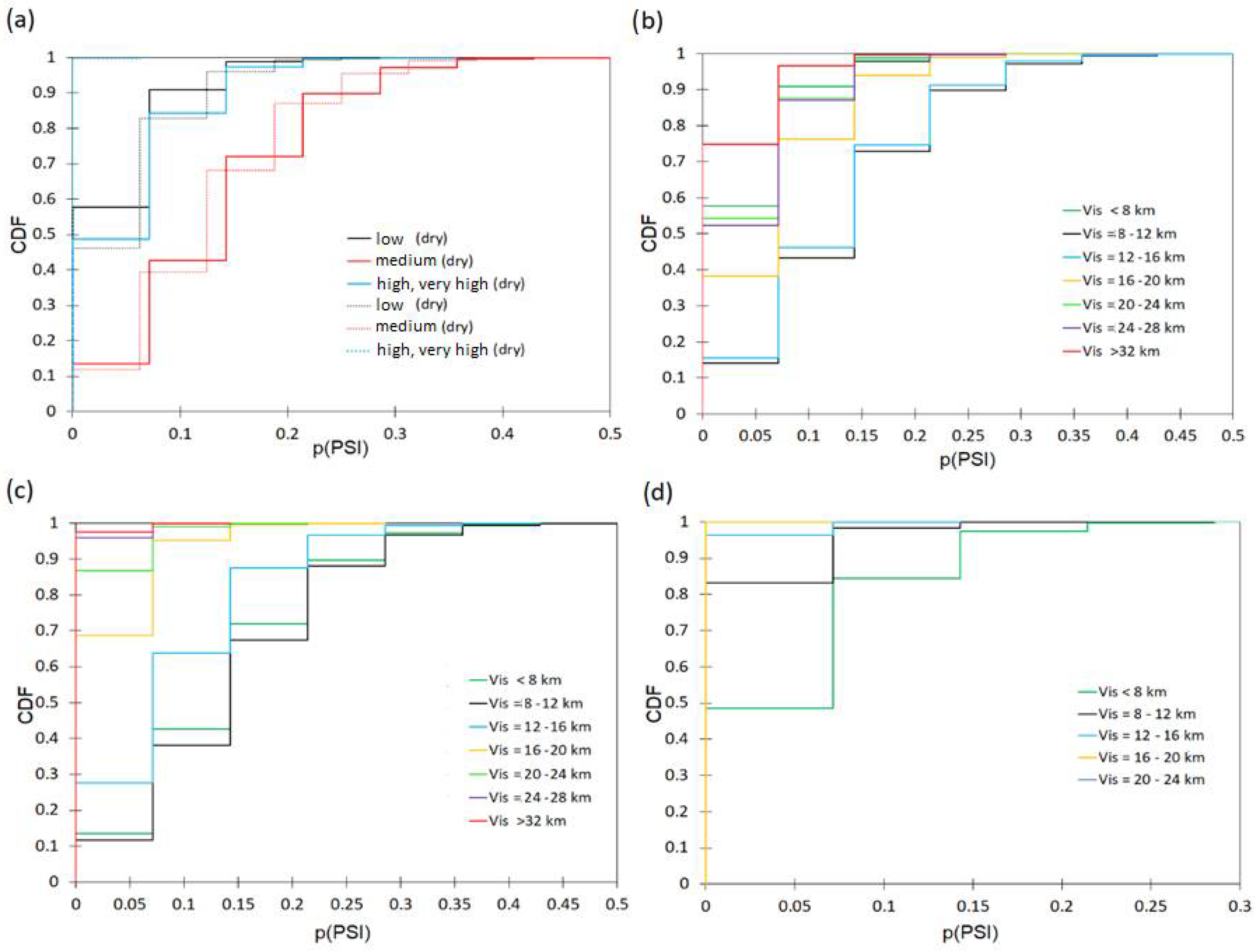
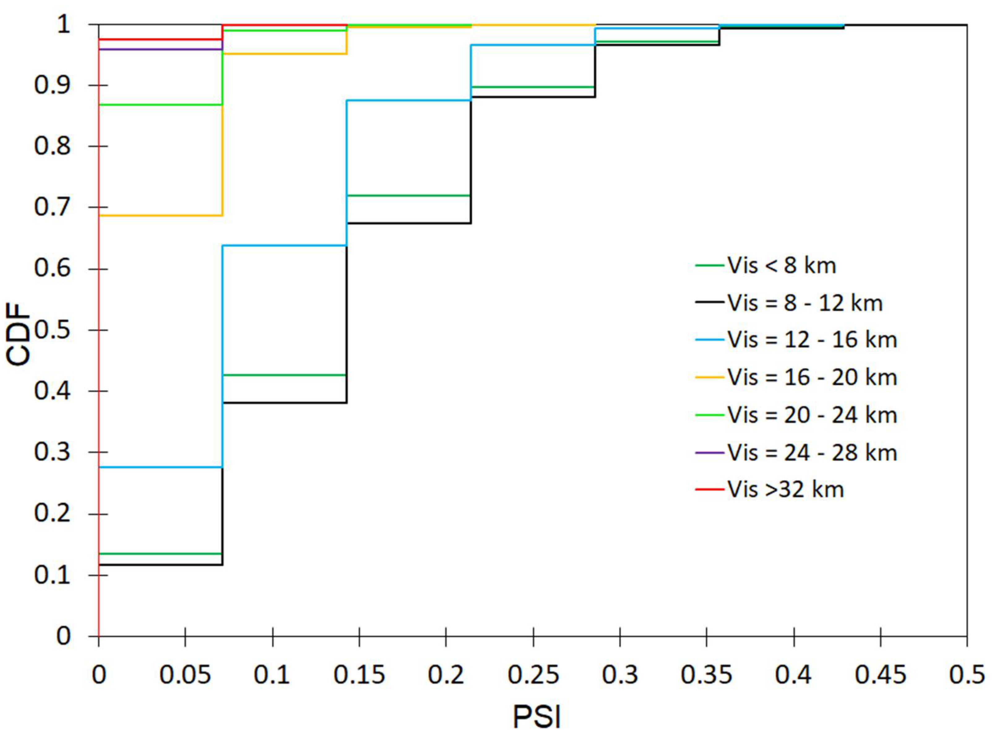
10.7. Effect of Visibility on Mortality Risk in an Annual Cycle

Using the determined logistic regression models, generators of selected air quality and weather conditions indices, calculations were performed for wet and dry periods in separated periods in the annual cycle. On this basis, the values of probability of exceeding the set Vis values, number of days with visibility in the appropriate variability range and API value were determined. Using these results, in accordance with the procedure described in the section “Calculation of AQI and API”, and the adopted division expressing the impact of API/PSI on human health, the frequency of occurrence of low, medium, high and very high mortality risk was determined in the calculation periods (Figure A11, Figure A12, Figure A13, Figure A14, Figure A15 and Figure A16 in Appendix A) The effect of rainfall conditions (wet, dry) on mortality risk for Vis < 8 km is provided in Figure 8a; the calculation results for the other options are provided in Figure A17, Figure A18, Figure A19, Figure A20, Figure A21, Figure A22, Figure A23, Figure A24, Figure A25, Figure A26, Figure A27, Figure A28, Figure A29, Figure A30, Figure A31, Figure A32, Figure A33, Figure A34, Figure A35, Figure A36, Figure A37, Figure A38 and Figure A39 in Appendix A. Figure 8b–d show the effect of visibility on the incidence of mortality risk for dry conditions; the calculation results for the wet period are provided in Appendix A.

It should be mentioned that the theoretical distributions obtained from the calculations were compared with the empirical distributions using the Kolmogorov–Smirnov test, yielding the test probability values above 0.05 (Table A3 in Appendix A), which indicates that there are no grounds to reject the hypothesis that the obtained distributions are consistent when compared with the measured data. On the basis of the CDF curves in Figure 8a, it was found that for wet conditions, lower values of mortality risk frequency were obtained for the separated groups (low, medium, high, very high). For example, the percentile value of 0.50 for the average mortality risk in the dry period is 0.14, while for the wet period, it is equal to 0.12. For the wet period, identical percentile values of the frequency of high and very high mortality risk were shown. On the basis of the obtained CDF curves, it was found that for Vis < 8 km for dry and wet weather (Figure 8a), the episodes with medium mortality risk were recorded most frequently, which is confirmed by the determined value of the percentile 0.50 equal to 0.14. In contrast, the episodes with low mortality risk are characterized by the lowest frequency of occurrence because the value of the percentile 0.50 is equal to 0, and for high/very high mortality risk, it amounts to 0.071. On the basis of the obtained CDF curves (Figure 8b–d), the tendency of low, medium and high mortality risk to decrease with increasing air visibility was shown. In addition, during the dry period, the complex influence of air visibility on the frequency of low mortality risk was shown; this is confirmed by the obtained values of p (PSI) percentiles. For the events with the low mortality risk, the highest incidence is characterized by the episodes when Vis = 8–12 km. This is confirmed by the 0.50 percentile value, which is 0.143.

Similar distributions were obtained for Vis = 12–16 km. In terms of the low incidence of mortality risk, it was shown that for Vis < 8 km as well as Vis = 20–28 km, similar distributions were obtained, which is confirmed in the CDF curves obtained. For the episodes of medium and high mortality risk, the highest incidence was shown in the dry period for Vis = 8–16 km and a clear decrease for Vis > 16 km. The lowest incidence was shown when Vis > 32 km, for which the percentile value of 0.50 is 0. For the dry period, the incidence of high mortality was confirmed, as indicated by the p (PSI) values, which is important in terms of the influence of air quality indices and weather conditions on human health. The obtained calculation results are confirmed by the analyses of Huang et al. [40], who showed for Shanghai that the risk of mortality due to cardiovascular and respiratory diseases decreases with increasing air visibility. This was also confirmed by the analysis of Shen et al. [41] for the Henan Province (China). Nevertheless, the approaches presented above do not provide a relationship in the form of a mathematical model between the determinants of health complaints and air quality, weather conditions and seasonality by year. The obtained results may be of great importance when assessing the impact of air quality on the human organism and trying to interpret them, taking into account, e.g., medical data, which may constitute the next stage of analyses in the developed computational tool. The proposed approach enables us to directly determine in a quantifiable way when the combination of weather factors and air quality may pose a threat to human health. This may be useful in the creation of early warning systems against the threats occurring as a result of adverse weather and climatic conditions.

11. Conclusions

Air visibility is one of the factors enabling us to assess, relate and interact between weather conditions (wet or dry) and air quality, which is important in terms of its impact on human health. The analyses performed in this study showed that air visibility can be modeled using a logistic regression model. Simultaneously, the influence of weather conditions and air quality indices varies depending on the value of air visibility. The adopted approach, compared to the currently used ones, enables us to study complex interactions between air quality and weather conditions in an annual cycle. The model developed in this paper allows determining the frequency of occurrence of visibility in a given range depending on air quality and weather conditions in an annual cycle, which is important in terms of assessing the quality of air. It was shown that in the wet period, the visibility of air increased in comparison to the dry period. Moreover, it was found that for the wet period in the monthly cycle, the number of days with visibility values of 8–32 km is lower than for the dry period. This relationship is determined by seasonality in the annual cycle. The analyses conducted showed a strong relationship between air visibility (depending on weather conditions) and air quality index. By determining the visibility, it is possible to identify the maximum API values, which is essential from the point of view of air quality assessment, but also its impact on human health. The results obtained in this study showed the relationships between air visibility and mortality, which is relevant for assessing the impact of weather conditions and air quality on the human organism and mortality. It was shown that an increase in visibility leads to a decrease in mortality, but this relationship is determined by seasonality in the annual cycle.

Considering the calculation results obtained with the developed mathematical model, further analyses are recommended to expand the algorithm and take into account local geographical conditions. It is important in terms of setting up a universal computational tool enabling us to analyze the influence of weather conditions and air quality in the context of mortality in a given area, e.g., the entirety of Poland, rather than a single location.

References

1. World Health Organization (WHO). Ambient Air Pollution: Health Impacts; World Health Organization: Geneva, Switzerland, 2016; Available online: https://www.who.int/publications/i/item/9789241511353 (accessed on 10 November 2021).
2. Kuo, C.-Y.; Cheng, F.-C.; Chang, S.-Y.; Lin, C.Y.; Chou, C.C.; Chou, C.-H.; Lin, Y.-R. Analysis of the major factors affecting the visibility degradation in two stations. J. Air Waste Manag. Assoc. 2013, 63, 433–441. [Google Scholar] [CrossRef] [PubMed] [Green Version]
3. Thach, T.-Q.; Wong, C.-M.; Chan, K.-P.; Chau, Y.-K.; Chung, Y.-N.; Ou, C.-Q.; Yang, L.; Hedley, A.J. Daily visibility and mortality: Assessment of health benefits from improved visibility in Hong Kong. Environ. Res. 2010, 110, 617–623. [Google Scholar] [CrossRef] [PubMed]
4. Liu, J.; Chen, E.; Zhang, Q.; Shi, P.; Gao, Y.; Chen, Y.; Liu, W.; Qin, Y.; Shen, Y.; Shi, C. The correlation between atmospheric visibility and influenza in Wuxi city, China. Medicine 2020, 99, e21469. [Google Scholar] [CrossRef] [PubMed]
5. Han, L.; Sun, Z.; He, J.; Hao, Y.; Tang, Q.; Zhang, X.; Zheng, C.; Miao, S. Seasonal variation in health impacts associated with visibility in Beijing, China. Sci. Total Environ. 2020, 730, 139149. [Google Scholar] [CrossRef] [PubMed]
6. Muhammad, S.; Long, X.; Salman, M. COVID-19 pandemic and environmental pollution: A blessing in disguise? Sci. Total Environ. 2020, 728, 138820. [Google Scholar] [CrossRef] [PubMed]
7. Yao, L.; Kong, S.; Zheng, H.; Chen, N.; Zhu, B.; Xu, K.; Cao, W.; Zhang, Y.; Zheng, M.; Cheng, Y.; et al. Co-benefits of reducing PM2.5 and improving visibility by COVID-19 lockdown in Wuhan. npj Clim. Atmos. Sci. 2021, 4, 40. [Google Scholar] [CrossRef]
8. Myllyvirta, L.; Thieriot, H. 11,000 Air Pollution-Related Deaths Avoided in Europe as Coal. Oil Consumption Plummet. 2020. Available online: https://energyandcleanair.org/wp/wp-content/uploads/2020/04/CREA-Europe-COVID-impacts.pdf (accessed on 10 November 2021).
9. Sahu, S.K.; Mangaraj, P.; Beig, G.; Tyagi, B.; Tikle, S.; Vinoj, V. Establishing a link between fine particulate matter (PM2.5) zones and COVID-19 over India based on anthropogenic emission sources and air quality data. Urban Clim. 2021, 38, 100883. [Google Scholar] [CrossRef]
10. Chung, Y.S.; Kim, H.S.; Yoon, M.B. Observations of Visibility and Chemical Compositions Related to Fog, Mist and Haze in South Korea. Water Air Soil Pollut. 1999, 111, 139–157. [Google Scholar] [CrossRef]
11. Kim, S.; Lee, S.; Hwang, K.; An, K. Exploring Sustainable Street Tree Planting Patterns to Be Resistant against Fine Particles (PM2.5). Sustainability 2017, 9, 1709. [Google Scholar] [CrossRef] [Green Version]
12. Zhao, Z.; Chen, S.-H.; Kleeman, M.J.; Tyree, M.; Cayan, D. The Impact of Climate Change on Air Quality–Related Meteorological Conditions in California. Part I: Present Time Simulation Analysis. J. Clim. 2011, 24, 3344–3361. [Google Scholar] [CrossRef] [Green Version]
13. Zhang, F.; Chen, J.; Qiu, T.; Yin, L.; Chen, X.; Yu, J. Pollution Characteristics of PM2.5 during a Typical Haze Episode in Xiamen, China. Atmos. Clim. Sci. 2013, 3, 427–439. [Google Scholar] [CrossRef] [Green Version]
14. Deng, J.; Wang, T.; Jiang, Z.; Xie, M.; Zhang, R.; Huang, X.; Zhu, J. Characterization of visibility and its affecting factors over Nanjing, China. Atmos. Res. 2011, 101, 681–691. [Google Scholar] [CrossRef]
15. Du, K.; Mu, C.; Deng, J.; Yuan, F. Study on atmospheric visibility variations and the impacts of meteorological parameters using high temporal resolution data: An application of Environmental Internet of Things in China. Int. J. Sustain. Dev. World Ecol. 2013, 20, 238–247. [Google Scholar] [CrossRef]
16. Tsai, Y.I.; Kuo, S.-C.; Lee, W.-J.; Chen, C.-L.; Chen, P.-T. Long-term visibility trends in one highly urbanized, one highly industrialized, and two Rural areas of Taiwan. Sci. Total Environ. 2007, 382, 324–341. [Google Scholar] [CrossRef]
17. Majewski, G.; Rogula-Kozłowska, W.; Czechowski, P.O.; Badyda, A.; Brandyk, A. The Impact of Selected Parameters on Visibility: First Results from a Long-Term Campaign in Warsaw, Poland. Atmosphere 2015, 6, 1154–1174. [Google Scholar] [CrossRef] [Green Version]
18. Savapandit, M.R.R.; Gogoi, D.B. Bootstrap and Other Tests For Goodness of Fit. Sci. Math. Jpn. 2015, 78, 99–110. [Google Scholar] [CrossRef]
19. Pyta, H. Classification of air quality based on factors of relative risk of mortality increase. Environ. Prot. Eng. 2008, 34, 111–117. [Google Scholar]
20. Cairncross, E.K.; John, J.; Zunckel, M. A novel air pollution index based on the relative risk of daily mortality associated with short-term exposure to common air pollutants. Atmos. Environ. 2007, 41, 8442–8454. [Google Scholar] [CrossRef]
21. World Health Organization (WHO). The World Health Report 2001—Mental Health: New Understanding, New Hope; World Health Organization: Geneva, Switzerland, 2001; Volume 79, p. 1085. [Google Scholar]
22. Majewski, G.; Szeląg, B.; Mach, T.; Rogula-Kozłowska, W.; Anioł, E.; Bihałowicz, J.; Dmochowska, A.; Bihałowicz, J.S. Predicting the Number of Days with Visibility in a Specific Range in Warsaw (Poland) Based on Meteorological and Air Quality Data. Front. Environ. Sci. 2021, 9, 623094. [Google Scholar] [CrossRef]
23. Rodriguez, M.Z.; Comin, C.H.; Casanova, D.; Bruno, O.M.; Amancio, D.R.; Costa, L.D.F.; Rodrigues, F. Clustering algorithms: A comparative approach. PLoS ONE 2019, 14, e0210236. [Google Scholar] [CrossRef]
24. Kassambara, A. Multivariate Analysis I: Practical Guide to Cluster Analysis in R. Unsupervised Machine Learning; CreateSpace Independent Publishing Platform: Scotts Valley, CA, USA, 2017; p. 188. [Google Scholar]
25. Jorquera, H.; Villalobos, A.M. Combining Cluster Analysis of Air Pollution and Meteorological Data with Receptor Model Results for Ambient PM2.5 and PM10. Int. J. Environ. Res. Public Health 2020, 17, 8455. [Google Scholar] [CrossRef] [PubMed]
26. Saksena, S.; Joshi, V.; Patil, R.S. Cluster analysis of Delhi’s ambient air quality data. J. Environ. Monit. 2003, 5, 491–499. [Google Scholar] [CrossRef] [PubMed]
27. Oleniacz, R.; Gorzelnik, T. Assessment of the Variability of Air Pollutant Concentrations at Industrial, Traffic and Urban Background Stations in Krakow (Poland) Using Statistical Methods. Sustainability 2021, 13, 5623. [Google Scholar] [CrossRef]
28. Harrell, F.E. Regression Modeling Strategies: With Applications to Linear Models, Logistic Regression, and Survival Analysis; Springer: Berlin/Heidelberg, Germany, 2001; Available online: https://link.springer.com/book/10.1007/978-1-4757-3462-1 (accessed on 10 November 2021).
29. Bagley, S.C.; White, H.; Golomb, B.A. Logistic regression in the medical literature:: Standards for use and reporting, with particular attention to one medical domain. J. Clin. Epidemiol. 2001, 54, 979–985. [Google Scholar] [CrossRef]
30. Stojić, S.S.; Stanišić, S.; Stojić, A. Temperature-related mortality estimates after accounting for the cumulative effects of air pollution in an urban area. Environ. Health 2016, 15, 73. [Google Scholar] [CrossRef] [PubMed] [Green Version]
31. Oguntunde, P.E.; Odetunmibi, O.A.; Adejumo, A.O. A Study of Probability Models in Monitoring Environmental Pollution in Nigeria. J. Probab. Stat. 2014, 2014, 864965. [Google Scholar] [CrossRef] [Green Version]
32. Iman, R.L.; Conover, W.J. A distribution-free approach to inducing rank correlation among input variables. Commun. Stat.-Simul. Comput. 1982, 11, 311–334. [Google Scholar] [CrossRef]
33. Singh, A.; George, J.P.; Iyengar, G.R. Prediction of fog/visibility over India using NWP Model. J. Earth Syst. Sci. 2018, 127, 26. [Google Scholar] [CrossRef] [Green Version]
34. Lee, H.-H.; Iraqui, O.; Gu, Y.; Yim, S.H.-L.; Chulakadabba, A.; Tonks, A.Y.-M.; Yang, Z.; Wang, C. Impacts of air pollutants from fire and non-fire emissions on the regional air quality in Southeast Asia. Atmos. Chem. Phys. 2018, 18, 6141–6156. [Google Scholar] [CrossRef] [Green Version]
35. Baklanov, A.; Zhang, Y. Advances in air quality modeling and forecasting. Glob. Transit. 2020, 2, 261–270. [Google Scholar] [CrossRef]
36. So, R.; Teakles, A.; Baik, J.; Vingarzan, R.; Jones, K. Development of visibility forecasting modeling framework for the Lower Fraser Valley of British Columbia using Canada’s Regional Air Quality Deterministic Prediction System. J. Air Waste Manag. Assoc. 2018, 68, 446–462. [Google Scholar] [CrossRef] [PubMed]
37. Pan, H.; Xue, J.; Huang, M.; Lei, X. Air Visibility Prediction Based on Multiple Models. In Proceedings of the 2018 IEEE 8th Annual International Conference on CYBER Technology in Automation, Control, and Intelligent Systems (CYBER), Tianjin, China, 19–23 July 2018; pp. 1421–1426. [Google Scholar] [CrossRef]
38. Berger, V.W.; Zhou, Y. Kolmogorov–Smirnov Test: Overview; Wiley StatsRef: Statistics Reference Online; John Wiley & Sons: Hoboken, NJ, USA, 2014. [Google Scholar] [CrossRef]
39. Irani, T.; Hamid, A.; Hedieh, D. Evaluating Visibility Range on Air Pollution using NARX Neural Network. J. Environ. Treat. Tech. 2020, 9, 540–547. [Google Scholar] [CrossRef]
40. Huang, W.; Tan, J.; Kan, H.; Zhao, N.; Song, W.; Song, G.; Chen, G.; Jiang, L.; Jiang, C.; Chen, R.; et al. Visibility, air quality and daily mortality in Shanghai, China. Sci. Total Environ. 2009, 407, 3295–3300. [Google Scholar] [CrossRef] [PubMed]
41. Shen, F.; Ge, X.; Hu, J.; Nie, D.; Tian, L.; Chen, M. Air pollution characteristics and health risks in Henan Province, China. Environ. Res. 2017, 156, 625–634. [Google Scholar] [CrossRef] [PubMed]
42. R Core Team. R: A Language and Environment for Statistical Computing; R Foundation for Statistical Computing: Vienna, Austria, 2020; Available online: https://www.R-project.org/ (accessed on 5 July 2021).
43. Murdoch, D.; Adler, D. rgl: 3D Visualization Using OpenGL. R Package Version 0.107.14. 2020. Available online: https://CRAN.R-project.org/package=rgl (accessed on 5 July 2021).
Figure 1. Location of the air quality, meteorological and visibility stations in the enlarged map of Warsaw with a map of Poland (Foto 1: Vis = 14 km; Foto 2: Vis = 3.7 km).
Energies 14 08397 g001
Figure 2. Model algorithm for analyzing the effect of visibility on the API for precipitation and dry days on an annual basis.
Energies 14 08397 g002
Figure 3. Results of cluster analysis for the analyzed measurement point.
Energies 14 08397 g003
Figure 4. Variability of visibility (Vis) over the annual cycle.
Energies 14 08397 g004
Figure 5. Number of days (N) over a two-week period in the variability range Vis = 8–32 km for dry and wet weather for the period: (a) spring; (b) summer; (c) winter.
Energies 14 08397 g005
Figure 6. Effect of visibility (Vis), period in annual cycle depending on wet and dry weather on API.
Energies 14 08397 g006
Figure 7. Influence PM10 air concentration depending on the air quality index for (a) wet and (b) dry periods in winter season.
Energies 14 08397 g007
Figure 8. Effect of rainfall conditions on the incidence of winter mortality risk for Vis < 8 km. Effect of visibility on the incidence of mortality risk: (a) low; (b) medium; (c) high; (d) very high for the dry period.
Energies 14 08397 g008