Agricultural Production on Erosion-Affected Land from the Perspective of Remote Sensing

Abstract

In this article, we discuss the influence of soil erosion on crop yield in the erosion-prone chernozem region of South Moravia. Erosional and depositional areas show significant differences in soil properties, which are also reflected in total crop yield. Plots of winter wheat, grown during the years 2016–2019 were used for analysis. The Enhanced Vegetation Index (EVI), referred to in literature as one of the best correlates of yield, was used to provide indirect information on yield. Although erosional areas are visible on orthophoto images on chernozem soils, the necessary orthophoto images are not always available. Thus, we have proposed a method for the identification of such erosion-affected areas based on the use of Sentinel 2 satellite images and NDVI or NBR2 indices. The relationship between yield and erosion was expressed through Pearson’s correlation on a sample of pixels randomly selected on the studied plots. The results showed a statistically significant linear reduction in yield depending on the level of degradation. All plots were further reclassified, according to level of degradation, as high, medium, or low state of degradation, where the average EVI values were subsequently calculated. Yield on non-degraded soil is 16 ± 1% higher on average.

1. Introduction

Soil erosion has a detrimental effect on global soil resources, soil sustainability, and food security [1]. During the last 40 years, nearly one-third of the world’s arable land has been lost through erosion and the on-site cost of water erosion in the United States of America is estimated to be about US $16 billion per year, based on expert knowledge [2]. In Europe, about one-third of land also suffers a high to very high risk of water erosion [3], and the productivity loss due to soil erosion in the European Union is estimated to be around € 300 million [4]. A recent estimation of land degradation costs shows that the global economic impact is highly uncertain, from US $40 to 490 billion, and varies from country to country [5]. Sartori et al. [6] state that soil erosion by water is estimated to incur a global annual cost of US $8 billion to global GDP.

Several studies describe the impact of agricultural activity on erosion processes (e.g., [7,8,9,10]) and this soil erosion generates on-site costs, which directly affect farming, for example through loss of fertile land and decline in soil resources [11]. There is a reduction in yield, loss of nutrients, reduction in the available planting area, etc. [12]. Erosion not only alters soil properties and removes nutrients, but also significantly affects crop yield [13,14]. Differences in the effect of erosion on productivity loss can be significant and related to many natural and anthropogenic factors. Panagos et al. [4] show the estimated annual productivity loss for individual EU countries, with the greatest losses in Europe occurring in the southern countries, and less influence in central and northern Europe. Additionally, Bakker et al. [15] describe how productivity in northern Europe is not as significantly reduced by water erosion as in southern countries. Similar conclusions are published by van den Born et al. and de la Rossa et al. [3,16], with the proviso that in these areas the risk may increase in the future. At the same time, soil erosion is a long-term problem, but it requires a solution in the short term [17].

There are currently a large number of publications on erosion problems, and many publications on erosion processes and crop yield (e.g., [18,19]). This reduction in yield on erosion-prone land is due to a reduction in the depth of the overlying horizons, nutrient loss, and changes in the physical properties of the soil [20,21,22]. There is, however, a limited amount of quantitative information on the effect of past and future erosion on agricultural productivity at a regional and national level [23,24].

There are various ways to study this problem. It is possible to evaluate, e.g., the price of soil [25], a decline in crop production due to soil erosion, or use macroeconomic models. Methods of assessing the decline in crop production include artificially removing topsoil, referred to as desurfacing, or, conversely, adding topsoil to eroded soils. Some studies compare yield along a transect, or compare plots with varying degrees of erosion [3,15,18,26,27]. Crop yield is affected by loss of nutrients due to erosion processes, and their replacement is calculated by, e.g., Martínez-Casasnovas and Ramos [14]. It is also possible to quantify the cost of erosion control measures (e.g., [28,29]). Research data obtained, together with other statistical data, can be used for macroeconomic models estimating the cost of soil erosion in agriculture [4].

With the development of technical possibilities, the tools of remote sensing (RS) are increasingly used, in relation to the estimation of crop yield, when searching for yield correlates, or even suitable indices for distinguishing individual crops. One of the most commonly mentioned indices concerning crop yield is the normalized difference vegetation index (NDVI) and the enhanced vegetation index (EVI) [30,31,32,33]. The NDVI is based on the red and near-infrared parts of the spectrum, and the EVI adds the blue part of the electromagnetic spectrum.

In the research articles, various approaches concerning the season period of remote sensing are mentioned to estimate yield (average, maximum values for the period, specific values at the beginning or end, or in the middle of the season) [34].

Remote sensing can also be successfully used to obtain information on spatial structural patterns of bare soil [35], as well as to define the rate of erosion, especially on chernozem soils [36]. From this point of view, aerial remote sensing, with high resolution, is the ideal option.

Despite the significant expansion of remote sensing, to the authors’ knowledge, there is a lack of publications relating to remote-sensing of indices of crop yield in connection with erosion factors. This is the main goal of the presented research. In addition, there are currently few studies focusing on understanding the economic context of erosion that would provide information for farmers and/or policymakers to consider the problem and implement conservation measures [14,26]. Analysis of local impacts and the cost of land degradation is important for understanding farmers’ responses to land degradation [37] and the resources they are losing. Therefore, in our research, we have focused on the issue of erosion processes on chernozem soils in the production area of South Moravia with the use of remote sensing tools, enabling analysis of a larger area in a broader time horizon.

2. Material and Methods

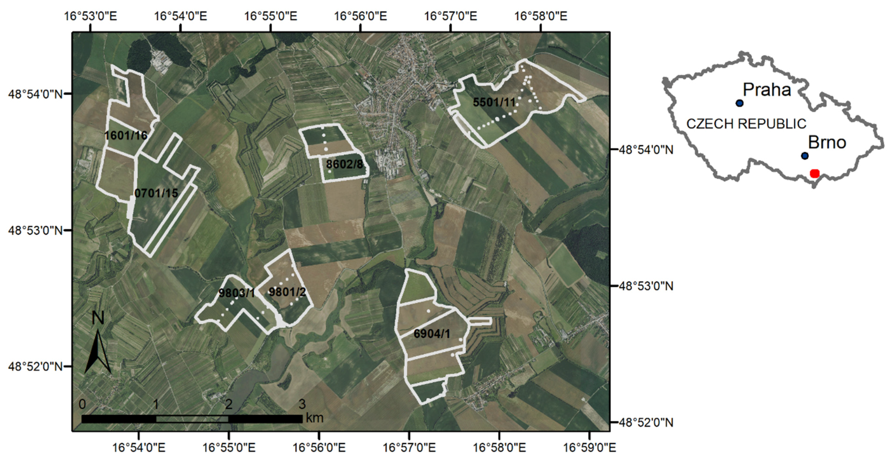
2.1. Study Area and Soil Properties

The research interest area is located in the agricultural region of South Moravia, with the dominant soil type of Chernozems [38]. The site is located at coordinates 48.89 N, 16.94 E, and in the vicinity of 10 km (Figure 1).

Within this area, plots were selected on which winter wheat was grown in the years 2016–2019 (1102 hectares in total). Wheat was chosen because it is the most cultivated crop in the region, making up about 37% of crop rotation. The evaluated area of winter wheat was cultivated in conventional manner and the individual plots were fertilized with the same dose of nutrients over the whole plot. In the case of nitrogen, the dosage was 140–160 kg N/ha depending on the year. Likewise, the same agricultural technology and plant protection were always applied across the whole plot.

Samples from the soil horizon of 0–20 cm were collected in the erosional and depositional zones in this area, and were analyzed to determine differences in soil properties in the erosion-affected areas. The selected soil characteristics were determined according to the following procedures: physical characteristics, such as bulk density, total porosity, maximum capillary water capacity, and minimum air capacity, were determined after sampling into Kopecky cylinders. Physical properties were determined using the standard method of Zbíral and Honsa [39]. The stability of soil aggregates was determined by wet sieving [40]. Chemical characteristics, such as the content of available phosphorus and calcium, were determined using the extraction solution according to Mehlich III, followed by atomic absorption spectrophotometry, atomic emission spectrophotometry, and photometry [39,41]. Total organic carbon (C_org.) content was determined by soil oxidation with a chromosulfuric mixture and color intensity was then measured by spectrophotometry [42,43]. Total nitrogen (N_tot.) was determined by oxidation of nitrogen peroxide in a concentrated sulfuric acid environment. After mineralization, distillation into boric acid was carried out and the crude protein content was determined by titration with H₂SO₄ [43,44]. Soil reaction was determined as pH/H₂O [39,45]. The humus fractions were determined by a modified procedure of Kononova and Běličkova [46]. Soil enzyme activity was determined by means of colorimetric ending. Cellulase activity was determined using CM-cellulose as a substrate [47], phosphatase activity using p-nitrophenyl phosphate as a substrate [48], triphenyl tetrazolium chloride was a substrate for the determination of dehydrogenase activity [49], and, in order to determine urease activity, incubation was carried out with a urea solution [50].

2.2. Data Processing

The methodological approach assumes that wheat yield on chernozem soil correlates with the EVI index obtained from remote sensing. This has been verified in specific locations where yield maps are available. The procedure consisted of several steps:

(1)

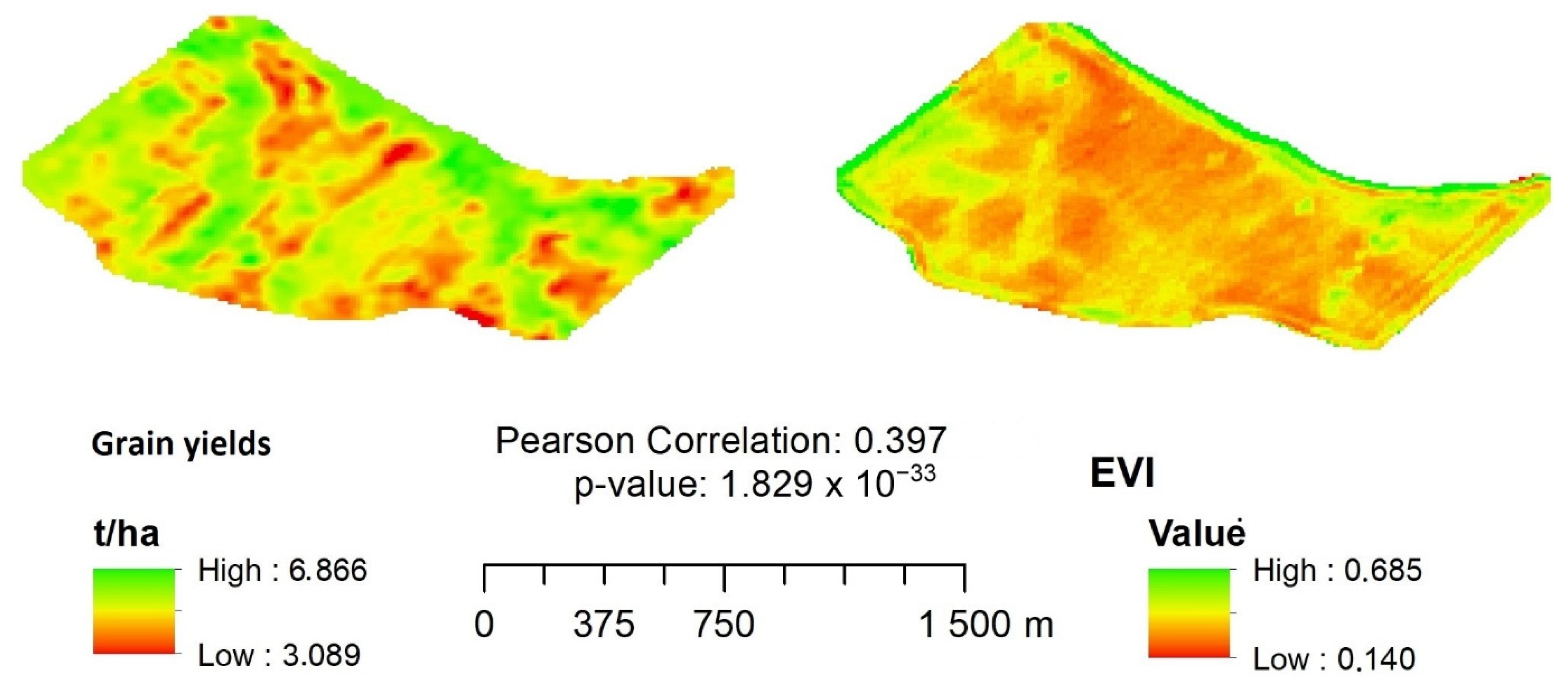
Evaluation of EVI and NDVI indices on selected soil blocks where wheat was grown, and comparison of these with yield maps.

(2)

Processing of EVI index for selected periods.

(3)

Identification of places with soil degradation and determination of degradation rate.

(4)

Correlation of degradation rate and EVI index.

(5)

Definition of highly degradation-affected localities (erosional areas) and depositional areas.

(6)

Simple statistics of the EVI index within the category of erosional and depositional areas were performed, and general information on the percentage decrease in yield was obtained.

Google Earth Explorer (GEE) mapping services were used to calculate remote sensing indexes through the R rgee library, which converts all R commands to GEE PythonAPI commands.

The assessment of sites affected by soil degradation was based on several approaches. The first was the use of the classical empirical USLE model with a variant of multiple flow direction calculation using the TAUDEM tool, which provides a more accurate distribution of erosion surfaces than the use of the standard single flow direction. ArcGIS 10.4 GIS software was used for the calculation and its specific extension developed by authors within the research for the needs of erosion modelling.

However, by simple visual comparison of the defined erosion areas and the yield model, it was clear that this model was not of much use for comparison. It captures only the manifestation of erosion in a given place, not accumulation.

Therefore, the USPED erosion-deposition model was subsequently used, which makes it possible to quantify both the rate of erosion and deposition of soil on a given plot.

However, the disadvantage of erosion-deposition models is the fact that they are based only on the morphology of the terrain and do not consider the possible influence of agricultural activity.

Therefore, another approach was considered, based on image analysis of remote sensing images at a time when there was bare ground in the given localities. However, even this approach is not entirely the most suitable for automatic processing, as it is difficult to determine the period when there was bare ground on a given block. These “time windows” are individual.

The authors of the article were therefore inspired by the work of Demattê et al. [51] and used a similar approach using only remote sensing data from the Sentinel-2 MSI: MultiSpectral Instrument, Level-1C satellite with a resolution accuracy of 10 m.

The schematic procedure for determining the time windows when the land was bare was based on a collection of images from the period at the beginning of sensing by the SENTINEL-2 satellite (2015) to the present. All images that meet the following conditions have been filtered from this collection:

Cloudy_pixel_percentage < 10%

Normalized Difference Vegetation Index (NDVI) < 0.35

Normalized Burned Ratio (NBR) < 0.1

where

$$\mathrm{NDVI}=\frac{\mathrm{B}8-\mathrm{B}4}{\mathrm{B}8+\mathrm{B}4}, \mathrm{NBR}=\frac{\mathrm{B}8-\mathrm{B}12}{\mathrm{B}8+\mathrm{B}12}$$

NBR is generally used for highlighting areas with damages by fires, while Normalized Difference Vegetation Index (NDVI) quantifies vegetation by measuring the difference between near-infrared (which vegetation strongly reflects) and red light (which vegetation absorbs).

Furthermore, pixels with cloud or shadows of cloud were filtered by means of QA60 cloud mask band.

The resulting bands B4, B3, and B2 were averaged to create the index I_deg = (B4 + B3 + B2)/3. The panchromatic map produced in this way creates structures of light and dark areas that correlate almost exactly with much more accurate aircraft images in places where bare ground is captured.

Pearson’s correlation was used for the resulting correlation and estimation of statistical significance, where 10% of the total area (number of pixels) of the processed soil block was selected as a statistical sample.

To gain information on how much the depositional areas of the slope differ from erosional areas, the field was divided into three categories: apart from areas with high erosion and high deposition, the rest were transient areas. This division was based on the 33rd and 66th percentiles of the Id index, where pixel values greater than the 66th percentile were considered erosion zones; pixel values lower than the 33rd percentile were considered depositional zones.

Subsequently, the average values of the EVI index were obtained from these erosional/depositional areas. In this way, the rate of decrease in EVI index, representing crop yield, was calculated.

3. Results

In the area of interest (Figure 1), a survey of selected physical, chemical, and biochemical properties was carried out. Many statistically significant differences were demonstrated, which indicate changes in soil properties in erosional and depositional areas (

Table 1. Basic statistical evaluation (average values) of soil properties, including a two-sample t-test for differentiation of erosional and depositional areas. Statistically significant results are marked by red.

Variable	t-Tests
	Mean—Erosional Parts	Std.Dev.	Mean—Depositional Parts	Std.Dev.	t-Value	p
pH/H2O	7.81	0.10	7.67	0.19	2.76	0.009
pH/CaCl2	7.65	0.12	7.55	0.17	2.06	0.047
Ca (mg/kg)	8694.00	1081.45	6660.61	1230.10	5.27	0.000
K (mg/kg)	163.17	47.95	236.17	88.95	−3.06	0.004
Mg (mg/kg)	296.28	42.34	283.44	37.41	0.96	0.342
P (mg/kg)	41.00	19.42	61.33	25.17	−2.71	0.010
Corg. (%)	2.10	0.21	2.22	0.39	−1.09	0.285
Ntot. (%)	0.13	0.02	0.17	0.02	−4.32	0.000
C:N	16.16	2.24	13.25	1.94	4.17	0.000
C CHL (%)	0.29	0.10	0.48	0.16	−4.26	0.000
C HK (%)	0.12	0.07	0.26	0.10	−5.13	0.000
C FK	0.16	0.05	0.21	0.08	−2.31	0.027
HK/FK	0.77	0.35	1.26	0.42	−3.85	0.000
Cellulase act. (μg GE/g DW/24 h)	104.08	50.69	103.79	30.47	0.02	0.984
Urease act. (μg N/g DW/2 h)	778.39	309.83	952.02	344.68	−1.59	0.121
Dehydrogen. act. (μg TPF/g DW/16 h)	2.89	1.20	4.16	1.98	−2.32	0.026
Acid phosph. act. (μg NP/g DW/h)	153.13	42.99	190.53	40.49	−2.69	0.011

).

By using an Ag Leader yield meter installed on the combine harvester, yield data were obtained and subsequently correlated with the EVI values from the period from 1st to 30th April of the same year (2018). The results obtained (Figure 2) show a moderately strong Pearson correlation r = 0.398. The correlation is statistically significant with p-value = 1.8 × 10⁻³³.

On blocks where no data from the yield meter were available, the EVI index was used as a representative of yield values to determine the relationship between degradation-endangered areas and yield.

Areas of land were selected, on a total of seven blocks, where winter wheat was grown in the period 2016–2019 (Figure 1).

To define heavily erosion-affected areas of land, the authors applied a slightly modified method according to Demattê et al. [35] (see Methods). This allowed erosion manifestation on chernozem soils to be captured by identifying visibly lighter areas. Figure 3 and Figure 4 show an example of the output of degraded areas based on remote sensing, in comparison with an orthophoto image of the same area (part of the area of interest in the vicinity of the village of Čejkovice). Despite the much lower resolution of the remote sensing image (1 px = 10 m) compared to aerial photographs, the results relatively accurately copy the visible erosion structures evident in the orthophoto and extend them by erosional areas that are less visible or hidden in the orthophoto due to the current vegetation.

Individual plots during individual periods were subsequently processed in the manner shown in Figure 5. A 10% sample of randomly selected pixels from the plot was used to obtain a Pearson correlation between Id (degradation) and EVI. Subsequently, the land was reclassified, based on the 33rd and 66th percentiles of the degradation threat index, into three categories—highly depositional, highly erosional, and transitional area. The average EVI value was then found on the highly depositional and erosional areas, and subsequently also the ratio of these values, which indirectly quantifies yield loss on degraded soil.

Table 2. Correlation of erosional areas determined on the basis of remote sensing and EVI values, supplemented by the ratio of the average EVI value.

Year	Field Block	p-Value	Pearson Correlation	EVI_Rate_Acc_Ero
2016 **	1601/16	1.8 × 10−14	0.27	0.881
2016 ***	8602/8	7.6 × 10−1	−0.02	0.957
2016 *	9801/2	2.2 × 10−7	−0.25	1.085
2016 *	5501/11	7.9 × 10−3	−0.09	1.027
2017 *	0701/15	1.5 × 10−5	−0.17	1.183
2017 *	1601/16	3.2 × 10−5	−0.16	0.918
2017 *	6904/1	4.0 × 10−22	−0.29	1.213
2017 *	5501/11	2.7 × 10−15	−0.27	1.208
2018 *	8602/8	8.6 × 10−11	−0.42	1.254
2018 *	6904/1	7.3 × 10−4	−0.15	1.091
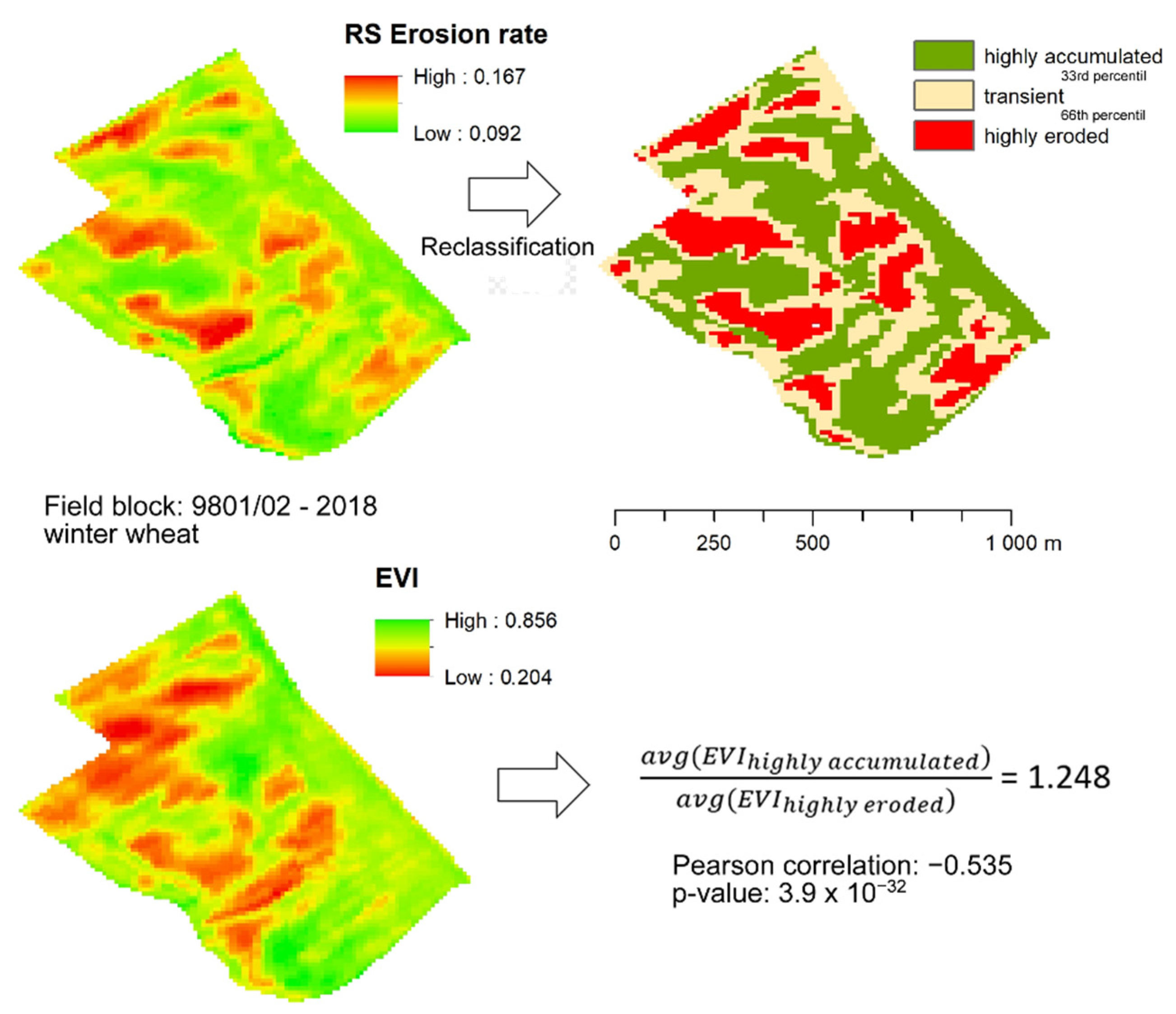
2018 *	9801/2	3.9 × 10−32	−0.53	1.249
2018 *	9803/1	3.1 × 10−11	−0.33	1.231
2018 *	0701/15	2.0 × 10−2	−0.08	1.224
2019 *	6904/1	1.4 × 10−55	−0.45	1.289
2019 *	8602/8	1.9 × 10−14	−0.37	1.084
2019 ***	1601/16	4.4 × 10−1	−0.03	1.062

* statistically significant negative correlation between EVI and erosion. ** statistically significant positive correlation between EVI and erosion. *** without significant correlation.

shows all correlation results and yield comparisons on highly erosional and highly depositional areas. The negative correlation confirms the assumption that yield is lower on eroded soil. This negative correlation was found in 15 locations out of 16; in 14 cases the correlation was statistically significant.

If we consider only statistically significant results, with the expected decrease in yield on degraded areas (14 plots out of 16), we can obtain an approximate weighted rate between yield on defined depositional and degraded areas, which for our area of interest comes to/equates to 16 ± 1 percent.

4. Discussion

Locations were chosen in the chernozem-soil, erosion-endangered region of South Moravia. In this area, we initially surveyed selected physical, chemical, and biochemical properties of soil in erosional and depositional areas (Table 1). The results from these investigated locations correspond to the conclusions for a larger area of South Moravia [52,53] and show differences between the studied erosional and depositional areas in many characteristics. Regarding chemical properties, our results also agree with the conclusions of other authors (e.g., [54,55,56]), with several characteristics showing statistically significant higher values in depositional areas compared to erosional areas. Thus, in some cases, the values are higher, but not statistically significant. Lower values in the depositional parts of the slope were recorded for Ca and the related pH/H₂O and pH/CaCl₂, which indicates intensive erosion processes and the occurrence of calcareous loess near the soil surface. This is consistent with the results of Hammerová et al. [57]. The activity of soil enzymes was statistically significantly higher for dehydrogenase and acid phosphatase, for other enzymes the activities were higher in the deposition area, but they were not statistically significant. Higher activity in deposition areas also corresponds to other studies (e.g., [58,59]). Physical characteristics (texture, bulk density, porosity) were monitored in the study areas, and values between erosional and depositional areas also differed, but not statistically significantly. With regard to fine fractions, this may be due to the loss of these fine particles during off-site erosion processes [60]. After a survey of the basic soil characteristics, it can be stated that there are differences between the erosional and depositional parts of the slope.

The correlation of certain remote sensing indices with crop yield is described in many studies (e.g., [30,33,61]). With regard to this, in our research we used the often cited Enhanced Vegetation Index (EVI). It is not always possible to obtain yield maps of the territory, which would certainly be a more accurate basis for our purpose, because in normal agricultural operation they are not ascertained on the scale of individual plots. Therefore, in places where yield maps are unavailable, we used the generally accepted correlate of crop yield in the form of the EVI. The EVI was selected in terms of explanatory power and applicability in practice. Nevertheless, the aforementioned studies, relating the EVI to yield characteristics, concern other locations. For verification in our sites as well, we selected soil blocks on land where yield had been determined by precision agriculture. The results (Figure 2) confirm the facts found in the cited literature that the EVI could also be used in our conditions.

Defining sites with some degree of soil degradation was more complicated. Although there are erosion and erosion-deposition models that are based on the morphology of terrain and allow the rate of erosion and deposition to be quantified [62], their use proved to be unsuitable for our needs. Although the USLE erosion model, correctly defines erosional areas, especially in the vicinity of valleys, it is in these places that considerable deposition of material occurs, and thus higher yield, which the model was unable to take into account. Deposition data were also necessary for comparison, so we could rule out simple erosion models. As an erosion-deposition model, we chose the USPED model [63], which is based on the USLE model and essentially defines and quantifies erosional and depositional areas based on terrain morphology. Each model has its specifics and, in the case of morphologically complex sites typical of our selected areas, the USPED modelhas certain inaccuracies in the form of alternating pixels representingdeposition and erosion with high intensity. Although visual comparison with orthophotos, in which soil degradation is evident, shows apparently similar structures, where lower values of EVI index and thus indirectly yields are visible on degraded areas, statistical evaluation in terms of random selection of individual pixels and their mutual comparison does not correspond. Statistically significant differences were not apparent until areas were generalized into two categories—erosional areas and depositional areas, with a threshold determined by the median of all values.

We were therefore looking for a way to use visible and typically colored patterns of degradation, on chernozem soils, in detailed orthophoto maps. These maps are usually not available in the amount required or at the appropriate time to provide this information for all the plots studied. The use of remote sensing is an alternative, but in practice there is often a problem of finding suitable images unaffected by atmospheric influences during the necessarily short time period. The solution was to use the method described by Demattê et al. [35], where the authors try to define bare soils on a much larger scale, on which certain spatial structures are visible, which can correlate with the amount of humus. The solution described by the authors is designed for LANDSAT satellites with a spatial resolution of 30 m. In terms of accuracy, we modified the method for the higher resolution of the SENTINEL-2 satellite (10 m) in the hope that the resulting spatial structure would then correspond to the actual degradation manifestations observed in orthophotos.

This assumption was fulfilled, so this was the way of specifying the degraded areas.

Subsequent results showed that most of the studied plots under conventional management confirmed the fact that erosion-endangered soils show lower biomass production than non-endangered soils. In one case, the correlation was not proven; in another, it was even negative, which we attribute to the influence of specific management in plant nutrition and soil compaction at the edge of the plot.

Definition of highly erosive or highly depositional areas is to some extent subjective. For our purposes we have chosen the percentile method for evaluation, but other methods, such as expert estimation, can be used. In some cases, where erosional and depositional areas are not very visible in localities, this division may not be entirely meaningful. However, in our region, with chernozems and complex terrain morphology, these areas were easily distinguishable. The average area-weighted value of the ratio of EVI index on depositional and erosional areas is based on approx. 1.16 + −0.1, which corresponds to 16% higher yield on non-degraded, or depositional areas compared to degraded ones. These fit the results of further research, although it should be emphasized that published results comparing yield on various erosion-prone sites show wide variability due to the use of flawed methodology [18].

Research results often vary, depending on the specific natural and economic conditions of the habitat and the intensity of erosion. On chernozems, erosion was studied by Gu et al. [64], who state that to maintain productivity, it is necessary to preserve the black soil layer, which is significantly disturbed in our study areas and then affects the level of yield. Soil erosion can lead to intensive transport of soil particles, sediment deposition, and loss of SOM, all of which limit agricultural productivity. Soil erosion not only redistributes SOC in the landscape, but has a broader effect on soil function and ecosystem sustainability [65]. Surface horizons tend to be rich in SOM, and erosion then changes soil properties and reduces soil quality. This soil quality deterioration reduces soil productivity and crop yield [13,19,66,67]. Over a 16-year experiment on chernozem soils, Larney et al. [27] describe grain yield reduction ranging from 10% to almost 40% with 5 to 20 cm soil removal, with greater dryland loss compared to irrigated land. Papiernik et al. [68] describe erosional areas with calcareous material on the surface and reduction in wheat yield of 50% and more. On the other hand, higher yield was recorded in the deposition parts of slopes. This is described, for example, by Cox et al., Kravchenko et al., and Stewart et al. [69,70,71]. Currently, the evaluation of horizontal contrast between areas with different degrees of erosion is an important issue in terms of evaluating the effect of erosion on soil productivity. In this context, for example, Bakker et al. [18] describe an average reduction in crop productivity of 4.3% per 10 cm of eroded soil using comparative-plot methods, 10.9% using transect methods, and 26.6% using desurfacing experiments. Schumacher et al. [72] describe a 7% yield reduction comparing soil thicknesses of 0.75 m and 0.59 m in north-central US conditions. Published experiments in the US prairie region show a 50% wheat yield on eroded soils compared to uneroded or depositional sites [68]. Lower values are reported by Panagos et al. [4], who document that on around 12 million hectares of European agricultural land, which suffers from severe erosion, about 0.43% of crop productivity is lost annually, which is about 1.25 billion euro per year. Our results, from the strongly erosion-endangered soils in our study, show higher values in the observed winter wheat, and tend to fall within the limits stated by the afore-mentioned authors (e.g., [18,27]).

5. Conclusions

In our research, we focused on identifying differences in crop production in erosional and depositional areas, over larger areas and over a longer period of time. For this purpose, we decided to use remote sensing tools, both to identify degraded areas and also to obtain EVI values for the monitored land, which according to our verification correlate well with actual crop yield. We decided to identify degraded areas by means of remote sensing, given that the commonly used USLE or USPED models did not correspond to yield characteristics, especially near valleys, where greater erosion and deposition of soil occurs, to which the model (USLE) responded by alternating erosional and depositional areas in line structures, which did not correspond to reality. Moreover, the disadvantage of using these models is the morphology of the terrain, where they do not take into account the current state, which could change due to farming practices. The proposed method of identification of degraded areas by remote sensing can be used on chernozem soils, but as it does not use only indices of the visible spectrum, it has the potential of being applied to other soils where erosion is not visible. This will be the subject of further research.

The proposed procedure for analyzing the relationship between crop yield and soil degradation is certainly not the only one possible. However, its simplicity means it can quickly evaluate large areas without the need for more spatial data. Its applicability outside chernozem areas will also be the subject of further research, as well as the question of the influence of differentiated plant nutrition (e.g., in precision agriculture) on yield characteristics depending on the intensity of erosion or deposition of material.

The presented research specified the effects of erosion on production in the chernozem area of South Moravia. Its outputs concerning production and economics are discussed with farmers and policymakers in terms of designing optimal anti-erosion measures to protect soil, water resources, and sustainable production for farmers.

References

- Amundson, R.; Berhe, A.A.; Hopmans, J.W.; Olson, C.; Sztein, A.E.; Sparks, D.L. Soil and human security in the 21th century. Science 2015, 348, 1261071. [Google Scholar] [CrossRef] [PubMed] [Green Version]
- Pimentel, D.; Harvey, C.; Resosudarmo, P.; Sinclair, K.; Kurz, D.; Mcnair, M.; Crist, S.; Shpritz, L.; Fitton, L.; Saffouri, R.; et al. Environmental and economic costs of soil erosion andconservation benefits. Science 1995, 267, 1117–1123. [Google Scholar] [CrossRef] [PubMed] [Green Version]
- van den Born, G.J.; de Haan, B.J.; Pearce, D.W.; Howarth, A. Technical Report on Soil Degradation in Europe: An Integralted Economic and Environmental Assessment; RIVM Report 481505018; National Institute of Public Health and Environment—RIVM: Bilthoven, The Netherlands, 2000. [Google Scholar]
- Panagos, P.; Standardi, G.; Borrelli, P.; Lugato, E.; Montanarella, L.; Bosello, F. Cost of agricultural productivity loss due to soil erosion in the European Union: From direct cost evaluation approaches to the use of macroeconomic models. Land Degrad. Dev. 2018, 29, 471–484. [Google Scholar] [CrossRef]
- Nkonya, E.; Anderson, W.; Kato, E.; Koo, J.; Mirzabaev, A.; von Braun, J.; Meyer, S. Global Cost of Land Degradation. In Economics of Land Degradation and Improvement—A Global Assessment for Sustainable Development; Nkonya, E., Mirzabaev, A., von Braun, J., Eds.; Springer International Publishing: Cham, Switzerland, 2016; pp. 117–165. [Google Scholar]
- Sartori, M.; Philippidis, G.; Ferrari, E.; Borrelli, P.; Lugato, E.; Montanarella, L.; Panagos, P. A linkage between the biophysical and the economic: Assessing the global market impacts of soil erosion. Land Use Pol. 2019, 86, 299–312. [Google Scholar] [CrossRef]
- Kosmas, C.; Danalatos, N.G.; López-Bermúdez, F.; Romero-Díaz, M.A. The Effect of Land Use on Soil Erosion and Land Degradation under Mediterraneanconditions. In Mediterranean Desertification: A Mosaic of Processes and Responses; Thornes, J.B., Ed.; John Wiley & Sons: Chichester, UK, 2002; p. 518. [Google Scholar]
- García-Ruiz, J.M. The effects of land uses on soil erosion in Spain: A review. Catena 2010, 81, 1–11. [Google Scholar] [CrossRef]
- Panagos, P.; Borrelli, P.; Robinson, D.A. Common agricultural policy: Tackling soil loss across Europe. Nature 2015, 526, 195. [Google Scholar] [CrossRef] [PubMed]
- Borrelli, P.; Panagos, P.; Märker, M.; Modugno, M.; Schütt, B. Assessment of the impacts of clear cutting on soil loss by water erosion in Italian forests: First comprehensive monitoring and modelling approach. Catena 2017, 149, 770–781. [Google Scholar] [CrossRef]
- Colombo, S.; Hanley, N.; Calatrava-Requena, J. Designing policy for reducing the off-farm effects of soil erosion using choice experiments. J. Agric. Econ. 2005, 56, 81–95. [Google Scholar] [CrossRef]
- Telles, T.S.; de Fátima, G.M.; Dechen, S.C.F. The costs of soil erosion [Os custos da erosão do solo]. Rev. Bras. Cienc. Solo 2011, 35, 287–298. [Google Scholar] [CrossRef]
- Tengberg, A.; Da Veiga, M.; Dechen, S.C.F.; Stocking, M. Modelling the impact of erosion of soil productivity: A comparative evaluation of approaches on data from Southern Brazil. Exp. Agric. 1998, 34, 55–71. [Google Scholar] [CrossRef]
- Martínez-Casasnovas, J.A.; Ramos, M.C. The cost of soil erosion in vineyard fields in the Penedes–Anoia Region (NE Spain). Catena 2006, 68, 194–199. [Google Scholar] [CrossRef]
- Bakker, M.M.; Govers, G.; Jones, R.A.; Rounsevell, M.D.A. The Effect of Soil Erosion on Europe’s Crop Yields. Ecosystems 2007, 10, 1209–1219. [Google Scholar] [CrossRef] [Green Version]
- de la Rosa, D.; Moreno, J.A.; Mayol, F.; Bonsón, T. Assessment of soil erosion vulnerability in western Europe and potential impact on crop productivity due to loss of soil depth using ImpelERO model. Agric. Ecosyst. Environ. 2000, 81, 179–190. [Google Scholar] [CrossRef]
- García-Ruiz, J.M.; Beguería, S.; Lana-Renault, N.; Nadal-Romero, E.; Cerdà, A. Ongoing and emerging questions in water erosion studies. Land Degrad. Dev. 2017, 28, 5–21. [Google Scholar] [CrossRef]
- Bakker, M.M.; Govers, G.; Rounsevell, M.D.A. The crop productivity–erosion relationship: An analysis based on experi-mental work. Catena 2004, 57, 55–76. [Google Scholar] [CrossRef]
- Den Biggelaar, C.; Lal, R.; Wiebe, K.; Breneman, V. The global impact of soil erosion on productivity I: Absolute and relative erosion induced yield losses. Adv. Agron. 2003, 81, 1–48. [Google Scholar]
- Den Biggelaar, C.; Lal, R.; Wiebe, K.; Breneman, V. The impact of soil erosion on crop yield in North America. Adv. Agron. 2001, 72, 1–52. [Google Scholar]
- Quinton, J.N.; Govers, G.; Van Oost, K.; Bardgett, R.D. The impact of agricultural soil erosion on biogeochemical cycling. Nat. Geosci. 2010, 3, 311–314. [Google Scholar] [CrossRef] [Green Version]
- Herbrich, M.; Gerke, H.H.; Sommer, M. Root development of winter wheat on erosion-affected soils depending on the position in a hummocky ground moraine soil landscape. J. Plant Nutr. Soil Sci. 2018, 181, 147–157. [Google Scholar] [CrossRef]
- Trimble, S.W.; Crosson, P.R. U.S. Soil erosion rates—Myth and reality. Science 2000, 289, 248–250. [Google Scholar] [CrossRef] [Green Version]
- Yaalon, D.H.; Arnold, R.W. Attitudes toward soils and their societal relevance: Then and now. Soil Sci. 2000, 165, 5–12. [Google Scholar] [CrossRef]
- Robinson, D.A.; Fraser, I.; Dominati, E.J.; Davísdóttir, B.; Jónsson, J.O.G.; Jones, L.; Jones, S.B.; Tuller, M.; Lebron, I.; Bristow, K.L.; et al. On the value of soil resources in the context of natural capital and ecosystem service delivery. Soil Sci. Soc. Am. J. 2014, 78, 685–700. [Google Scholar] [CrossRef] [Green Version]
- Gunatilake, H.M.; Vieth, G.R. Estimation of on-site cost of soil erosion: A comparison of replacement and productivity change methods. J. Soil Water Conserv. 2000, 55, 197–204. [Google Scholar]
- Larney, F.J.; Janzen, H.H.; Olson, B.M.; Olson, A.F. Erosion–productivity–soil amendment relationships for wheat over 16 years. Soil Tillage Res. 2009, 103, 73–83. [Google Scholar] [CrossRef]
- Posthumus, H.P.; Deeks, L.K.; Rickson, R.J.; Quinton, J.N. Costs and benefits of erosion control measures in the UK. Soil Use Manage. 2015, 31 (Suppl. S1), 16–33. [Google Scholar] [CrossRef]
- Bizoza, A.R.; de Graaff, J. Financial cost–benefit analysis of bench terraces in Rwanda. Land Degrad. Dev. 2012, 23, 103–115. [Google Scholar] [CrossRef]
- Kogan, F.; Salazar, L.; Roytman, L. Forecasting crop production using satellite-based vegetation health indices in Kansas, USA. Int. J. Remote Sens. 2012, 33, 2798–2814. [Google Scholar] [CrossRef]
- Zhang, J.; Feng, L.; Yao, F. Improved maize cultivated area estimation over a large scale combining MODIS–EVI time series data and crop phenological information. ISPRS J. Photogramm. Remote. Sens. 2014, 94, 102–113. [Google Scholar] [CrossRef]
- Huang, X.; Liu, J.; Zhu, W.; Atzberger, C.; Liu, Q. The optimal threshold and vegetation index time series for retrieving crop phenology based on a modified dynamic threshold method. Remote Sens. 2019, 11, 2725. [Google Scholar] [CrossRef] [Green Version]
- Liu, J.; Huffman, T.; Qian, B.; Shang, J.; Li, Q.; Dong, T.; Davidson, A.; Jing, Q. Crop Yield Estimation in the Canadian Prairies Using Terra/MODIS-Derived Crop Metrics. IEEE J. Sel. Top. Appl. Earth Observ. Remote Sens. 2020, 13, 2685–2697. [Google Scholar] [CrossRef]
- Seo, B.; Jihye, L.; Kyung-Do, L.; Sukyoung, H.; Sinkyu, K. Improving remotely sensed crop monitoring by NDVI-based crop phenology estimators for corn and soybeans in Iowa and Illinois, USA. Field Crop. Res. 2019, 238, 113–128. [Google Scholar] [CrossRef]
- Demattê, J.A.M.; Fongaro, C.T.; Rizzo, R.; Safanelli, J.L. Geospatial Soil Sensing System (GEOS3): A powerful data mining procedure to retrieve soil spectral reflectance from satellite images. Remote. Sens. Environ. 2018, 212, 161–175. [Google Scholar] [CrossRef]
- Netopil, P.; Šarapatka, B.; Ayalew, D.A.; Drncová, K. Multi-temporal analysis of erosional plots using aerial images and deep soil probes. Phys. Geogr. 2021. [Google Scholar] [CrossRef]
- Hein, L. Assessing the costs of land degradation: A case study for the Puentes catchment, southeast Spain. Land Degrad. Dev. 2007, 18, 631–642. [Google Scholar] [CrossRef]
- IUSS Working Group WRB. World Reference Base for Soil Resources 2014; Updated 2015; World Soil Resources Report No. 106; Food and Agriculture Organization: Rome, Italy, 2015. [Google Scholar]
- Zbíral, J.; Honsa, I. (Eds.) Methods of Soil Analysis. Part I. (in Czech); Central Institute for Supervising and Testing in Agriculture: Brno, Czech Republic, 2010. [Google Scholar]
- Kandeler, E.; Palli, E.; Stemmer, M.; Gerzabek, M.H. Tillage changes microbial biomass and enzymes activities in particle size fractions of a Haplic Chernozem. Soil Biol. Biochem. 1999, 31, 1253–1264. [Google Scholar] [CrossRef]
- Mehlich, A. Mehlich no. 3 soil test extractant: A modification of Mehlich no. 2. Commun. Soil Sci. Plant Anal. 1984, 15, 1409–1416. [Google Scholar] [CrossRef]
- International Organization for Standardization. Soil Quality—Determination of Organic Carbon in Soil by Sulfochromic Oxidation; ISO 14235; International Organization for Standardization: Geneva, Switzerland, 1998. [Google Scholar]
- Zbíral, J.; Malý, S.; Váňa, M. (Eds.) Methods of Soil Analysis. Part III. (in Czech); Central Institute for Supervising and Testing in Agriculture: Brno, Czech Republic, 2011. [Google Scholar]
- International Organization for Standardization. Soil Quality—Determination of Nitrogen—Modified Kjeldahl Method; ISO 11261; International Organization for Standardization: Geneva, Switzerland, 1995. [Google Scholar]
- International Organization for Standardization. Soil Quality—Determination of Ph; ISO 10390; International Organization for Standardization: Geneva, Switzerland, 2000. [Google Scholar]
- Kononova, M.M.; Bělčiková, N.P. A rapid analysis of humus composition in mineral soil. Pochvovedenie 1961, 10, 75–87. (In Russian) [Google Scholar]
- Schinner, F.; von Mersi, W. Xylanase, CM-cellulase and invertase activity in soil: An improved method. Soil Biol. Biochem. 1990, 22, 511–515. [Google Scholar] [CrossRef]
- Tabatabai, M.A.; Bremner, J.M. Use of p-nitrophenyl phosphate for assay of soil phosphatase activity. Soil Biol. Biochem. 1969, 1, 301–307. [Google Scholar] [CrossRef]
- Ross, D.J. Effects of storage on deydrogenase activities of soil. Soil Biol. Biochem. 1970, 2, 55–61. [Google Scholar] [CrossRef]
- Tabatabai, M.A.; Bremner, J.M. Assay of urease activity in soils. Soil Biol. Biochem. 1972, 4, 479–487. [Google Scholar] [CrossRef]
- Demattê, J.A.M.; Guimarães, C.C.B.; Fongaro, C.T.; Vidoy, E.L.F.; Sayão, V.M.; Dotto, A.C.; Santos, N.V. Satellite Spectral Data on the Quantification of Soil Particle Size from Different Geographic Regions. Rev. Bras. Cienc. Solo 2018, 42, 1–14. [Google Scholar] [CrossRef]
- Šarapatka, B.; Čáp, L.; Bílá, P. The varying effect of water erosion on chemical and biochemical soil properties in different parts of Chernozem slopes. Geoderma 2018, 314, 20–26. [Google Scholar] [CrossRef]
- Bílá, P.; Šarapatka, B.; Horňák, O.; Novotná, J.; Brtnický, M. Which quality indicators reflect the most sensitive changes in the soil properties of the surface horizons affected by the erosion processes? Soil Water Res. 2020, 15, 116–124. [Google Scholar] [CrossRef]
- Papiernik, S.K.; Lindstrom, M.J.; Schumacher, T.E.; Schumacher, J.A.; Malo, D.D.; Lobb, D.A. Characterization of soil profiles in a landscape affected by long term tillage. Soil Tillage Res. 2007, 93, 335–345. [Google Scholar] [CrossRef]
- Nie, X.J.; Zhao, T.Q.; Qiao, X.N. Impacts of soil erosion on organic carbon and nutrient dynamic in an alpine grassland soil. Soil Sci. Plant Nutr. 2013, 59, 660–668. [Google Scholar] [CrossRef] [Green Version]
- Liu, X.; Herbert, S.J.; Hashemi, A.M.; Zhang, X.; Ding, G. Effects of agricultural management on soil organic matter and carbon transformation—A review. Plant Soil Environ. 2006, 52, 531–543. [Google Scholar] [CrossRef] [Green Version]
- Hammerová, H.; Jandák, J.; Hrabovská, B.; Šimečková, J. The detailed characterization of land treatened by water erosion with soil type chernozem on loess at Dambořice. Mendelnet 2014, 250–254. Available online: https://mnet.mendelu.cz/mendelnet2014/articles/52_hammerova_1058.pdf?id=1058&file=52_hammerova_1058.pdf (accessed on 1 November 2021).
- Wicklings, K.; Grandy, S.A.; Kravchenko, A.N. Going with theflow: Landscape position drives differences in microbial biomass and activity in conventional, low input, and organic agricultural systems in the Midwestern U.S. Agric. Ecosyst. Environ. 2016, 218, 1–10. [Google Scholar] [CrossRef]
- Li, Z.; Xiao, H.; Tang, Z.; Huang, J.; Nie, X.; Huang, B.; Ma, W.; Lu, Y.; Zeng, G. Microbial responses to erosion-induced soil physico-chemical property changes in the hilly red soil region of southern China. Eur. J. Soil Biol. 2015, 71, 37–44. [Google Scholar] [CrossRef]
- Stone, J.R.; Gilliam, J.W.; Cassel, D.K.; Daniels, R.B.; Nelson, L.A.; Kieiss, H.J. Effects of erosion and landscape position on the productivity of Piedmont soils. Soil Sci. Soc. Am. J. 1985, 49, 987–991. [Google Scholar] [CrossRef]
- Vallentin, C.; Harfenmeister, K.; Itzerott, S.; Kleinschmit, B.; Conrad, C.; Spengler, D. Suitability of satellite remote sensing data for yield estimation in northeast Germany. Precis. Agric. 2021, 1–31. [Google Scholar] [CrossRef]
- Efthimiou, N.; Lykoudi, E.; Karavitis, C. Comparative analysis of sediment yield estimations using different empirical soil erosion models. Hydrol. Sci. J. 2017, 62, 2674–2694. [Google Scholar] [CrossRef]
- Pistocchi, A.; Cassani, G.; Zani, O. Use of the USPED Model for Mapping Soil Erosion and Managing Best Land Conservation Practices. In Proceedings of the First Biennial Meeting of the International Environmental Modelling and Software Society on Integrated Assessment and Decision Support, Lugano, Switzerland, 24–27 June 2002; Volume 3, pp. 163–168. Available online: http://www.iemss.org/iemss2002/ (accessed on 1 November 2021).
- Gu, Z.; Xie, Y.; Gao, Y.; Ren, X.; Cheng, C.; Wang, S. Quantitative assessment of soil productivity and predicted impacts ofwater erosion in the black soil region of northeastern China. Sci. Total Environ. 2018, 637–638, 706–716. [Google Scholar] [CrossRef] [PubMed]
- Olson, K.R.; Al-Kaisi, M.; Lal, R.; Cihacek, L. Soil organic carbon dynamics in eroding and depositional landscapes. Open J. Soil Sci. 2016, 6, 121. [Google Scholar] [CrossRef] [Green Version]
- Verity, G.E.; Anderson, D.W. Soil erosion effects on soil quality and yield. Can. J. Soil Sci. 1990, 70, 471–484. [Google Scholar] [CrossRef] [Green Version]
- Duan, X.W.; Xie, Y.; Ou, T.H.; Lu, H.M. Effects of soil erosion on long-term soil productivity in the black soil region of northeastern China. Catena 2011, 87, 268–275. [Google Scholar] [CrossRef]
- Papiernik, S.K.; Lindstrom, M.J.; Schumacher, J.A.; Farenhorst, A.; Stephens, K.D.; Schumacher, T.E.; Lobb, D.A. Variation in soil properties and crop yield across an eroded prairie landscape. J. Soil Water Conserv. 2005, 60, 388–395. [Google Scholar]
- Cox, M.S.; Gerard, P.D.; Wardlaw, M.C.; Abshire, M.J. Variability of selected soil properties and their relationships with soybean yield. Soil Sci. Soc. Am. J. 2003, 67, 1296–1302. [Google Scholar] [CrossRef]
- Kravchenko, A.N.; Bullock, D.G.; Boast, C.W. Joint multifractal analysis of crop yield and terrain slope. Agron. J. 2000, 92, 1279–1290. [Google Scholar] [CrossRef] [Green Version]
- Stewart, C.M.; McBratney, A.B.; Skerritt, J.H. Site-specific durum wheat quality and its relationship to soil properties in a single field in Northern New South Wales. Precis. Agric. 2002, 3, 155–168. [Google Scholar] [CrossRef]
- Schumacher, T.E.; Lindstrom, M.J.; Mokma, D.L.; Nelson, W.W. Corn yield: Erosion relationships of representative loess andtill soils in the North-Central United States. J. Soil Water Conserv. 1994, 49, 77–81. [Google Scholar]