Article

Factor Analysis of Well Logs for Total Organic Carbon Estimation in Unconventional Reservoirs

1
Department of Geophysics, University of Miskolc, H-3515 Miskolc, Hungary
2
MTA-ME, Geoengineering Research Group, H-3515 Miskolc, Hungary
3
MOL Plc., Group E&P Subsurface and Field Development, H-5000 Szolnok, Hungary
*
Author to whom correspondence should be addressed.
Energies 2021, 14(18), 5978; https://doi.org/10.3390/en14185978
Submission received: 16 August 2021 / Revised: 10 September 2021 / Accepted: 16 September 2021 / Published: 20 September 2021
(This article belongs to the Special Issue Well Logging Applications)

Abstract

:
Several approaches have been applied for the evaluation of formation organic content. For further developments in the interpretation of organic richness, this research proposes a multivariate statistical method for exploring the interdependencies between the well logs and model parameters. A factor analysis-based approach is presented for the quantitative determination of total organic content of shale formations. Uncorrelated factors are extracted from well logging data using Jöreskog’s algorithm, and then the factor logs are correlated with estimated petrophysical properties. Whereas the first factor holds information on the amount of shaliness, the second is identified as an organic factor. The estimation method is applied both to synthetic and real datasets from different reservoir types and geologic basins, i.e., Derecske Trough in East Hungary (tight gas); Kingak formation in North Slope Alaska, United States of America (shale gas); and shale source rock formations in the Norwegian continental shelf. The estimated total organic content logs are verified by core data and/or results from other indirect estimation methods such as interval inversion, artificial neural networks and cluster analysis. The presented statistical method used for the interpretation of wireline logs offers an effective tool for the evaluation of organic matter content in unconventional reservoirs.

1. Introduction

The continuing demand for hydrocarbons, despite the overall decline in the industry due to the strongly emerging low-carbon advocacy, is evident in the further development of unconventional reservoirs. Several technologies and studies are being developed for further understanding of the distribution, accumulation patterns and resource evaluation of these complex reservoirs, among others. Unconventional reservoirs are such reservoirs from which the retrieval of hydrocarbons is commonly accomplished by methods beyond known traditional methods. These unconventional formations belong to those oil and gas resources for which industrial productivity is possible only by changing the rock permeability or fluid viscosity to alter the permeability–viscosity ratios [1]. In contrast, conventional resources are available for industrial production without the extra measures taken in the former. This general term is applied to such formations/techniques to differentiate them from conventional approaches.
These resources vary, including tight gas formations, shale gas, heavy oil, gas hydrates and coal bed methane tar sands [2]. Shale gas reservoirs as both source and reservoir for natural gas have a distinct response to well logs when compared to non-hydrocarbon-bearing source rocks [3]. This distinct response is due to the physical properties of the organic matter contained in these formations. The organic richness of these formations, expressed as total organic carbon (TOC in weight percent) content, and the clay volume are very important parameters for the evaluation of shale gas reservoirs. This study shows that these two parameters contribute majorly to the variances in the datasets. This is thus explored by employing the factor analysis technique to extract the underlying/latent variables for a quantitative description of the parameters.
The standard method for the determination of TOC involves the geochemical measurement of core samples (whole cores, cuttings or sidewall cores) in laboratories. However, the process involved in obtaining cores is expensive and time-consuming. Moreover, the millimeter-scale variability common in mudstone makes it very problematic to select multiple samples with the same attributes [4]. Thus, only a few samples collected at strategic intervals are analyzed. For huge shale formations, hence, information on the TOC is not continuous along with the interval. Moreover, the heterogeneous nature of these rocks, sampling errors and misses or destruction of samples may lead to inconsistencies in the analysis. An alternative to the geochemical processes lies therefore in the application of wireline logs with higher vertical resolution.
Furthermore, when using only open-hole wireline logs and geochemical measurements of core samples in linear approximations method (e.g., spectral gamma-ray, clay indicator and ΔlogR methods), some limitations and restrictions should be considered since some logs can be affected due to the natural characteristics of the well (e.g., specific lithology, complex mineralogy and type of fluid contained in pore space). For instance, the resistivity log plays an important role in TOC estimation (i.e., Passey’s method), although it is affected by many factors such as clay and pyrite volume and the bulk volume of water in the formation, and all these factors might be misleading during the TOC estimation applying methods based on resistivity logs. Additionally, the lack of enough data along the investigated interval makes the calibration procedure necessary to establish an accurate linear model difficult [5].
On the other hand, wireline logs have always played a major role in the determination of shale volume, which can also be confirmed by laboratory analysis. This is a very crucial step in the characterization of hydrocarbon reservoirs, especially as a lot of other important parameters are obtained from the estimated shale volume. A lot of these methods depend on the natural gamma-ray log, with more advanced methods employing the spectral gamma-ray log, which separates the thorium, uranium and potassium concentrations in their different energetic windows. Due to the evident observed well log responses of organic shale formations, various approaches have been developed for the estimation of organic richness and shale volume using wireline log data. This work is a further development in that regard.
By using the method of exploratory factor analysis, the underlying and unobserved relationships between the measured variables (e.g., well logs) are identified [6]. In this study, the factors are extracted from the input logs, and emphasis is placed on the first two factors for the estimation of shale volume and organic content. By application of the factor analysis technique, a strong assumption is made. As long as these well logs give distinct signatures or responses to the lithology and the organic content of the formations—for those unconventional resources/shale formations where the lithology and organic content are the predominantly controlling variables—a factor analysis model, as suggested in this work, will accord a higher explained variance to them. When the number of the extracted factors is greater than two, the nth extracted factor will have an explained variance with very little to meaningless contribution to the interpretation of the log data.
The simultaneous estimation of these two parameters as proposed in this study carries an advantage by increasing the overdetermination ratio so as to obtain reliable results. The described technique is shown as a reliable method, as it has been applied to both synthetic and real datasets from wells drilled into different geologic formations. The accuracy of the method is also compared to other evaluation methods for verification of the acquired results.

2. Materials and Methods

2.1. Geological Settings

The datasets analyzed for this study were obtained from different geological environments, Derecske Trough (Hungary), North Slope (AK, USA) and North Sea (Norway). This was necessary to test the feasibility of the proposed TOC evaluation method, as well as to identify its limitation(s). Moreover, while the first three datasets are described as belonging to an unconventional petroleum system, the Norwegian dataset originated from a source rock associated with a conventional petroleum system. The formations from which these wireline logs were obtained have all been identified as having potentials for oil/gas production.

2.1.1. Derecske Trough, Hungary

The interpretation from the synthetic/observed datasets was applied to a tight gas formation in Hungary, situated in the Neogene Pannonian Basin known as the Derecske Trough. The Middle Miocene sandstones and Upper Miocene formations are major plays of interest for tight gas exploration in Hungary. The Middle Miocene play corresponds to the Badenian sandstones that are located in depths greater than 3000 m. This play is formed mainly by sandstones with 6 to 10% porosity and low permeability; the source rocks are believed to be deep-water marine Middle Miocene shales, which mostly remain unexplored in the deepest part of the subbasins. However, where they have been explored, the Badenian shales have proved to be fair- to good-quality source rocks. The Upper Miocene play corresponds especially to the turbidites of Szolnok Formation, the major source rock of which is the underlying Endrőd Formation that is described as a highly overpressured Upper Miocene brackish-water shale. The zone of interest is a continuous basin-centered accumulation, with low porosity, between 5 and 8%, and low permeability, and is situated deep within the basin—reaching depths of over 3000 m. The TOC values in the play are generally low [7] but reach the requirements for unconventional reservoirs (>2% TOC). An extensive description of the geology of the Pannonian Basin and hydrocarbon exploration details of the investigated area can be read in [8].

2.1.2. North Slope, Alaska, USA

Alaska has two major oil and gas operations going on in the northern part of the state and the Cook inlet region in the southern part of the state. The analyzed well section is of the Jurassic to Lower Cretaceous Kingak formation (known as the K1 sequence) situated in the North Slope area. It is one of the three oil and gas source rock systems in the region. Lying at a burial depth of over 2700 m, the 300–380 m basal sequence is identified to be of marine and terrigenous origin, having organic matter from both sources and deposited in a marine siliciclastic setting during the opening of the Canadian basin [9,10].
The Kingak formation has been described as a dark-gray to dark-olive-gray shale and subordinate siltstone, claystone and clay ironstone [11]. The upper part is clay shale, silty shale and siltstone that have red, rusty-weathering ironstone beds. The lower section consists of a dark-gray to black fissile paper shale, dark-gray clay shale, minor claystone and beds and nodules of red-weathering ironstone [12]. The organic carbon content in the Kingak Shale formation varies from less than 0.6 to over 3.0 wt%. The thermal maturity of the formation presents a complex pattern that seems not to be related to the present-day depth of burial. The vitrine reflectance at a burial depth of 600 m is 0.5%, while it is 0.4% at depths of 3000 m [13].
A feasibility study of the factor analysis method was made using well logs of North Inigok 1 well drilled into the formation. The 90 m long interval analyzed in this study was earlier identified as a potential source rock using Passey’s method. The results obtained were verified using core data obtained from the section.

2.1.3. North Sea, Norway

Several datasets obtained from various wells drilled into geologic formations in the Norwegian continental shelf are also analyzed in this study. These are from prominent fields with established prospects for hydrocarbon production. Major potential source rocks in the region include the Farsund and Mandal shale formations. The formations are source rock beds linked to conventional reservoirs in the region. These black shale formations, equivalents of the Kimmeridge Clay, are very rich in organic materials and were deposited in the Jurassic.
The analyzed formation has been described with a varying thickness of tens of meters. It is formed by dark grey-brown to black, slightly calcareous to non-calcareous, carbonaceous claystone. It shows a very high level of radioactivity, as it contains a considerable amount of organic carbon content. Moreover, it is characterized by anomalously high resistivity and low velocity and density properties. Some stringers of limestone–dolomite and even sandstone can be found in some areas [14]. The organic richness of formations from one of such wells is discussed based on the results from the analysis carried out using the proposed method.

2.2. Traditional Determination of Organic Richness

Total organic carbon is the quantity of organic material deposited in a rock that can be converted into oil or gas, depending on the form of kerogen present. TOC in source rocks (and reservoir rocks as with shale gas reservoirs) can be determined analytically by established principles in geochemistry. While a few of the constraints with this method have been highlighted earlier, it is noteworthy to mention that it is the most accurate, and it is recommended that all TOC inferred from indirect well logging methods be calibrated to values measured using laboratory-based geochemical methods [15]. The need for the development of improved well logging methods is a result of high vertical variability in organic material in formations especially as a result of geologic and biotic conditions, as well as a complex function of many other interacting processes during deposition and burial [4]. To increase the vertical resolution of the estimated TOC, several wireline logging methods have been derived.
Diverse empirical (linear) well-log-based estimation methods have been developed to obtain an accurate TOC estimation; for instance, spectral gamma-ray log [16,17,18], bulk density log [19,20], clay indicator [21] and ΔlogR methods [22] are the best-known (empirical) techniques used nowadays. However, all these methods have their drawbacks; i.e., some limitations and restrictions should be taken into account since some logs can be affected due to the natural characteristics of the well (e.g., specific lithology, complex mineralogy and type of fluid contained in the pore space).
For instance, the resistivity log plays an important role in TOC estimation (i.e., Passey’s method), although it is affected by many factors such as clay and pyrite volume and the bulk volume of water in the formation, and all these factors might be misleading during the TOC estimation applying methods based on a limited number of well logs. Additionally, the lack of enough data along the investigated interval makes the calibration procedure needed to establish an accurate linear model difficult. Some studies have been conducted to analyze the importance of using different methods, such as statistical approaches, for estimating TOC content [5] since different petrophysical properties of the formation are considered in different well logs. For instance, the total and spectral gamma-ray logs commonly have an abnormally high response in highly organic-rich black shales that are potentially source rocks [17] due to the enrichment of uranium. Furthermore, the presence of organic matter can result in alteration of the formation resistivity, making such logs suitable to analyze the TOC, as in Passey’s method, since organic matter is usually nonconductive and highly increases the resistivity of the formation.
Porosity-based logs are used in Passey’s and clay indicator methods. These methods are based on the facts that organic matter or kerogen reduces the density of the rock due to its relatively low density and high acoustic transit times and that neutron records are affected by hydrogen in organic matter. Consequently, porosity will be overestimated using any of these logs [23]. Methods presently applied include the natural gamma spectroscopy method, which explores the relationship between uranium content and TOC to estimate the latter; the total gamma-ray intensity method; the bulk density method; and the ΔlogR method, which estimates TOC by overlapping porosity and resistivity [3,15,24].

2.3. Determination of TOC by Factor Analysis

Factor analysis is a multivariate statistical method that involves the reduction of a large dataset (several observed variables) to a relatively lesser number of factors (the latent variables) by finding the interrelationship between the observed variables. By reducing the dimension of variability, we are able to explore unobserved properties of the rock that are responsible for the observed well log responses. The latent factors, supposedly accounting for the intercorrelations of the response variables, should thus be uncorrelated after they are extracted from a large observed dataset [25,26,27].
The formulation of the statistical problem can be made by first creating an N-by-K matrix of the original data:
D = d 11 d 12 d 1 k d 1 K d 21 d 22 d 2 k d 2 K d n 1 d n 2 d nk d nK d N 1 d N 2 d Nk d NK ,
where N is the total number of data (depth) points and K is the number of logging data/response variables. For the given dataset D, if both observed variables and latent factors are measured in deviations from their means, it leads to the following factor analysis model:
D = F L T + E ,
where F is the N-by-a matrix of the extracted factors and LT is the transposed K-by-a matrix of the factor loadings (practically being the correlation coefficients between observed variables and latent factors), and E is the N-by-K matrix of residuals or unique part of the matrix D. The objective of the factor analysis method is the determination of the number of factors and estimation of the factor loadings that suitably explains the variables in the dataset. The factor analysis algorithm applied in this work is based on the Jöreskog solution [25], which gives a quick estimate of the factor loadings:
L = diag S - 1 1 / 2 Ω Γ ε I 1 / 2 U ,
where Γ is the diagonal matrix of the first a number of sorted eigenvalues (λ) of the sample covariance matrix S, Ω is the matrix of the first a number of eigenvectors and U is an arbitrarily chosen a-by-a orthogonal matrix. According to the approximate solution of Jöreskog the optimal number of factors is given for ε ≤ 1, which is a mathematical assumption. The factor loadings are usually rotated for an easier interpretation of the extracted statistical variables. We apply the ‘varimax’ technique, which specifies few data types to which the factors strongly correlate [28]. Then, the matrix of factor scores is calculated using matrix D by a linear approach [29]
F T = L T Ψ 1 L 1 L T Ψ 1 D T ,
where Ψ = N−1ETE is the diagonal matrix of specific variances, which does not explain the variances of measured variables. The limitation of Jöreskog’s solution applied to the factor analysis problem is that the procedure is noniterative and relatively noise-sensitive, especially when outliers are present in the analyzed dataset; however, it is very fast to compute. For a more advanced solution, factor analyses assisted by artificial intelligence methods can be used, e.g., a differential genetic algorithm-based approach [30] or the iteratively re-weighted factor analysis to obtain a more robust estimation for the factors and the related petrophysical parameters [31].
A new set of well logs (factor logs or factor scores) extracted by the above procedure is scaled into arbitrary domains and correlated with variables in the dataset. In this case, the extracted factors aid the interpretation of the shale volume and organic richness of the formations. The statistical factors thus become a new mathematical model for interpretation of the parameters of interest, i.e., shale volume and organic content of the formation. The algorithm is applied to a set of theoretical logs, and the conclusions drawn are further applied to data from real wells. The first factor (F1) was described earlier in [32], and an empirical relationship was established for the estimation of shale volume. However, only the factor with relation to the organic content of the formation, in this case, the second factor (F2), is relevant to this work.
The extracted factor of interest is scaled to arbitrary values ranging from 0 to 1. In order to find the relationship between the scaled factor and parameter of interest, a gradient descent regression technique is applied to search for optimal values for the linear regression parameters. We find that TOC can be estimated from the scores of the second statistical factor:
TOC F 2 = θ 1 F 2 + θ 2 ,
where θ1 and θ2 are site-specific regression coefficients. Using core data or other information sources, the well logs can be calibrated to minimize the distance between the observed and theoretical (linear regression-based) TOC logs. Similar to the first factor acting as a good shale indicator, the second factor can be interpreted as an organic factor, and the simultaneous interpretation of them can be used to separate the sweet spots from organic matter-free shale intervals and help the quantitative interpretation of well logs.

2.4. Application of Interval Inversion

To validate the results of factor analysis, inversion tools are also used in this study. Generally, well logging data are inverted using a local approach, also known as point-by-point inversion, meaning that all available logging data at a given depth point are jointly inverted to determine the petrophysical parameters at that same depth point [33]. However, inverse theory is inherently mathematical and thus has limitations; mainly, fewer logging tools than petrophysical parameters (e.g., effective porosity, water saturation, clay and silt content, mineral volume fractions, zone parameters and several derived parameters) to be investigated lead to a low data-to-unknown ratio, decreasing the estimation accuracy and reliability of the parameters. Studies conducted at the Geophysical Department of the University of Miskolc have found solutions to this problem; a new approach called interval inversion has been introduced that increases the data-to-unknown ratio of the well logging inverse problem and the accuracy and reliability of inversion estimation [34].
The interval inversion method gives an estimation of depth-dependent petrophysical parameters using response functions that are defined for longer processing intervals over a geological formation. Hence, the solution of the forward problem for the kth measurement type is
d k calculated z = g k m 1 z , , m i z , , m P z ,
where mi is the ith petrophysical property (i = 1, 2, …, P, where P is the total number of unknowns), gk represents the response function of the kth investigation device (k = 1, 2, …, K, where K is the number of applied logging tools) and z is the depth coordinate. For the discretization of model parameters, the following series expansion-based formula is used [35]:
m i z = q = 1 Q ( i ) B q ( i ) P q - 1 z ,
where Bq is the qth expansion coefficient, Pq−1 is the (q−1)th-degree Legendre polynomial as depth-dependent basis function assumed to be known quantity and must be selected according to the characteristics of the depth variation of petrophysical parameters and Q(i) is the requisite number of expansion coefficients for describing the ith model parameter along the processed interval. The simplest geological model is the layer-wise homogeneous model that can be described as a combination of unit step functions as basis functions taking the least unknown parameters. Furthermore, for more complex geological situations, where there are inhomogeneities within the formation, higher-order polynomials can be used. Combining Equations (6) and (7), the response function now depends on depth coordinates; therefore, the model parameters are interchanged by the series of expansion coefficients leading to a highly overdetermined inversion problem since the required number of expansion coefficients to describe the model parameters is smaller than the number of inverted data. For solving the inverse problem, we apply a genetic algorithm-based inversion approach, which assures to search for the global minimum of the deviation between the measured and calculated well logs and provides an initial-model independent solution [36]. In shale gas formations, the inversion method previously gave accurate estimation for kerogen volume (Vk), porosity (Φ), water saturation in invaded and virgin zone (Sx0 and Sw), matrix (here quartz) volume (Vma), clay content (Vc) and silt content (Vs), including their estimation errors in a joint inversion procedure [37]. In this study, we apply the same methodology and use the following response functions to calculate synthetic well logs point by point along a well:
GR = V c GR c + V s GR s + V ma GR ma + V k GR k ,
K = V c K c + V s K s + V ma K ma + V k K k ,
U = V c U c + V s U s + V ma U ma + V k U k ,
TH = V c TH c + V s TH s + V ma TH ma + V k TH k ,
PEF = Φ S x 0 PEF w + 1 S x 0 PEF h + V s PEF s + V c PEF c + V ma PEF ma + V k PEF k ,
RHOB = Φ S x 0 RHOB w + 1 S x 0 RHOB h + + V s RHOB s + V c RHOB c + V ma RHOB ma + V k RHOB k
NPHI = Φ S x 0 NPHI w + 1 S x 0 NPHI h + + V s NPHI s + V c NPHI c + V ma NPHI ma + V k NPHI k
AT = Φ S x 0 AT w + 1 S x 0 AT h + V s AT s + V c AT c + V ma AT ma + V k AT k ,
RD = a * R w Φ m * S w n * R c V c V k 2 + V k 2 K RF ,
where GR is natural gamma-ray intensity, U is uranium concentration, K is potassium concentration, TH is uranium concentration, PEF is photoelectric absorption index, RHOB is bulk density, NPHI is neutron porosity, AT is acoustic travel-time and RD is deep resistivity data. Subindices w and h refer to pore water and hydrocarbon, respectively; Rc is clay resistivity, Rw is pore-water resistivity, m* is cementation exponent, a* is tortuosity factor, n* is saturation exponent and KRF is a kerogen resistivity correction term. TOC is directly derived from the inversion results as the ratio of VkRHOBk/KcRHOB, where Kc is the kerogen conversion factor, the value of which is normally chosen as 1.2.

2.5. Application of Artificial Neural Networks

For further possibilities to validate TOC values derived from factor analysis, we apply an artificial intelligence algorithm as well. Artificial neural networks (ANNs) are highly adaptive computational tools that have gained popularity in many fields of science and engineering. An ANN technique was used in [38], where an empirical correlation to determine the TOC for Barnett and Devonian shale formations based on conventional logs was obtained with high accuracy. The well logs were entered into the input nodes, and TOC was predicted from the estimates provided in the output node.
The theory of ANNs was conceptualized by [39,40,41], who based their research on the study of the human brain processes, such as perceptual interpretation, abstraction and learning. These characteristics are the most important highlights of ANNs since the ability of learning and adaptability makes them attractive; for instance, ANNs can be improved by evolutionary computational techniques that allow doing classification, nonparametric multiple regression and time series analysis [42]. The mathematical structure and behavior of an ANN are simpler than those of the biological one, which is mainly formed of three parts: the dendrites, the soma and the axon. Those components all together are known as a neuron. The neuron receives an input signal from other neurons connected to its dendrites by a process known as synapses, electric nerve impulses between neurons. These impulses are attenuated with an increasing distance from the synapse to the soma or cellular body of the neuron, which activates an output depending on the total impulse. The output signal is transmitted by the axon and distributed to other neurons.
In our application, we apply a multilayer perceptron model (MLP) using a three-layer neural network for all the field cases, with input features in the first layer, a hidden layer with five nodes and an output layer with the estimated parameter (TOC). In the second layer, the rectified linear activation function is applied, with a linear activation function in the output layer. One of the major constraints of the ANN technique is that it is highly computationally expensive. With the many variables associated with well logs, the neural networks receive too many features, thereby making the procedure more computationally expensive. In this study, an Adam optimization-assisted ANN algorithm is employed to increase the efficiency of the computation. The technique is an extension of the random gradient descent algorithm. It has the advantage of iteratively updating the network weights in the training data as learning progresses, as opposed to the use of a single learning rate as with the case of the gradient descent method. Individual adaptive learning rates for different parameters are computed from estimates of the first and second moments of the gradients [43]. Efficient for large datasets, this optimization technique has the added advantage of being computationally efficient as it requires little memory and is relatively simpler. The RMS is applied as the measure of the error. The batch size is the number of training examples in one forward/backward pass. The higher the batch size, the more memory space we need. If one has 1000 training examples and the batch size is 500, then it will take 2 iterations to complete 1 epoch. The number of epochs is a hyperparameter that defines the number of times that the learning algorithm will work through the entire training dataset. The total number of epochs is set to 100. After completing the training phase using the same control parameters for all wells, we apply the network for predicting TOC along the wells.

3. Results

The factor analysis technique assumes the existence of unobserved variables in the analyzed datasets, which accounts for the variances over a given interval. The method is applied first to a synthetic dataset (Well 1), and the inferences drawn from the results obtained were used to analyze other datasets from real wells drilled in oil fields in different basins (Hungary, Well A; USA, Well B; and Norway, Well C). Moreover, various sets of well logs are used, as obtained from these wells, and thus the relationship between the organic factor and these well logs is compared and examined. The detailed information on these wells and in situ measurement types can be found in Table 1. It must be mentioned that one significant distinction between these datasets used for this analysis (besides the basins from which they are derived) is that while the synthetic data is modeled after an unconventional reservoir and Wells A and B are also unconventional reservoir formations, Well C is a source rock interval associated with a conventional petroleum system and comprises two formations—the Mandal and Farsund formations of the Norwegian North Sea region. In all cases, however, the latent information extracted from the factor analysis technique is used for the estimation of TOC.

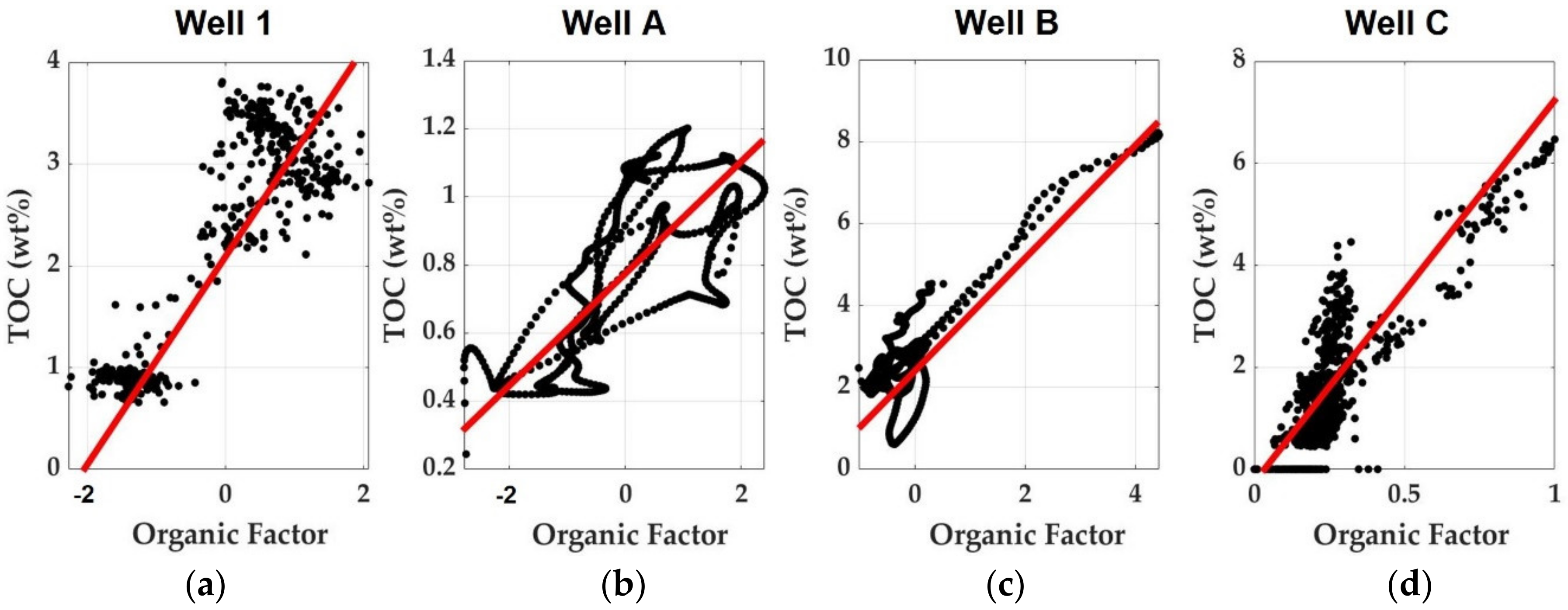
3.1. TOC Estimation Results

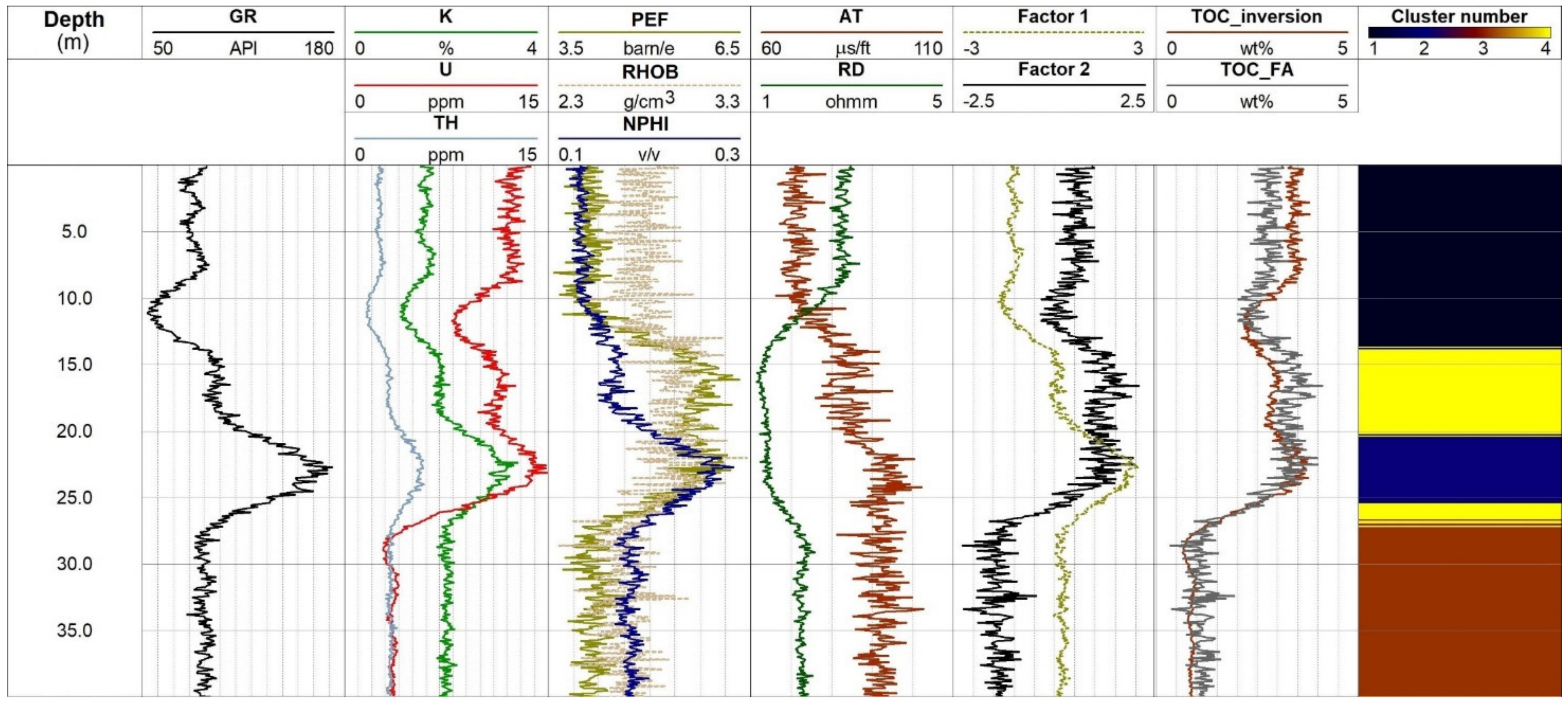
3.1.1. Synthetic Modeling Experiments

The wireline logs form a 401-by-9 theoretical log data matrix obtained from a model shale interval of 40 m in depth. Sampling rate of data is 0.1 m, and hence there are 401 data points. The well log suite includes the natural gamma-ray intensity (GR); spectral gamma-ray intensity logs such as uranium (U), thorium (TH) and potassium (K); photoelectric absorption index (PEF); density (gamma–gamma) (RHOB); sonic interval time of P-wave (AT); neutron porosity (NPHI); and deep (laterolog) resistivity (RD) logs. To mimic real well logging measurements, different amounts of random noise can be added to the above synthetic data computed by Equations (8)–(16). In this study, the kth noisy data at a given depth are computed as d k synthetic = d k 1 + Ν ( μ , σ ) , where the µ = 0 is the expected value and σ is the standard deviation proportional to the desired noise level. Based on this approach, we added 5% Gaussian distributed noise to the theoretical well logs calculated by Equations (8)–(16). Two statistical factors are extracted using Equation (4), and these new latent variables can be applied for quantitative description of the lithology (shale volume) and the organic content of the formation (TOC). The factor loadings estimated by Equation (3) are listed in Table 2. While the first factor (shale factor) had a high loading, especially for logs associated with the shale content of the formation (L(GR) = 0.91, L(K) = 0.97, L(TH) = 0.97), the uranium log which is more associated to the organic content of the logged interval had no correlation with it. However, a high loading was measured for the uranium log with the second factor (L(U) = 0.87, greater than other associated well logs), hence the term “organic factor”.
Regression analysis showed that the Pearson’s (linear) correlation coefficient between the organic factor and TOC (estimated from different sources such as inversion and core measurements) is high (R = 0.88). We minimize the cost function J(θ) (the error between the measured and estimated values of TOC) in iterative steps by using the gradient descent algorithm. The iteration steps preset for the regression analysis is 1000 steps with learning rates (𝛼) of 0.1, 0.3, 0.01, 0.03, 0.001 and 0.003. As a result, the regression coefficients entered into the empirical equation for TOC estimation, as defined in Equation (5), are 0.35, 3.75 and 3.24 for θ1, θ2 and J(θ), respectively. The regression model is illustrated in Figure 1a. In the same figure, we can compare the results of regression analyses of all wells involved in this study. As it is seen, the factor variable is unscaled, and it is inherently a standardized quantity. It is demonstrated that the suggested method gives consistent results and is applicable using different datasets and geological environments.
The results of factor analysis can be seen in Figure 2. In the first four tracks, the noisy synthetic wireline logs are plotted. The theoretical logs are calculated by Response Equations (8)–(16) and are contaminated with 5% Gaussian distributed noise. On the fifth track, the resultant factor logs can be seen. The first factor indicates the amount of shaliness, while the second one is proportional to the total organic content. On the sixth track, the organic content estimation results can be found. TOC_FA log is estimated from factor analysis, while TOC_inversion is the result of interval inversion using 20th-degree Legendre polynomials as basis functions in Equation (7). The independent results agree well and are also confirmed by the k-means cluster analysis of the same well logs [44]. The cluster number log calculated by nonhierarchical clustering using a robust weighted least squares distance metric as similarity criterion assumes four different lithology categories, where dark colors indicate the organic matter-rich (possible reservoir) intervals and lighter colors show shale deposits containing lower concentrations of uranium.

3.1.2. Results in Well A

Well logging data were previously collected in a Miocene tight gas interval in Derecske Trough, East Hungary. The input dataset includes the natural gamma-ray intensity log (GR); spectral gamma-ray intensity logs such as uranium (U), thorium (TH) and potassium (K); photoelectric absorption index log (PEF); bulk density log (RHOB); compensated neutron porosity log (NPHI); and shallow (RS) and deep (laterolog) resistivity (RD) logs. The loadings of the two extracted factors are included in Table 3. The natural gamma ray, thorium and potassium logs have an average loading (L) of 0.9, and the Uranium log has a factor loading of L(U) = 0.7. The organic factor shows a moderate correlation with total organic content in Well A (Figure 1b); this result is consistent with our synthetic modeling experiments. The Pearson’s correlation coefficient between the second factor and TOC is R = 0.74 (that between the first factor and inversion derived shale volume is R = 0.9). The regression coefficients (estimated in the same manner presented in Section 3.1.1) in Equation (5) are 0.38, 0.75 and 0.34 for θ1, θ2 and J(θ), respectively.
The results of factor analysis can be seen in Figure 3. The gamma-ray and porosity logs (bulk density (RHOB) and neutron porosity (NPHI)) show gas indications in the tight gas formation. In the first four tracks, the observed well logs are plotted. On the fifth track, the resultant factor logs can be seen; the first factor indicates the amount of shaliness, while the second one is proportional to the total organic content. On the sixth track, the organic content estimation results can be found. TOC_FA log as a result of factor analysis is validated by interval inversion (based on 40th-degree Legendre polynomials) estimation (TOC_inversion), artificial neural network prediction (TOC_ANN) and core laboratory measurements in some points (TOC_core). The agreement is acceptable, and the cluster analysis results highlight different intervals. The color codes of rock types are the same as in the synthetic case.

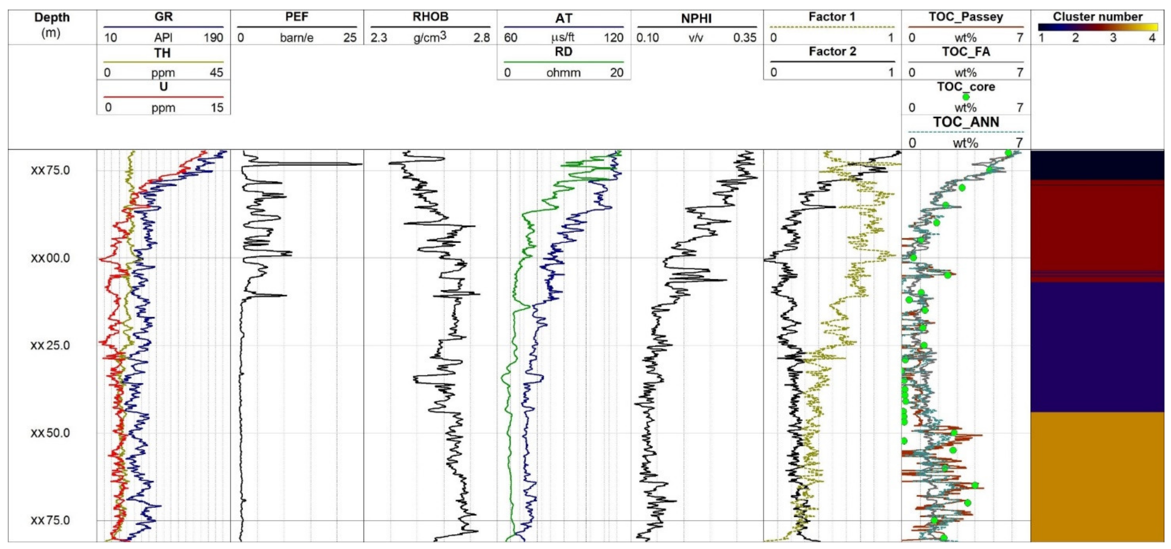
3.1.3. Results in Well B

The well interval processed is a shale gas reservoir in Alaska, USA. The available wireline logs are as follows: deep induction (RD), neutron porosity (NPHI), density (RHOB), sonic travel-time (AT) and natural gamma-ray (GR). The analyzed interval depth ranges from 3450 to 3500 m with 601 measured data points. The loadings of the two extracted factors are included in Table 4. The factor analysis result showed that, unlike in the previous two cases, the first factor had its highest correlation with the NPHI log, while that with the natural gamma-ray was low (0.12). Neuron porosity and bulk density logs are both highly sensitive to shale volume, which is also confirmed by the results of factor analysis. Despite this difference from the previous results, the first factor is still correlated highly with the shale volume (R = 0.84). On the other hand, the second factor, which correlates highly with the natural gamma-ray log (L(GR) = 0.96), has a very weak relation to shale volume (R = −0.22) and a strong correlation with TOC (R = 0.88) (Figure 1c). The regression parameters defined for the mathematical relationship between the organic factor and TOC are 1.79, 6.60 and 5.63 for θ1, θ2 and J(θ), respectively.
The results of factor analysis can be seen in Figure 4. The natural gamma-ray log shows high-intensity values around 3010 m; this zone is identified as a sweet spot. Cluster analysis separates four different zones; each contains some amount of kerogen most significantly in the black-colored zone (track 8). (The color codes of rock types are the same as in the previous cases.) In the first five tracks, the measured wireline logs are plotted. On the sixth track, the well logs of the two extracted factors can be seen. On the seventh track, the total organic content prediction results can be found: factor analysis (TOC_FA), interval inversion using 30th-degree Legendre polynomials (TOC_inversion), artificial neural network (TOC_ANN) and core analysis from literature resources (TOC_core). Different evaluation methods give consistent results; unfortunately, no core data can confirm the maximum of the TOC curve, which is given only by well log analysis.

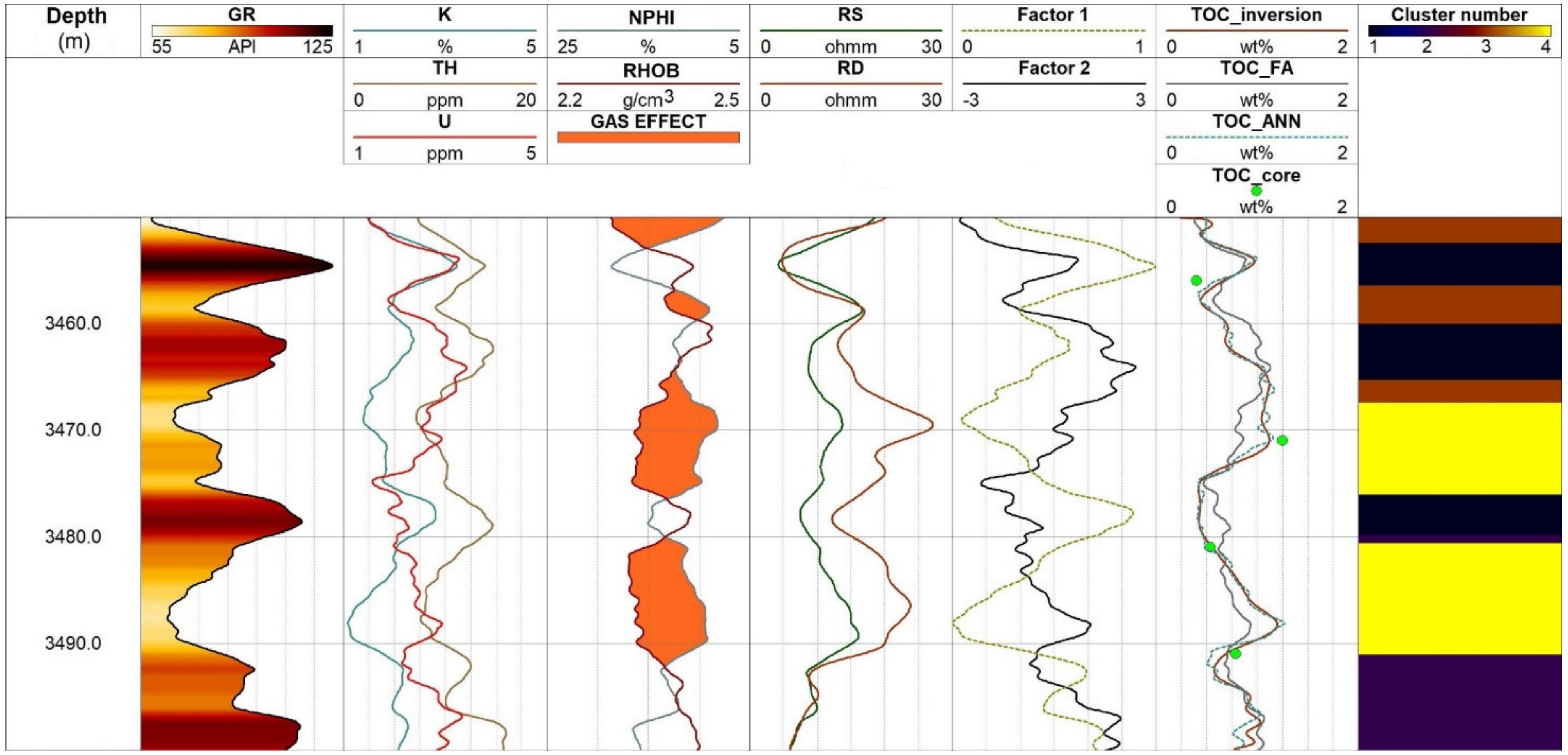
3.1.4. Results in Well C

The evaluation procedure is tested also in a Norwegian well. The processed wireline logs are as follows: natural gamma-ray intensity (GR), spectral gamma-ray intensity logs such as uranium (U) and thorium (TH) concentrations, photoelectric absorption index (PEF), bulk density (RHOB), acoustic travel-time (AT), neutron porosity (NPHI) and deep resistivity (RD). The factor loadings of the two statistical variables extracted from the above dataset are included in Table 5. From the point of view of TOC estimation, it is favorable that the uranium log has a high correlation with the organic factor (L(U) = 0.95), consistent with the previous wells where the uranium log is available. The second factor also has a relatively high measure of correlation with the sonic and resistivity logs, which also implies that the logs can be used to effectively estimate the TOC quantities for the section using Passey’s (ΔlogR) method.
The regression relationship between the organic factor and TOC is also valid in Well C. The regression analysis specified the parameters 0.14, 6.47 and 2.27 for θ1, θ2 and J(θ), respectively. The measured correlation coefficient between the two parameters is R = 0.84, and the straight line as a regression model can be seen in Figure 1d. The results of factor analysis can be studied in Figure 5. In the first five tracks, the observed well logs are plotted. In lithology logs, it can be seen that besides almost a constant rate of thorium concentration, the uranium content is mostly responsible for the total natural gamma-ray counts. The photoelectric absorption index log shows some mineral variations at the upper portion of the section, and an abundance of pyrite minerals causes the local maximal deflections of the PEF curve. On the sixth track, the well logs of the two extracted factors can be seen. Next to it, one can find the TOC estimations based on factor analysis (TOC_FA), the classical Passey’s method (TOC_Passey), artificial neural network (TOC_ANN) and core lab measurements (TOC_core). The clusters formed by the k-means clustering algorithm primarily indicate the TOC variation along the processed interval.

4. Discussion and Conclusions

Traditional Passey’s and modern inversion methods for TOC estimation have been applied along with the factor analysis approach described in this work. Core data have also been used to validate the results obtained. While the ΔlogR method relies only on the sonic and resistivity logs for the determination of TOC, the inversion-based methods process all suitable logs simultaneously, taking advantage of existing mathematical relationships (i.e., response equations) between the well logs and the organic content of the analyzed formations. Factor analysis, however, seeks latent factors within the same dataset that have some relationship with the parameter of interest for the estimation of that parameter, which in this case is the organic content.
It is observed that the regression parameters for the different wells vary, most probably due to the high variance associated with organic matter along vertical scales, even in a single formation. For comparing the results more easily, the factors can be properly scaled. In [4], this vertical heterogeneity was attributed directly to the geologic and biotic conditions under which these sediments were deposited. Selection of defined globally valid regression parameters for the estimation of TOC, therefore, most likely requires more statistical information/data analysis from surrounding wells and/or calibration of the extracted organic factor to TOC measured using lab-based geochemistry techniques, as noted in [15]. However, it is shown in our results that the factors extracted in various cases are unique to the formation and the wireline logs recorded for such formations.
Let us compare the factor loadings obtained from the studied wells (Table 6). In the first two wells, the natural gamma-ray, thorium, potassium, neutron porosity and resistivity logs have no significant correlation with the organic factor. The relationship between the relevant factor and organic content of the formation is, however, made evident in the synthetic case and in Wells 1, A and C (where uranium concentration data are available) with loadings of 0.87, 0.70 and 0.95, respectively. In Well B, it can be argued that the high factor loading between the second factor and natural gamma-ray may be a result of the high organic presence in the formation, as Table 4 shows that the well log has a very poor factor loading to the shale content of the formation.
The Passey’s overlay method was inapplicable in the first three cases due to the failure of the log calibration required by the procedure as described in [22]. The successful estimation of TOC by the suggested factor analysis technique therefore highlights an advantage of the method, as calibrations are not necessary for estimating organic contents of the formation. Because the extracted factor depends greatly on the original logs in the analyzed well, factors extracted from wells containing different datasets may lead to poor estimation of the parameters if the same regression coefficients are applied. Observations from the analyzed wells show that the vertical variability may be correct. The newly obtained TOC log requires calibration to data of core samples afterward.
In conclusion, it was demonstrated that the results of factor analysis are consistent and this approach gives reliable results for different well log suites and geological formations. This study was carried out using datasets from shale gas formations, tight gas sands sourced by adjacent lying source rocks and a source rock from a conventional reservoir. The inference drawn from the results obtained in this work showed that, of the two latent variables extracted, the first one is a shale indicator valid in organic matter-free intervals, while the second one is an organic factor indicating the presence of shale reservoirs. The empirical equation for estimating the parameters is site-specific and thus may not be applied globally. However, with the analysis of datasets from a similar field/formation, regression coefficients that work best for such areas can be determined. This work can be further developed to study the effects of level of maturity, kerogen type, depositional environments, etc., on the extracted organic factor and how this affects the absolute value of the TOC derived from factor analysis. The in situ estimation of the shale volume and TOC over a continuous interval can be extended to multidimensional applications using a 2D/3D factor analysis algorithm. All of the algorithms used in this study were developed in MATLAB and Python. To yield more robust estimation results, the current algorithm can be combined with other machine learning tools, such as hyperparameter estimation-based factor analyses. For instance, the control parameters of factor analysis can be automatically determined by hyperparameter estimation methods. As a result, TOC estimation can be made more effectively, reliably and accurately along a well or even between several wells.

Author Contributions

Conceptualization, N.P.S.; methodology, N.P.S., M.D.; software, A.U., S.T.; validation, R.V.-V., A.U., S.T.; formal analysis, A.U.; investigation, A.U., S.T.; resources, N.P.S., I.S.; data curation, R.V.-V., A.U., S.T.; writing—original draft preparation, N.P.S., R.V.-V., A.U., S.T.; writing—review and editing, N.P.S., M.D.; visualization, N.P.S., A.U.; supervision, I.S., M.D.; funding acquisition, N.P.S. All authors have read and agreed to the published version of the manuscript.

Funding

This research was funded by National Research, Development and Innovation Office, grant number K-135323.

Institutional Review Board Statement

Not applicable.

Informed Consent Statement

Not applicable.

Data Availability Statement

Not applicable.

Acknowledgments

The research was carried out in the Project No. K-135323 supported by the National Research, Development and Innovation Office (NKFIH), Hungary. The authors thank the Applied Research Institute of Earth Sciences, University of Miskolc, for providing the dataset of Well A. Thanks go to William Rouse and David Houseknecht from U.S. Geological Survey for providing the data of Well B and to MOL Plc. for providing the dataset of Well C.

Conflicts of Interest

The authors declare no conflict of interest.

References

  1. Zou, C. (Ed.) Unconventional Petroleum Geology, 2nd ed.; Elsevier: Amsterdam, Netherlands, 2017; Part 1, pp. 49–94. [Google Scholar]
  2. Bjørlykke, K. Unconventional hydrocarbons: Oil shales, heavy oil, tar sands, shale gas and gas hydrates. In Petroleum Geosciences; Springer: Berlin/Heidelberg, Germany, 2010; pp. 459–465. [Google Scholar] [CrossRef]
  3. Sun, S.Z.; Sun, Y.; Sun, C.; Liu, Z.; Dong, N. Methods of calculating total organic carbon from well logs and its application on rock’s properties analysis. Geoconvention Integr. 2013, 1–7. [Google Scholar]
  4. Passey, Q.; Kevin, B.; William, E.; Robert, K.; Somnath, S. From oil-prone source rock to gas-producing shale reservoir—Geologic and petrophysical characterization of unconventional shale gas reservoirs. Soc. Pet. Eng. 2010, 31350. [Google Scholar] [CrossRef]
  5. Valadez Vergara, R. Well-log based TOC estimation using linear approximation methods. Geosci. Eng. 2020, 8, 116–130. [Google Scholar]
  6. Lawley, D.N.; Maxwell, A.E. Factor analysis as a statistical method. J. R. Stat. Soc. Ser. D 1962, 12, 209–229. [Google Scholar] [CrossRef]
  7. Király, A.; Milota, K.; Magyar, I.; Kiss, K. Tight gas exploration in the Pannonian Basin. In Geological Society, London, Petroleum Geology Conference Series; Geological Society of London: London, UK, 2010; Volume 7, pp. 1125–1129. [Google Scholar] [CrossRef]
  8. Haás, J. (Ed.) Geology of Hungary; Springer: Berlin/Heidelberg, Germany, 2013. [Google Scholar]
  9. Houseknecht, D.W.; Bird, K.J. Sequence stratigraphy of the Kingak shale (Jurassic–Lower cretaceous), national petroleum reserve in Alaska. AAPG Bull. 2004, 88, 279–302. [Google Scholar] [CrossRef]
  10. Rouse, W.A.; Houseknecht, D.W. Modified method for estimating petroleum source-rock potential using wireline logs, with application to the Kingak Shale, Alaska North Slope, vols. 2016–5001. In U.S. Geological Survey Scientific Investigations Report; USGS Publications Warehouse: Reston, VA, USA, 2016; p. 40. [Google Scholar]
  11. Detterman, R.L.; Reiser, H.N.; Brosge, W.P.; Dutro, J.T., Jr. Post-Carboniferous Stratigraphy, Northeastern Alaska; US Geological Survey Professional Paper 886; USGS Publications Warehouse: Reston, VA, USA, 1975; 46p.
  12. Reiser, H.N.; Brosge, W.P.; Dutro, J.T., Jr.; Detterman, R.L. Geologic map of the demarcation point quadrangle, Alaska. In U.S. Geological Survey Miscellaneous Investigations Series Map; 1 Sheet, Scale 1:250,000; USGS Publications Warehouse: Reston, VA, USA, 1980; p. 1133. [Google Scholar]
  13. Magoon, L.B.; Claypool, G.E. The Kingak shale of northern Alaska—Regional variations in organic geochemical properties and petroleum source rock quality. Org. Geochem. 1984, 6, 533–542. [Google Scholar] [CrossRef]
  14. Vollset, J.; Doré, A.G. A revised triassic and jurassic lithostratigraphic nomenclature for the Norwegian North Sea. In NPD-Bulletin; Norwegian Petroleum Directorate: Stavanger, Norway, 1984. [Google Scholar]
  15. Peters, K.E.; Xia, X.; Pomerantz, A.E.; Mullins, O.C. Geochemistry applied to evaluation of unconventional resources. In Unconventional Oil and Gas Resources Handbook; Zee, M.Y., Holditch, S.A., Eds.; Gulf Professional Publishing: Houston, TX, USA, 2016; pp. 71–126. [Google Scholar] [CrossRef]
  16. Beers, R.F.; Goodman, C. Distribution of radioactivity in ancient sediments. GSA Bull. 1944, 55, 1229–1254. [Google Scholar] [CrossRef]
  17. Fertl, W.H.; Chilingar, G.V. Total organic carbon content determined from well logs. SPE Form. Eval. 1988, 3, 407–419. [Google Scholar] [CrossRef]
  18. Fertl, W.H.; Rieke, H.H.I. Gamma ray spectral evaluation techniques identify fractured shale reservoirs and source-rock characteristics. J. Pet. Technol. 1980, 32, 2053–2062. [Google Scholar] [CrossRef]
  19. Schmoker, J.W. Determination of organic content of Appalachian Devonian Shales from formation-density logs: Geologic notes. AAPG Bull. 1979, 63, 1504–1509. [Google Scholar] [CrossRef]
  20. Schmoker, J.W.; Hester, T.C. Organic carbon in Bakken Formation, United States Portion of Williston Basin. AAPG Bull. 1983, 67, 2165–2174. [Google Scholar] [CrossRef]
  21. Zhao, P.; Mao, Z.; Huang, Z.; Zhang, C.A. New method for estimating total organic carbon content from well logs. AAPG Bull. 2016, 100, 1311–1327. [Google Scholar] [CrossRef]
  22. Passey, Q.R.; Creaney, S.; Kulla, J.B.; Moretti, F.J.; Stroud, J.D. A practical model for organic richness from porosity and resistivity logs. AAPG Bull. 1990, 74, 1774–1794. [Google Scholar]
  23. Glorioso, J.C.; Rattia, A.J. Unconventional reservoirs: Basic petrophysical concepts for shale gas. In SPE/EAGE European Unconventional Resources Conference & Exhibition-from Potential to Production; European Association of Geoscientists & Engineers: Houten, The Netherlands, 2012. [Google Scholar] [CrossRef]
  24. Bibor, I.; Szabó, N.P. Unconventional shale characterization using improved well logging methods. Geosci. Eng. 2016, 5, 32–50. [Google Scholar]
  25. Jöreskog, K.G. Factor analysis and its extensions. In Factor Analysis at 100, Historical Developments and Future Directions; Cudeck, R., MacCallum, R.C., Eds.; Lawrence Erlbaum Associates: Mahwah, NJ, USA, 2007; pp. 47–77. [Google Scholar]
  26. Szabó, N.P.; Dobróka, M. Extending the application of a shale volume estimation formula derived from factor analysis of wireline logging data. Math. Geosci. 2013, 45, 837–850. [Google Scholar] [CrossRef]
  27. Odokuma-Alonge, O.; Adekoya, J.A. Factor analysis of stream sediment geochemical data from Onyami Drainage System, Southwestern Nigeria. Int. J. Geosci. 2013, 4, 656–661. [Google Scholar] [CrossRef] [Green Version]
  28. Kaiser, H.F. The varimax criterion for analytical rotation in factor analysis. Psychometrika 1958, 23, 187–200. [Google Scholar] [CrossRef]
  29. Bartlett, M.S. The statistical conception of mental factors. Br. J. Psychol. 1937, 28, 97–104. [Google Scholar] [CrossRef]
  30. Szabó, N.P.; Dobróka, M. Exploratory factor analysis of wireline logs using a Float-Encoded Genetic Algorithm. Math. Geosci. 2018, 50, 317–335. [Google Scholar] [CrossRef]
  31. Szabó, N.P.; Dobróka, M. Robust estimation of reservoir shaliness by iteratively reweighted factor analysis. Geophysics 2017, 82, D69–D83. [Google Scholar] [CrossRef] [Green Version]
  32. Szabó, N.P. Shale volume estimation based on the factor analysis of well-logging data. Acta Geophys. 2011, 59, 935–953. [Google Scholar] [CrossRef]
  33. Mayer, C.; Sibbit, A. GLOBAL, a new approach to computer-processed log interpretation, paper SPE-9341. In Proceedings of the 55th SPE Annual Fall Technical Conference and Exhibition, Dallas, TX, USA, 21–24 September 1980; pp. 1–14. [Google Scholar]
  34. Dobróka, M.; Szabó, N.P. The inversion of well log data using Simulated Annealing method. Publs. Univ. Miskolc Geosci. A Min. 2001, 59, 115–137. [Google Scholar]
  35. Dobróka, M.; Szabó, N.P.; Tóth, J.; Vass, P. Interval inversion approach for an improved interpretation of well logs. Geophysics 2016, 81, D155–D167. [Google Scholar] [CrossRef] [Green Version]
  36. Szabó, N.P.; Dobróka, M. Series expansion-based genetic inversion of wireline logging data. Math. Geosci. 2019, 51, 811–835. [Google Scholar] [CrossRef]
  37. Szabó, N.P.; Dobróka, M. Interval inversion as innovative well log interpretation tool for evaluating organic-rich shale formations. J. Petrol. Sci. Eng. 2020, 186, 106696. [Google Scholar] [CrossRef]
  38. Mahmoud, A.A.A.; Elkatatny, S.; Mahmoud, M.; Abouelresh, M.; Abdulraheem, A.; Ali, A. Determination of the total organic carbon (TOC) based on conventional well logs using Artificial Neural Network. Int. J. Coal Geol. 2017, 179, 72–80. [Google Scholar] [CrossRef]
  39. McCulloch, W.S.; Pitts, W. A logical calculus of the ideas immanent in nervous activity. Bull. Math. Biol. 1990, 52, 99–115; discussion 73–97. [Google Scholar] [CrossRef]
  40. Morris, R.G.; Hebb, D.O. The organization of behavior. Brain Res. Bull. 1999, 50, 437. [Google Scholar] [CrossRef]
  41. Rumelhart, D.E.; Hinton, G.E.; Williams, R.J. Learning representations by back-propagating errors. Nature 1986, 323, 533–536. [Google Scholar] [CrossRef]
  42. Zych, M.; Stachura, G.; Hanus, R.; Szabó, N.P. Application of artificial neural networks in identification of geological formations on the basis of well logging data—A comparison of computational environments’ efficiency. In Methods and Techniques of Signal Processing in Physical Measurements, Lecture Notes in Electrical Engineering; Springer International Publishing: Cham, Switzerland, 2019; pp. 416–422. [Google Scholar] [CrossRef]
  43. Kingma, D.P.; Jimmy, B. Adam: A method for stochastic optimization. In Proceedings of the International Conference on Learning Representations, San Diego, CA, USA, 7 May 2015; Available online: https://arxiv.org/pdf/1412.6980.pdf (accessed on 15 September 2021).
  44. Szabó, N.P.; Nehéz, K.; Hornyák, O.; Piller, I.; Deák, C.; Hanzelik, P.P.; Kutasi, C.; Ott, K. Cluster analysis of core measurements using heterogeneous data sources: An application to complex Miocene reservoirs. J. Pet. Sci. Eng. 2019, 178, 575–585. [Google Scholar] [CrossRef]
Figure 1. TOC vs. organic (second) factor regression plots: (a) synthetic modeling case (R = 0.87); (b) Pannonian Basin, Hungary (Well A) (R = 0.74); (c) Alaska, USA (Well B) (R = 0.88); (d) North Sea, Norway (Well C) (R = 0.84).
Energies 14 05978 g001
Figure 2. Result of factor analysis in Well 1. Denotations are as follows: natural gamma-ray (GR), spectral gamma-ray (K, U, TH), photoelectric absorption index (PEF), bulk density (RHOB), neutron porosity (NPHI), acoustic travel-time (AT), deep resistivity (RD), TOC log from interval inversion (TOC_inversion) and TOC log from factor analysis (TOC_FA). The shale factor is Factor 1; the organic factor is Factor 2. The last track shows the depth distribution of four identified clusters.
Energies 14 05978 g002
Figure 3. Result of factor analysis in Well A. Denotations are as follows: natural gamma-ray (GR), spectral gamma-ray (K, TH, U), neutron porosity (NPHI), bulk density (RHOB), shallow (RS) and deep resistivity (RD), TOC estimates from interval inversion (TOC_inversion), TOC estimates from factor analysis (TOC_FA) and TOC estimates of artificial neural network (TOC_ANN). The shale factor is Factor 1; the organic factor is Factor 2. The last track shows the depth distribution of four identified clusters.
Energies 14 05978 g003
Figure 4. Result of factor analysis in Well B. Denotations are as follows: natural gamma-ray (GR), bulk density (RHOB), neutron porosity (NPHI), sonic travel-time (AT), deep induction resistivity (RD), first factor (Factor 1), second factor (Factor 2), TOC estimates from interval inversion (TOC_inversion), TOC estimates from the factor analysis (TOC_FA) and TOC estimates of artificial neural network (TOC_ANN). The last track shows the depth distribution of four identified clusters.
Energies 14 05978 g004
Figure 5. Result of factor analysis in Well C. Denotations are are follows: natural gamma-ray (GR), thorium concentration (TH), uranium concentration (U), photoelectric absorption factor (PEF), bulk density (RHOB), acoustic travel-time (AT), deep resistivity (RD), neutron porosity (NPHI), first factor (Factor 1), second factor (Factor 2), TOC estimates from Passey’s method (TOC_Passey), TOC estimates from the factor analysis (TOC_FA), TOC estimates of artificial neural network (TOC_ANN) and TOC estimates measured on core samples (TOC_core). The last track shows the depth distribution of four identified clusters.
Energies 14 05978 g005
Table 1. Well logging data summary of the analyzed wells.
LocationIndexInterval LengthWell Log Suite
Fictitious placeWell 140 mGR, K, U, TH, PEF, RHOB, NPHI, AT, RD
HungaryWell A50 mGR, K, TH, U, NPHI, RHOB, RD, RS
USAWell B92 mGR, AT, RHOB, NPHI, RD
NorwayWell C110 mAT, GR, NPHI, PEF, RD, RHOB, TH, U
Table 2. Factor loadings rotated using the varimax algorithm for Well 1.
Well LogShale Factor (F1)Organic Factor (F2)
GR0.910.32
K0.970.09
U−0.030.87
TH0.970.12
PEF0.560.64
RHOB0.200.60
AT0.76−0.43
NPHI0.95−0.01
RD−0.65−0.22
Table 3. Factor loadings rotated using the varimax algorithm for Well A.
Well LogShale Factor (F1)Organic Factor (F2)
GR0.930.36
K0.98−0.06
TH0.810.50
U0.080.70
NPHI0.890.25
RHOB0.650.49
RS−0.81−0.35
RD−0.79−0.17
Table 4. Factor loadings rotated using the varimax algorithm for Well B.
Well LogShale Factor (F1)Organic Factor (F2)
RD−0.900.05
NPHI0.910.37
GR0.120.96
RHOB−0.73−0.49
AT0.840.39
Table 5. Factor loadings rotated using the varimax algorithm for Well C.
Well LogShale Factor (F1)Organic Factor (F2)
AT0.700.68
GR0.240.89
NPHI0.700.66
PEF0.530.17
RD0.450.86
RHOB−0.40−0.58
TH0.830.15
U0.160.95
Table 6. Comparison of the loadings of the organic (second) factor for the analyzed unconventional hydrocarbon wells. Symbol (-) indicates no available logs.
Wireline LogFactor Loading (L(F2))
Well 1Well AWell BWell C
GR0.320.360.960.89
K0.09−0.06--
U0.870.7-0.95
TH0.120.5-0.15
PEF0.64--0.17
RHOB0.600.49−0.49−0.58
AT−0.43-0.390.68
NPHI−0.010.250.370.66
RD−0.22−0.170.050.86
RS-−0.35--
Publisher’s Note: MDPI stays neutral with regard to jurisdictional claims in published maps and institutional affiliations.

