Article

Hydrodynamic Analysis of Twin-Hull Structures Supporting Floating PV Systems in Offshore and Coastal Regions

by
Alexandros Magkouris
1,
Kostas Belibassakis
1 and
Eugen Rusu
2,*
1
School of Naval Architecture & Marine Engineering, National Technical University of Athens, 15780 Athens, Greece
2
Department of Mechanical Engineering, University Dunarea de Jos of Galati, 800008 Galati, Romania
*
Author to whom correspondence should be addressed.
Energies 2021, 14(18), 5979; https://doi.org/10.3390/en14185979
Submission received: 19 August 2021 / Revised: 11 September 2021 / Accepted: 16 September 2021 / Published: 20 September 2021
(This article belongs to the Topic Marine Renewable Energy)

Abstract

:
In this paper, a novel model based on the boundary element method (BEM) is presented for the hydrodynamic analysis of floating twin-hull structures carrying photovoltaic panels, supporting the study of wave responses and their effects on power performance in variable bathymetry regions. The analysis is restricted to two spatial dimensions for simplicity. The method is free of any mild-slope assumptions. A boundary integral representation is applied for the near field in the vicinity of the floating body, which involved simple (Rankine) sources, while the far field is modeled using complete (normal-mode) series expansions that are derived using separation of variables in the constant depth half-strips on either side of the middle, non-uniform domain, where the depth exhibited a general variation, overcoming a mild bottom-slope assumption. The numerical solution is obtained by means of a low-order panel method. Numerical results are presented concerning twin-hull floating bodies of simple geometry lying over uniform and sloping seabeds. With the aid of systematic comparisons, the effects of the bottom slope and curvature on the hydrodynamic characteristics (hydrodynamic coefficients and responses) of the floating bodies are illustrated and discussed. Finally, the effects of waves on the floating PV performance are presented, indicating significant variations of the performance index ranging from 0 to 15% depending on the sea state.

1. Introduction

The energy yield of floating photovoltaics (FPVs) is in the spotlight, as offshore photovoltaic (PV) installations present significant advantages over corresponding onshore ones (see [1,2]). These, among others, include the ample surface available for arrangements in farms, the nearshore/coastal regions and the open sea, including locations that are already licensed for offshore wind parks (in the area between wind turbines), as well as the potential of hybridization with offshore wind energy. The development of offshore FPV parks is particularly important for southern European regions, e.g., in the Mediterranean Sea, since solar radiation in southern latitudes is relatively high, nearly 150–200% greater than that of the Atlantic Sea Ocean, the North Sea and Baltic Sea regions [3], while wind and wave potentials are comparatively low. Furthermore, offshore PV installations present increased efficiency due to the cooling effects of water and wind, which are triggered by the interaction of airflow with the solar panels [4]. It is worth mentioning here that, according to a recent report from DNV GL, it is expected that offshore FPVs will reach maturity by 2030 (see also DNVGL-RP-0584-Edition 2021-03).
On the other hand, although several solar farms have been developed on closed water basins, such as lakes, reservoirs and dams, implementing installations in the open sea is a challenging task, as their interaction with several environmental factors is not yet fully understood [5]. In the offshore and nearshore region, safety and viability require the design and construction of resilient FPV structures that can withstand the harsh marine environment. Regarding the deployment of floating structures of relatively large dimensions in nearshore and coastal areas, it is also expected that bathymetric variations will have significant effects on their responses under wave loads, which also affect the performance of the power output due to oscillatory motions of the structure and the panels arranged on the deck. Stability requirements, in conjunction with a lightweight structure with a center of gravity at a relatively increased height above the keel, led to the consideration of a twin hull structure with a more complicated response pattern and resonance characteristics. In this study, a hydrodynamic model is developed to predict the dynamic responses of a floating structure supporting photovoltaic panels on a deck while being subject to wave loads. For the treatment of complicated resonance phenomena, as well as the effects of finite and possibly variable bathymetry, which characterizes nearshore and coastal regions, a general model based on boundary element methods (BEM) is developed, which is capable of modeling the involved phenomena. The model is then systematically applied in selected examples to produce preliminary results, which are illustrative of the effect of dynamic motions on the energy efficiency of a floating unit.
The interaction of free surface gravity waves with floating bodies at intermediate depths in areas that are characterized by non-uniform seabed topographies is a mathematically interesting problem, which can be used to analyze a wide range of applications, such as the design and performance evaluation of ships and other floating structures operating in nearshore areas. Theoretical aspects of the problem of small-amplitude water waves propagating in a finite water depth and their interaction with floating and/or submerged bodies have been presented under various geometric assumptions by many authors [6,7,8] regarding the existence of trapped modes in a channel with obstructions. Furthermore, shallow-water conditions are frequently encountered in marine applications. When floating structures or docks are moored in shallow-water areas, accurate predictions of the motions induced by the prevailing sea state are needed, not only for optimizing the mooring system, depending on the stability needs of each configuration, but also for ensuring that the under-keel clearance remains sufficient for the structure to avoid grounding in extreme (for the area under study) weather and sea conditions. In many applications, the water depth is assumed to be constant, which is practically valid in cases where there are small depth variations or the floating body’s dimensions are small compared to the bottom variation length. However, in applications involving the utilization of floating bodies in coastal waters, the variations of bathymetry may cause significant effects on the hydrodynamic behavior of ships and structures, especially concerning the wave-induced responses. Under the assumption of slowly varying bathymetry, mild-slope model have been developed for the analysis of wave-induced floating body motion [9]. To treat environments that are characterized by steeper bathymetric variations, e.g., near the coast or the entrances of ports and harbors, extended models are required (see, e.g., Ohyama and Tsuchida [10]).
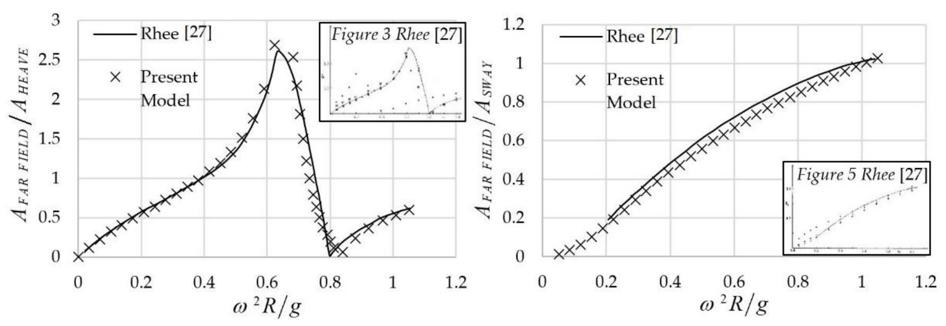
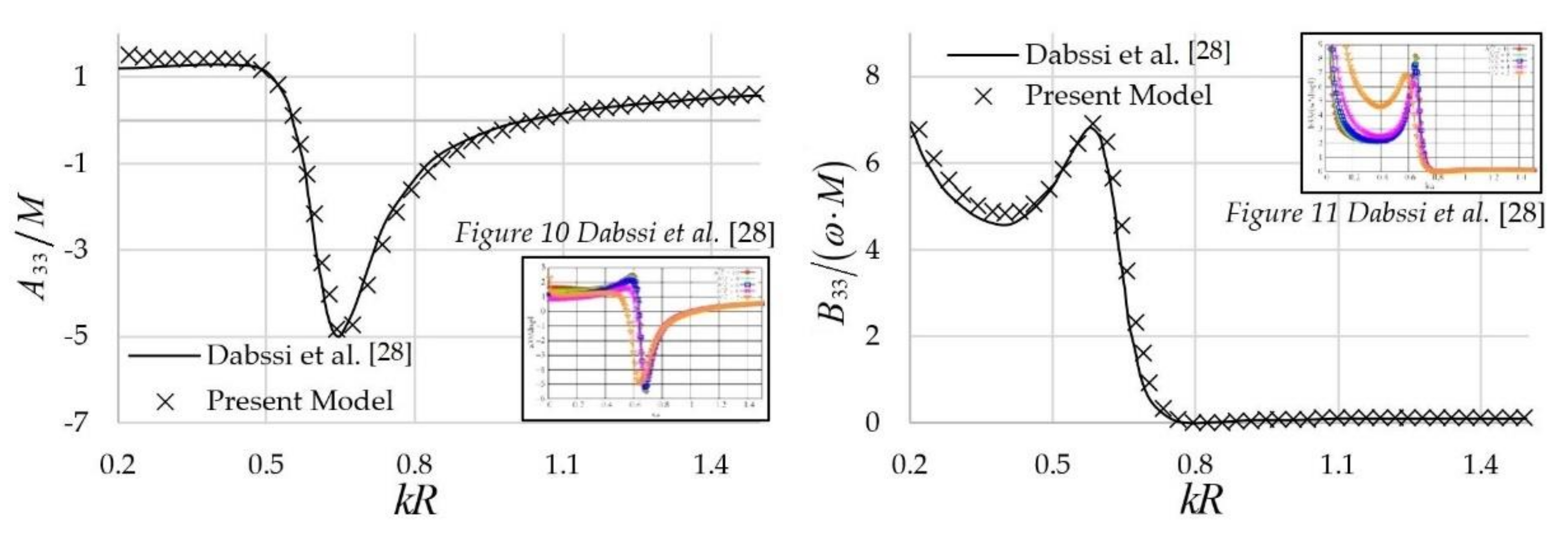
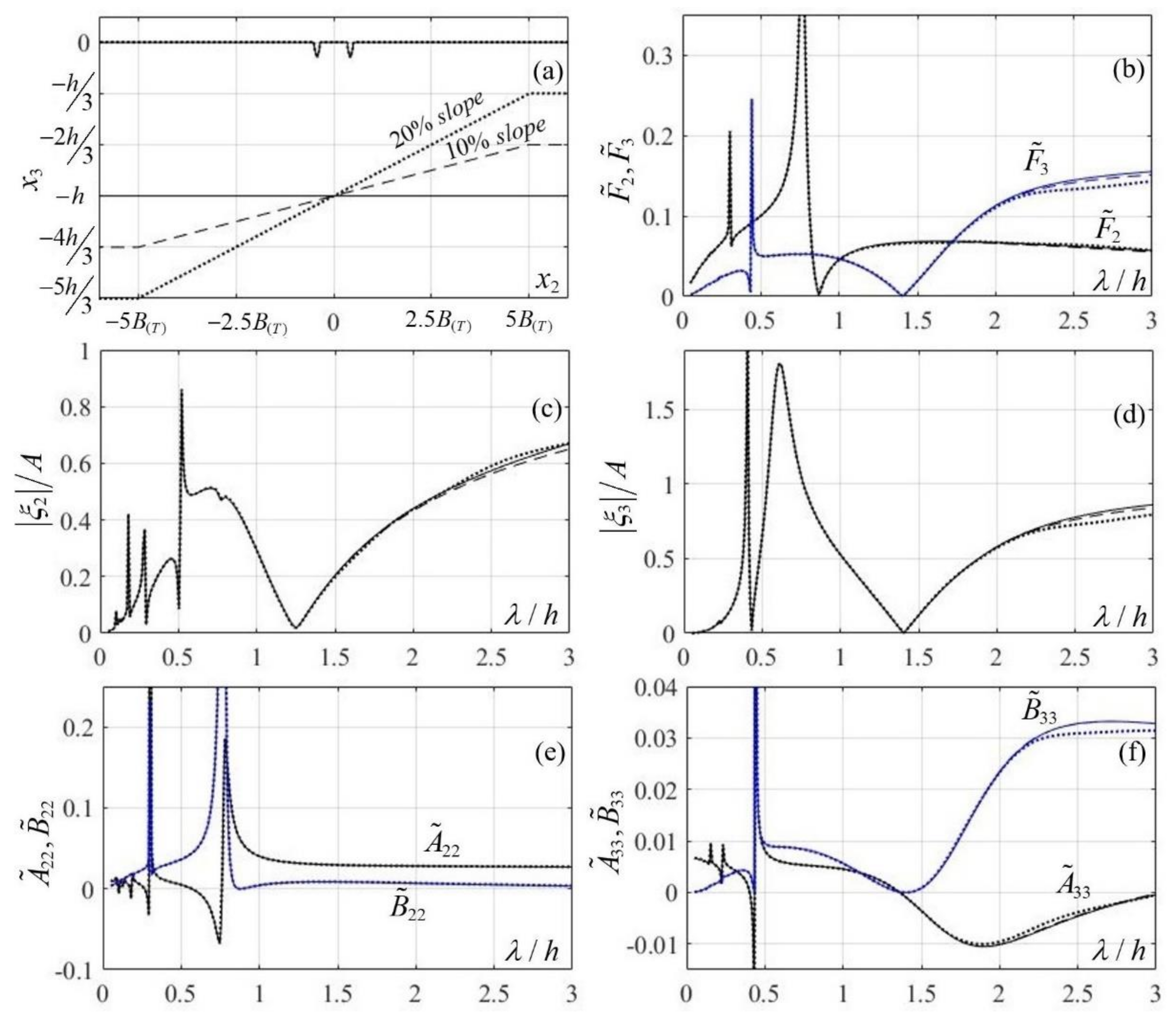
In the present work, a novel method based on BEM is used for the hydrodynamic analysis of twin-hull floating structures with PV systems; the method is capable of treating the effects of varying bathymetry without any mild-slope assumptions. In particular, a low-order panel based on linear wave theory is developed and verified. Following the hybrid formulation by Yeung [11], the present method utilizes the simplicity of Rankine sources, in conjunction with appropriate representations of the wavefield in the exterior semi-infinite domain, as presented by Nestegard and Sclavounos [12] for 2D radiation problems in deep water and by Drimer and Agnon [
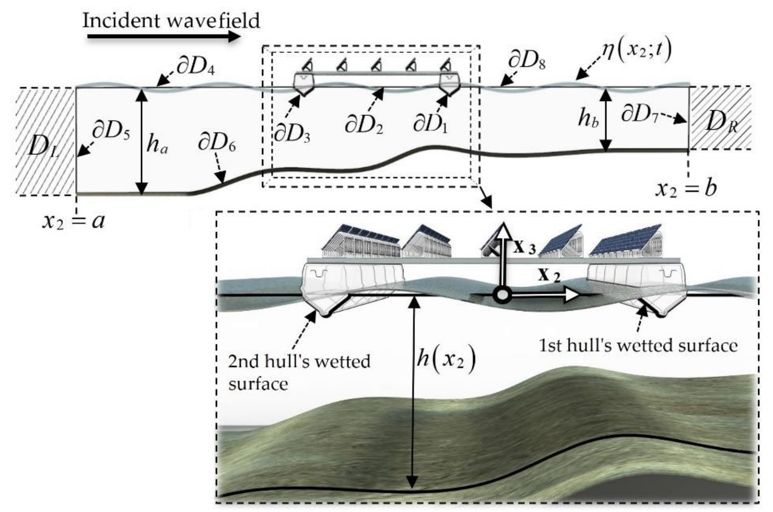
13] in the case of finite water depth. Τhe far field is modeled using complete (normal-mode) series expansions, which are derived using separation of variables in the two constant-depth half-strips separating the variable bathymetry region from the regions of wave incidence and wave transmission (see Figure 1). Numerical results are presented concerning twin-hull floating bodies of simple geometry over uniform and sloping seabeds. With the aid of systematic comparisons, the effects of bottom slope on the hydrodynamic characteristics (hydrodynamic coefficients and responses) are presented and discussed. Finally, results are presented regarding the effect of wave-induced motions on floating PV performance, indicating significant variations in the performance index ranging from 0 to 15%, depending on the sea state.

2. Mathematical Formulation

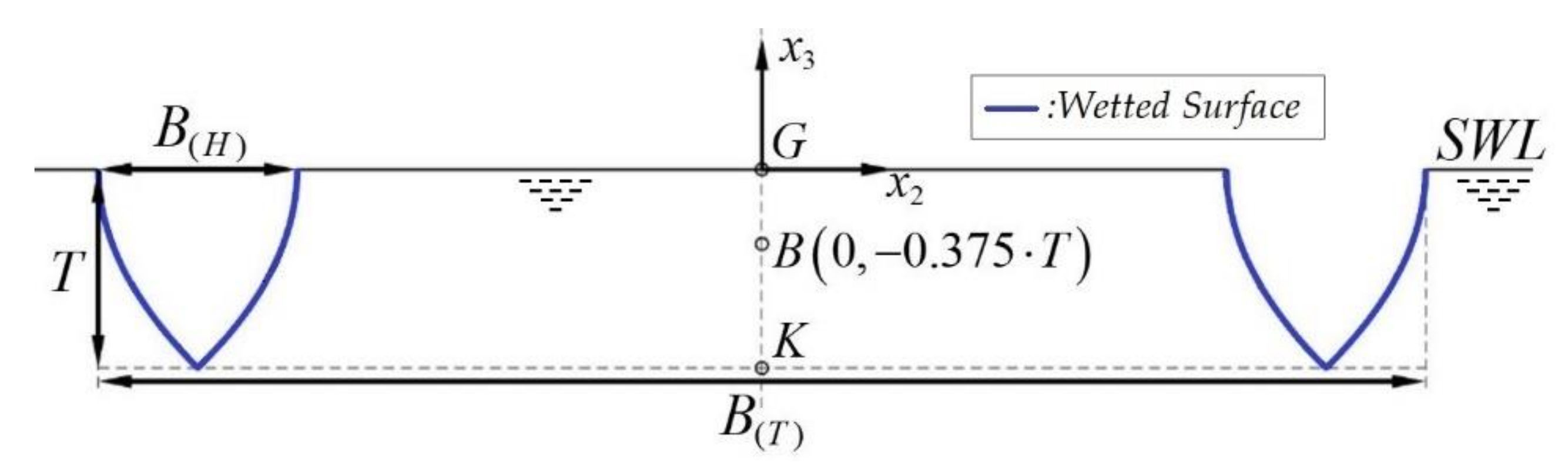
The 2D problem concerning the hydrodynamic behavior of a twin hull floating body of arbitrary cross-section in a coastal–marine environment is considered, as illustrated in Figure 1. A Cartesian coordinate system x = ( x 1 , x 2 , x 3 ) is introduced, with the origin placed at the mean water level, coinciding with the structure’s center of flotation, with the x 3 -axis pointing upwards. The configuration is considered unchanged in the x 1 -direction and, therefore, the analysis is limited to the x 2 x 3 plane, modeling a two-dimensional cross-section.
The environment comprises a water layer bounded by the free surface at x 3 = 0 and the rigid bottom at depth h = h ( x 2 ) . It is assumed that h = h ( x 2 ) exhibited a general variation, i.e., the corresponding bathymetry is defined by parallel, straight contours lying between two regions of constant but different water depths: h = h a in the region of wave incidence and h = h b in the region of transmission. The fluid is assumed to be homogeneous, inviscid and incompressible and its motion irrotational with a small width. The wavefield in the region is excited by a harmonic incident field, with propagation direction normal to the depth contours (along the x 2 -axis). Without loss of generality, a left-incident wave field is assumed (see Figure 1). Thus, in the context of linearized wave theory, the fluid motion is fully described by the 2D wave potential Φ x 2 , x 3 ; t , with the velocity field being equal to v x , t = Φ x , t . Assuming that the free-surface elevation and the wave velocities are small, the potential function Φ x 2 , x 3 ; t satisfies the linearized wave equations (see, e.g., [14,15]). Under these assumptions, the wavefield is time-harmonic and its potential function can be represented by the time-independent (normalized) complex potential function φ as:
Φ x 2 , x 3 ; t = Re i g A ω φ x 2 , x 3 ; μ exp i ω t ,
where H = 2 A is the incident wave height, g is the acceleration of gravity, μ = ω 2 / g is the frequency parameter and i = 1 . The free surface elevation is obtained in terms of the wave potential at x 3 = 0 as follows:
η x 2 ; t = 1 g Φ x 2 , 0 ; t t .
In addition to the physical boundaries (floating body, free surface, seabed), we further introduce two vertical interfaces on either side of the body, serving as incidence/radiation/transmission boundaries. Therefore, the boundary D of the two-dimensional domain D , occupied by the fluid, is decomposed into eight subsections D i ,   i = 1 , 2 , , 8 , as illustrated in Figure 1, so that D is enclosed by the curve D = i = 1 8 D i , with D 1 and D 3 being the right- and left-hand sides, respectively, of the twin-hull’s wetted surface. The sections of D numbered 2, 4 and 8 correspond to the water-free surface, while D 6 is the impermeable seabed. Finally, the wave incidence occurs via D 5 , which also serves, along with D 7 , as a radiation interface for the diffracted field due to the presence of the (fixed) body, as well as the radiation fields that develop due to the wave-induced body’s motions.
Apart from the non-uniform domain D containing the floating body, the total flow field is considered to be of infinite length and, therefore, also comprises the uniform semi-infinite subdomains D L and D R , where the depth is constant and equal to h a and h b , respectively. Hence, the function h = h ( x 2 ) is of the form:
h x 2 = h a , x 2 a h x 2 ,   a < x 2 < b h b , x 2 b
The function φ = φ x 2 , x 3 ; μ appearing in Equation (1) is the normalized potential in the frequency domain, which will hereafter be simply written as φ x 2 , x 3 . Using standard floating body hydrodynamic theory [15,16], the potential is decomposed as follows:
φ x 2 , x 3 = φ p x 2 , x 3 + μ A k = 2 4 ξ k φ k x 2 , x 3
where φ p x 2 , x 3 = φ I x 2 , x 3 + φ D x 2 , x 3 is the propagating field, with φ I x 2 , x 3 being the incident field, which corresponds to the solution of the wave propagation problem across the non-uniform subdomain in the absence of the floating structure and φ D x 2 , x 3 
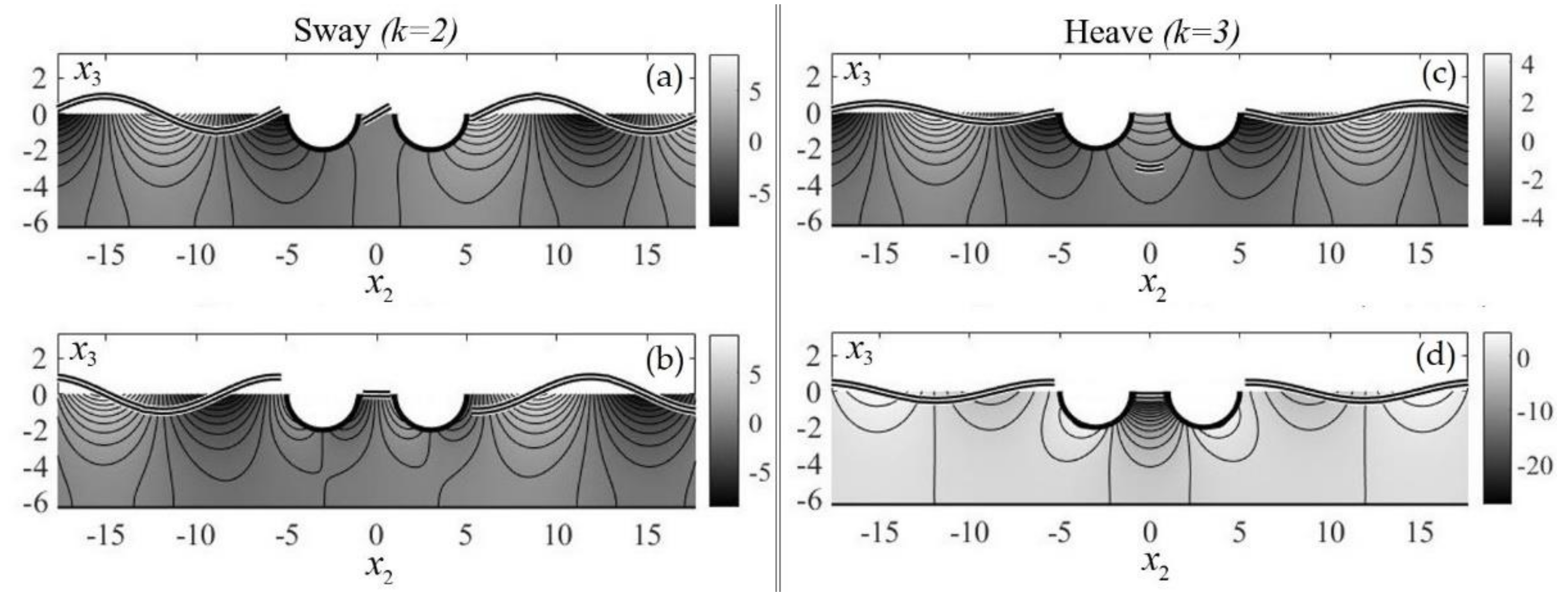
being the diffraction potential, which accounts for the presence of the body, fixed in its mean position. Moreover, the functions φ k x 2 , x 3 ,   k = 2 , 3 , 4 , denote the radiation potentials associated with the motion of the twin-hull structure, corresponding to its three degrees of freedom (DOF), i.e., the linear transverse motion (sway: k = 2), the linear vertical motion (heave: k = 3) and the rotation about the longitudinal ( x 1 ) axis (roll: k = 4). Finally, ξ k ,   k = 2 , 3 , 4 , stand for the complex amplitudes of the corresponding wave-induced motions.
The sub-problems, whose solutions provide the potential functions φ k x 2 , x 3 ,   k = p , 2 , 3 , 4 , in the variable bathymetry region, were formulated as radiation-type problems in the bounded subdomain D , with the aid of the following general representations of the wave potential φ x 2 , x 3 in the left- and right-side semi-infinite strips D L and D R , which are obtained using separation of variables (see, e.g., [17]):
φ p ( L ) x = exp i k 0 L x 2 + C 0 L exp i k 0 L x 2 Z 0 L x 3 +     + n = 1 C n L exp k n L x 2 a Z n L x 3 , x D L
φ k ( L ) x = C 0 L exp i k 0 L x 2 Z 0 L x 3 +     + n = 1 C n L exp k n L x 2 a Z n L x 3 , x D L , k = 2 , 3 , 4
φ k ( R ) x = C 0 R exp i k 0 R x 2 Z 0 R x 3     + n = 1 C n R Z n R x 3 exp k n R b x 2 ,   x D R ,   k = p , 2 , 3 , 4
The first term n = 0 in the series Equations (5) is the propagating mode, while the remaining ones n = 1 , 2 , are the evanescent modes with C n ( i ) n = 0 , 1 , 2 , being the corresponding coefficients. The first term of φ p ( L ) x is further separated into a unit-amplitude mode propagating toward D, playing the role of the incident field, and the additional mode C 0 L exp ( i k 0 L x 2 ) Z 0 L ( x 3 ) , propagating toward in the x 2 -direction, which is the reflected field coming from the diffraction potential φ D x . In the above expansions, the functions { Z n ( i ) } n = 0 are defined as Z n i = cosh k n ( i ) z + h ( i )   /   cosh k n ( i ) h ( i ) and are obtained using separation of variables via the vertical Sturm–Liouville problem, to which Laplace’s equation reduces in the constant depth strips D L h a < x 3 < 0 ,   x 2 < a and D R h b < x 3 < 0 ,   x 2 > b . The corresponding eigenvalues k 0 ( i ) and k n ( i ) n = 1 are respectively obtained as the real root and the imaginary roots of the dispersion relation: ω 2 = k ( i ) g tanh k ( i ) h ( i ) , i = L , R , where g denotes the acceleration due to gravity. The completeness of the expansions derives from the standard theory of regular eigenvalue problems (see, e.g., [18]). Based on the above representations, the hydrodynamic problems concerning the propagating and radiation potentials φ k ( x 2 , x 3 ) were formulated as radiation-type problems, satisfying the following systems of equations, boundary conditions and matching conditions for k = p , 2 , 3 , 4 :
2 φ k ( x 2 , x 3 ) x 2 2 + 2 φ k ( x 2 , x 3 ) x 3 2 = 0 ,   x D D o m a i n   o f   T r a n s m i s s i o n
φ k x n μ φ k x = 0 ,   μ = ω 2 g ,   x D 2 D 4 D 8 F r e e   S u r f a c e
φ k x n = 0 ,   x D 6 ( S e a b e d )
φ k x n = N k x , x D 1 D 3 W e t t e d   S u r f a c e
φ k x n T L φ k ( L ) x = Q k , x D 5 Incidence   / Reflection   / Radiation
φ k x n T R φ k ( R ) x = 0 , x D 7 Radiation
The above boundary sections are also illustrated in Figure 1. Moreover, in Equations (6a)–(6f), n = 0 , n 2 , n 3 denotes the unit normal vector to the boundary D , directed to its exterior. The boundary data N k ,   k = 2 , 3 , 4 appearing on the right-hand side of Equation (6d) are defined by the components of the generalized normal vector on the wetted surface boundary section D 1 D 3 : N 2 = n 2 , N 3 = n 3 and N 4 = x 2 n 3 x 3 n 2 , and constitute the (unit-amplitude) excitations of the system in Equation (6a)–(6f) for each k. N p is set to 0 so that the solution of the propagating field is obtained by treating the floating body as an impermeable, immobile solid boundary. Finally, the operators T L φ k ( L ) x and T R φ k ( R ) x are appropriate Dirichlet-to-Neumann (DtN) maps (see, e.g., [19]), ensuring the complete matching of the fields φ k x ,   k = p , 2 , 3 , 4 , on the vertical interfaces D 5 and D 7 , respectively. These operators are derived from Equations (5a)–(5c), exploiting the completeness properties of the vertical bases Z n ( i ) z , n = 0 , 1 , 2 , ,   i = L , R . More details are provided in Appendix A.

3. The BEM for Floating Twin-ull Structures

3.1. The Incidence, Diffraction and Radiation Problems

The corresponding problems of the propagating and radiation potentials φ k x ,   k = p , 2 , 3 , 4 , given as Equations (6) were treated by means of boundary integral equation formulations that are based on the single-layer potential (see, e.g., [20]). Accordingly, the following integral representations are introduced for φ k x ,   k = p , 2 , 3 , 4 , in the bounded subdomain D :
φ k x = D σ k x ΄ G x ΄ , x d x ΄ , x = x 2 , x 3 D , x ΄ D ,   k = p , 2 , 3 , 4
where G x ΄ , x = ln x ΄ x / 2 π is the Green’s function of the Laplace equation in 2D free-space; σ k x ΄ is a source/sink strength distribution, defined on the boundary of the bounded subdomain D for each of the four subproblems; and d x ΄ denotes the differential element along the boundary D (see, e.g., [21,22]). Based on the properties of the single-layer distributions, the corresponding normal derivatives of the functions φ k x ,   k = p , 2 , 3 , 4 , on the boundary D are given by (see, e.g., [21]):
φ k x n = σ k x 2 + D σ k x ΄ G x ΄ , x n d x ΄ , x , x ΄ D .
Using the above in Equations (6b)–(6f), we obtain a system of boundary integral equations, with support on the different sections of D for the determination of the corresponding unknown source distribution σ k x ,   x D , k = p , 2 , 3 , 4 , for each of the potential functions φ k x ,   k = p , 2 , 3 , 4 . The final system read as follows for k = p , 2 , 3 , 4 :
σ k x 2 + D σ k x ΄ G x ΄ , x n d x ΄ +     μ D σ k x ΄ G x ΄ , x d x ΄ = 0 ,   x D 2 D 4 D 8 ,   x ΄ D ,
σ k x 2 + D σ k x ΄ G x ΄ , x n d x ΄ = 0 ,   x D 6 ,   x ΄ D ,
σ k x 2 + D σ k x ΄ G x ΄ , x n d x ΄ = N k x ,   x D 1 D 3 ,   x ΄ D ,
σ k x 2 + D σ k x ΄ G x ΄ , x n d x ΄ +     T L D σ k x ΄ G x ΄ , x d x ΄ = Q k ,   x D 5 ,   x ΄ D ,
σ k x 2 + D σ k x ΄ G x ΄ , x n d x ΄ +     T R D σ k x ΄ G x ΄ , x d x ΄ = 0 ,   x D 7 ,   x ΄ D ,
From the above systems’ solutions σ k ,   k = p , 2 , 3 , 4 , the corresponding potential functions φ k ( x ) ,   k = p , 2 , 3 , 4 and all quantities associated with them were calculated using Equations (7) and (8) in the bounded subdomain D. The solutions of the system consisting of Equations (9a)–(9e) are obtained numerically by means of a low-order boundary element method based on simple (Rankine) sources (see also [23]). The geometry of the different sections of D is approximated using linear segments on which the source distribution is taken to be piecewise constant. In this case, the boundary integrals in Equations (9a)–(9e) associated with each element’s contribution can be analytically calculated (see, e.g., [24]) and the systems of boundary integral equations reduce to an equal number of algebraic systems, whose unknowns are the vectors { σ k j } j = 1 M ,   k = p , 2 , 3 , 4 with M being the number of linear boundary elements used to approximate the geometry of D .

3.2. Equations of Motion

The total hydrodynamic loads (forces and moment) on the twin-hull structure consist of the Froude-Krylov loads, which are solely due to the undisturbed incident field φ I x , the diffraction loads caused by the pressure field generated by the presence of the fixed floating body and the radiation loads due to the pressure fields of the wavefields “radiated” by the oscillating body. Based on the calculated propagating potential φ p ( x ) (consisting of the incident and diffraction potentials), the summation of the Froude-Krylov and the diffraction-induced hydrodynamic forces, as well as the corresponding moment ( F k , k = 2 , 3 , 4 ) , are calculated using surface integration, as follows:
F k = i ω ρ D 1 D 3 φ P x N k x d x , k = 2 , 3 , 4 ,   x D 1 D 3
where ρ denotes the fluid (water) density and N k ,   k = 2 , 3 , 4 , is the generalized normal vector on the wetted surface (also defined in Section 2). Moreover, from the radiation potentials φ k x ,   k = 2 , 3 , 4 , the hydrodynamic coefficients are calculated using:
ω 2 A k l + i ω B k l = i ω ρ Π k l , l , k = 2 , 3 , 4 ,   where
Π k l = D 1 D 3 φ l x N k x d x , l , k = 2 , 3 , 4 ,   x D 1 D 3
In the above expressions, A ( 3 × 3 ) is the (symmetric) matrix of the added inertial coefficients, which, for each frequency, corresponded to the proportion of the radiation loads in phase with the structure’s acceleration (in the frequency domain). B ( 3 × 3 ) is the corresponding matrix of hydrodynamic damping coefficients, which consists of the part of the radiation loads in phase with the structure’s velocity. Details about the definitions of the hydrodynamic forces and coefficients, as well as the system of equations of motion, can be found in [15] or in ship hydrodynamics textbooks (see, e.g., [16,24]). The latter quantities allow us to formulate and solve the equations of motion of the floating body in the inhomogeneous domain. The general form of the equations of motion in the frequency domain for the 2D twin-hull structure considered is:
ω 2 M + A ω i ω B ω + C ξ = F
where C is the hydrostatic restoring forces and moments acting on the structure.
Due to the symmetry of the body with respect to the vertical axis x 3 , the component N 3 of the generalized normal vector is symmetric, while the components N k ,   k = 2 , 4 , are antisymmetric. Assuming that the seabed profile variations do not significantly alter the radiation potentials φ k ( x ) ,   k = 2 , 3 , 4 , near the floating structure, the potential function φ 3 ( x ) is also symmetric and the functions φ k ( x ) ,   k = 2 , 4 are antisymmetric. This fact implies that Π 32 = Π 34 = 0 and Π 23 = Π 42 = 0 . Therefore, the dynamic equations of motion relating to the oscillations of the body are simplified in the following form, where the heaving motion ( ξ 3 ) is decoupled from the sway and roll motions ( ξ 2 , ξ 4 ) of the twin hull:
ω 2 M + A 22 i ω B 22 ξ 2 ω 2 A 24 + i ω B 24 ξ 4 = F 2 ,
ω 2 M + A 33 i ω B 33 + 2 ρ g B ( H ) ξ 3 = F 3 ,
ω 2 A 42 i ω B 42 ξ 2 + ω 2 I 44 + A 44 i ω B 44 + M g G M ξ 4 = F 4 ,
where B ( H ) is the breadth of each individual hull and G M denotes the metacentric height. The total mass equals M = ρ , referring to unit length in the transverse direction ( k g / m ) , where ρ denotes the fluid’s density and is the displacement volume of the structure. Moreover, due to the symmetry of the floating structure, its center of buoyancy ( B ) is located on the vertical line x 2 = 0 and its x 3 coordinate is calculated as the center of area of the submerged volume’s cross-section. The center of gravity ( G ) is also located at x 2 = 0 due to symmetry of the configuration and its x 3 coordinate is considered to be located at the waterplane ( x 3 = 0 ). A total radius of gyration per unit length in the transverse direction of R G = B ( T ) B ( H ) / 2 is considered about the longitudinal axis ( x 1 ) , where B ( T ) is the total breadth of the twin-hull structure and, therefore, I 44 = M ( R G ) 2 . The metacentric radius was evaluated as B M = I / , where I is the second moment of area of the waterplane, calculated using applying Steiner’s theorem as:
I = 2 B ( H ) 3 12 + B ( H ) B ( T ) B ( H ) 2 2 ,
which also refers to the unit length in the transverse direction ( x 1 ) . Finally, the metacentric height was calculated as G M = K B + B M K G , where K is a reference point with coordinates ( 0 , x 3 ) . The above equations can also be modified to include other external forces, as e.g., mooring forces or spring terms (see, e.g., Section 3.5 of [25]). The solution of the above system (13) provides us with the complex amplitudes of the corresponding motions of the twin hull: ξ k ,   k = 2 , 3 , 4 . Then, the total wave potential is obtained using Equation (4), from which the hydrodynamic pressure is obtained using Bernoulli’s theorem. The wave loads on the floating structure are calculated using pressure integration on the wetted surface D 1 D 3 .

4. Numerical Results

4.1. Comparison with Other Methods and Verification

The results obtained by the previously described numerical model are here compared to previous research for verification purposes. The results concern a twin-hull floating structure whose individual hulls are cylindrical, with a draft equal to the radius, which results in wetted surfaces whose cross-section shapes are semicircles. Numerical results regarding the above configuration were presented by Ohcusu [26] in 1969 and Rhee [27] in 1982 concerning the amplitude ratio of the radiated fields’ wave height away from the body divided by the amplitude of the forced oscillation that excites the field itself in calm water.
Figure 2 illustrates the aforementioned ratio regarding the heave and sway motions in the case of unit amplitude of the twin-hull structure. The wetted surface of each hull is semicircle of radius R in the x 2 x 3 plane, while each of the two semicircles’ centers are at a distance P from the origin, following the notation of Rhee [27]. Therefore, the two centers are at a distance 2P apart and the configuration is defined so that 2 P / R = 3 . The results concern the radiation fields that propagate in deep water, which is achieved in the present numerical model by setting the depth as a constant and equal to half the wavelength, for each simulated frequency, as calculated from the dispersion relation for deep-water ( λ = 2 π g / ω 2 ) .
The domain extends to three wavelengths away from the floating body in both directions and the free surface elevation is evaluated by the discrete BEM model at the last free surface boundary element away from the structure (adjacent to the first boundary element of the radiation boundary). The amplitude ratios of Figure 2 are presented as functions of the non-dimensional frequency parameter ω 2 R / g .
Indicative results are illustrated in Figure 3 concerning wave fields generated by unit-amplitude forced oscillations of the twin hull in sway and heave, with the non-dimensional frequency parameter ω 2 R / g set to 1. The amplitude ratios are equal to 0.992 and 0.520 for sway and heave, respectively, as also shown in Figure 2.
An identical twin-hull structure was studied by Dabssi et al. [28] in 2008 regarding its hydrodynamic coefficients. Figure 3 illustrates the added mass and damping of the floating structure in heave ( ξ 3 ) . The added mass ( A 33 ) has been divided by the structure’s mass, while the damping coefficient for heave ( B 33 ) has been divided by the mass times the angular frequency ω so that all presented quantities are non-dimensional. It is noted that the displacement in this case does not need to be numerically calculated since it equals the sum of volumes of two half-cylinders of radius R that were considered to extend to unit length in the transverse direction ( x 1 ) and therefore is equal to π R 2 . The results of Figure 4 concern the heaving motion of the twin-hull in a finite water depth h , where h / R = 2 . The calculated data sets are presented as functions of the non-dimensional wavenumber k R .

4.2. Hydrodynamic Analysis of Floating Twin-Hull Structure in Waves

The effect of sloping seabed environments on the hydrodynamic characteristics of a twin hull is here illustrated by considering the case of a structure of non-dimensional total breadth equal to B ( T ) / h = 2 / 3 , with the non-dimensional breadth and draft of each hull set to B ( H ) / h = T / h = 1 / 10 , where h denotes the mean water depth of the inhomogeneous domain D . The individual hulls that make up the twin-hull layout were modeled via the cross-section of a Wigley hull at x 1 = 0 , which is given by the analytical relation:
x 2 = B ( H ) 2 1 x 3 T 2 .
The configuration is considered to be located in an inhomogeneous region (see Figure 5 and Figure 6). The center of gravity was selected to coincide with the center of flotation. The center of buoyancy ( B ) , which is calculated as the center of area of the submerged volume’s cross-section, is located at ( x 2 = 0 , x 3 = 0.375 T ) and, thus, the non-dimensional metacentric height of this layout is G M / h = 1.179 .
Numerical results are presented in Figure 6 and Figure 7 concerning the hydrodynamic behavior of this floating structure in constant depth and over two linear shoals characterized by (constant) bottom slopes of 10 and 20%, respectively (see Figure 6a). The shoaling environments were achieved using a linear depth reduction of 2 h / 3 and 4 h / 3 , respectively, over a depth variation distance of 10 B ( T ) , with the mean water depth of all three domains of transmission being equal to h . The results concerning the homogeneous domain were plotted using solid lines, while the results concerning the inhomogeneous transmission domains with bottom slopes of 10 and 20% were plotted using dashed lines and dotted lines, respectively.
In particular, Figure 6b illustrates the normalized hydrodynamic forces as functions of the non-dimensional wavelength λ / h for all three considered domains of transmission, where λ = 2 π / k 0 is the wavelength corresponding to the mean water depth h , as obtained through application of the dispersion relation: ω 2 = k 0 g tanh ( k 0 h ) . The normalization used for the hydrodynamic forces is F ˜ k = F k / ρ g h A ,   k = 2 , 3 , where A is the incident wave amplitude.
Figure 6c,d depict the twin hull’s response amplitude operators (RAOs) associated with its two linear motions, i.e., sway ( ξ 2 ) and heave ( ξ 3 ) . The body’s linear responses were normalized as R A O k = ξ ˜ k = ξ k / A ,   k = 2 , 3 . Finally, in Figure 6e,f corresponding results concerning the hydrodynamic coefficients are presented. The matrix A ( 3 × 3 ) of added inertial coefficients and the matrix B ( 3 × 3 ) of hydrodynamic damping coefficients were normalized as:
A ˜ = A ρ h 2 h 2 h 3 h 2 h 2 h 3 h 3 h 3 h 4 ,   B ˜ = h g B ρ h 2 h 2 h 3 h 2 h 2 h 3 h 3 h 3 h 4 .
Figure 7a illustrates the twin hull’s RAO associated with the angular motion, i.e., roll ( ξ 4 ) . The body angular response is normalized as R A O 4 = ξ ˜ 4 = ξ 4 / k A , with k being the wavenumber corresponding to the mean water depth h . The corresponding normalized hydrodynamic moment F ˜ 4 = F 4 / ρ g h 2 A is shown in Figure 7b. Figure 7c depicts the diagonal elements ( A 44 , B 44 ) of the added inertia and damping matrices. Moreover, the (non-diagonal) elements of the symmetric added inertia and hydrodynamic damping matrices are shown in Figure 7d. All results are plotted as functions of the non-dimensional wavelength λ / h .
Finally, indicative results regarding the total induced wavefields are depicted in Figure 8 for non-dimensional wavelength equal to λ / h = 2.4 . In particular, Figure 8a illustrates the real part of the total potential φ x ; see Equation (4) for the three considered cases of 0, 10 and 20% bottom slope (see Figure 6a) in the general vicinity of the floating twin-hull structure. Figure 8b depicts the imaginary parts of the corresponding potential functions. The configuration was made dimensional by setting h = 30 m and an incident field of amplitude A = 1.5 m has been considered. The alterations to the wavefields due to the non-uniform topography profiles are clearly seen, as the equipotential lines intersect each seabed boundary section perpendicularly, which implies the satisfaction of the impermeability boundary condition.

5. Effects of Floating Structure Response in Waves on Floating PV Performance

The energy efficiency of a floating photovoltaic (FPV) unit is based on several parameters, many of which are the result of the surrounding marine environment. Some of the factors that affect the energy efficiency of FPV are common with corresponding land-based units, with similar power output levels, while others are absent in land installations.
In open seas, there is generally a higher level of humidity than inland, as well as lower ambient temperatures. The decreased temperatures are a result of various factors, which among others, include [29] the water’s transparency, which results in the incoming solar radiation being transmitted to inner layers of the medium rather than just the surface layer, as well as the fraction of incident irradiation that is naturally used for evaporation. Furthermore, the wind speed is usually higher due to long fetch distances compared to land. The above parameters can help to maintain a low operating temperature of the solar cells, which, in turn, leads to close-to-optimal performance of the solar panel. The latter’s efficiency decreases with increasing temperatures. More importantly, PV efficiency is strongly dependent on the angle of incidence (AOI) of solar irradiation, which, in offshore FPV installations, is directly affected by the dynamic wave-induced motions. In particular, the power output of photovoltaic cells is strongly affected by the angle of incidence (AOI) of solar irradiation and the plane of array (POA) irradiance, which is given by the following equation:
P O A = D N I cos A O I + D H I + R I ,
where DNI, DHI and RI are the direct, diffuse and reflected irradiance components on a tilted surface, respectively. To provide indicative results regarding the effect of wave-induced motions of the floating structure on the power output, we considered an offshore installation in the geographical sea area of the southern Aegean Sea. For the latter area, the optimized values for tilt and azimuth angles of the photovoltaic installations, respectively, are θ T = 30 o and θ A = 135 o using data extracted from the Sandia Module Database, which is provided by the PV_LIB toolbox (https://pvpmc.sandia.gov/applications/pv_lib-toolbox/ (accessed on 12 August 2021)).
In this work, a preliminary assessment of a floating photovoltaic system’s energy efficiency is made for twin-hull structures, taking into account data regarding the dynamic motions of the floating unit carrying the panels, as derived by the hydrodynamic model presented earlier, while the interesting effects of temperature and humidity will be studied in future work. The linear motions, i.e., sway (k = 2) and heave (k = 3), are considered to have no important effect on the tilt angle of the panels and, therefore, the angle of incidence. Hence the effect of the unit’s mobility is limited to the angular oscillation i.e., the roll motion (k = 4) under excitation from the beam incident waves.
For this purpose, response data was simulated by assuming specific sea conditions. The latter are characterized by a frequency spectrum used to describe the incident waves. We considered the floating twin-hull structure of total breadth B ( T ) = 20 m examined in the previous section in constant water depth h = 30 m . The sea state is described by a Brettschneider spectrum model (see [30], Chapter 2.3), as follows:
S ω ; H s , T p = 5 16 H s 2 ω p 4 ω 5 exp 5 4 ω ω p 4
where H s is the significant wave height, ω p = 2 π / T p is the peak frequency and T p the corresponding peak period.
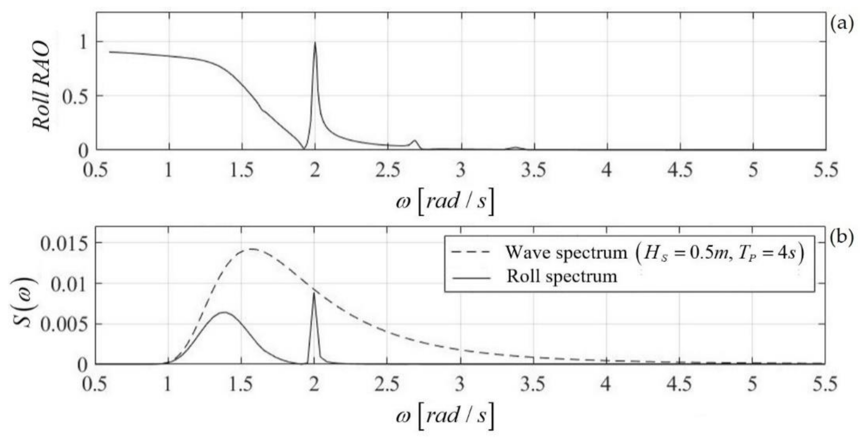
The roll responses calculated by the present model, as discussed in the previous section, were used to evaluate the fluctuations of the AOI and the effect on the power output performance of a PV system consisting of panels, with the aforementioned values of tilt (relative to the horizontal deck of the structure) and azimuth angles. Specifically, the roll spectrum was calculated using the RAO of the roll motion (see Figure 7a) of the twin-hull structure using:
S 4 ω = R A O 2 ω k 2 S ω
where the wavenumber k is given by the dispersion relation of water waves for the water depth considered. Based on the calculated roll spectrum, time series of the roll motion ξ 4 t ; H s , T p of the above floating twin-hull structure were simulated, for the considered configuration (structure and coastal environment) and incident waves, characterized by the parameters H s , T p using the random-phase model [30], Chapter 8.2, (see also [31]).
The results were normalized using the value corresponding to calm water (flat horizontal deck of the structure) in the same sea environment, which results in the following definition of the performance index:
P I t = a cos α m + ξ 4 t + b a cos α m + b
where a = D N I and b = D H I + R I for the geographical area and sea environment considered, respectively, and α m is a representative value for the angle of incidence.
As an example, the numerical results concerning the calculated roll response of a floating twin-hull structure of breadth B ( T ) = 20 m at depth h = 30 m with an incident wave spectrum (dashed line) and roll angle spectrum (solid line) of the structure in the case of incident waves of significant wave height H S = 0.5 m and peak period T P = ( 2 π / ω p ) = 4 s are presented in 
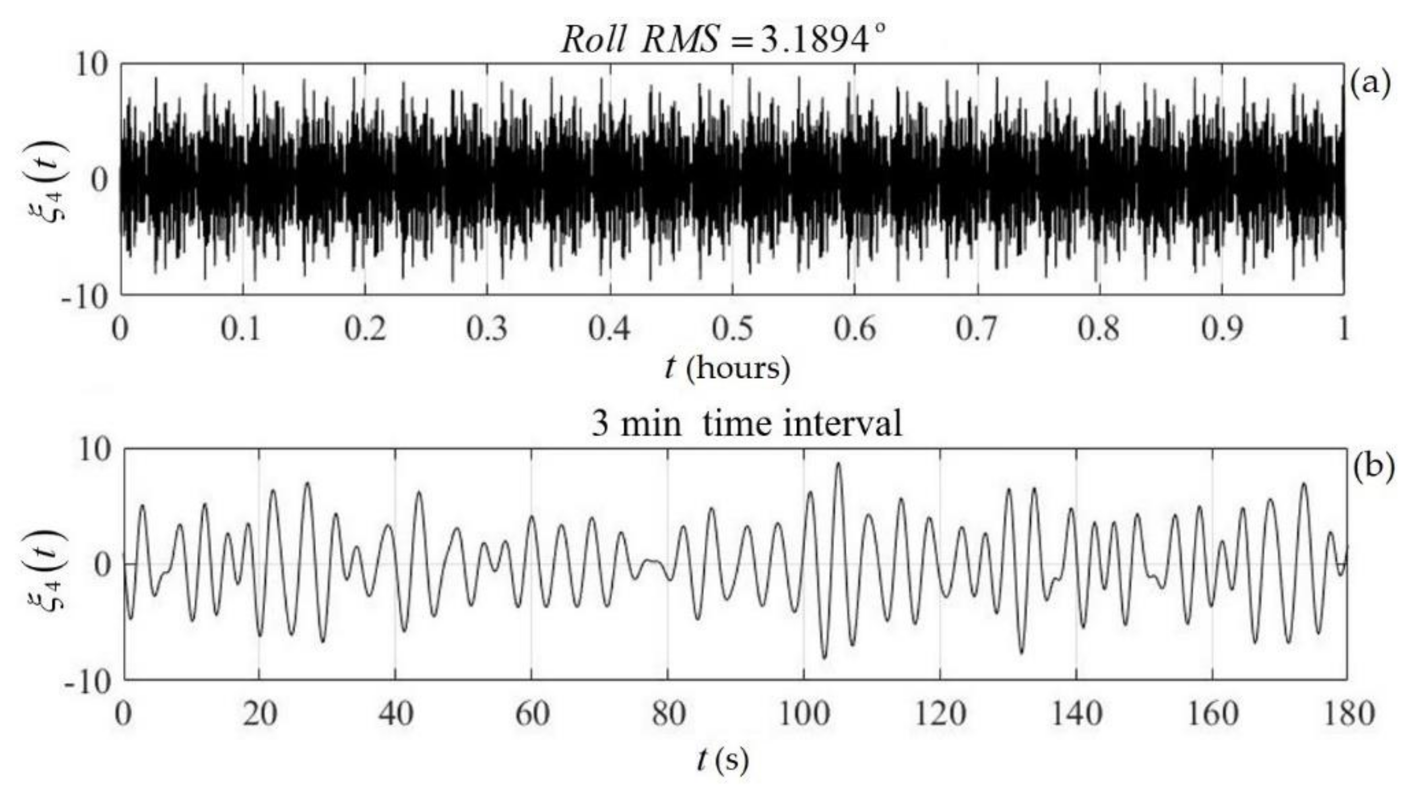
Figure 9. Based on the calculated roll spectrum, the simulated time series of the roll motion of the above floating twin-hull structure for the considered coastal environment and incident waves are shown in 
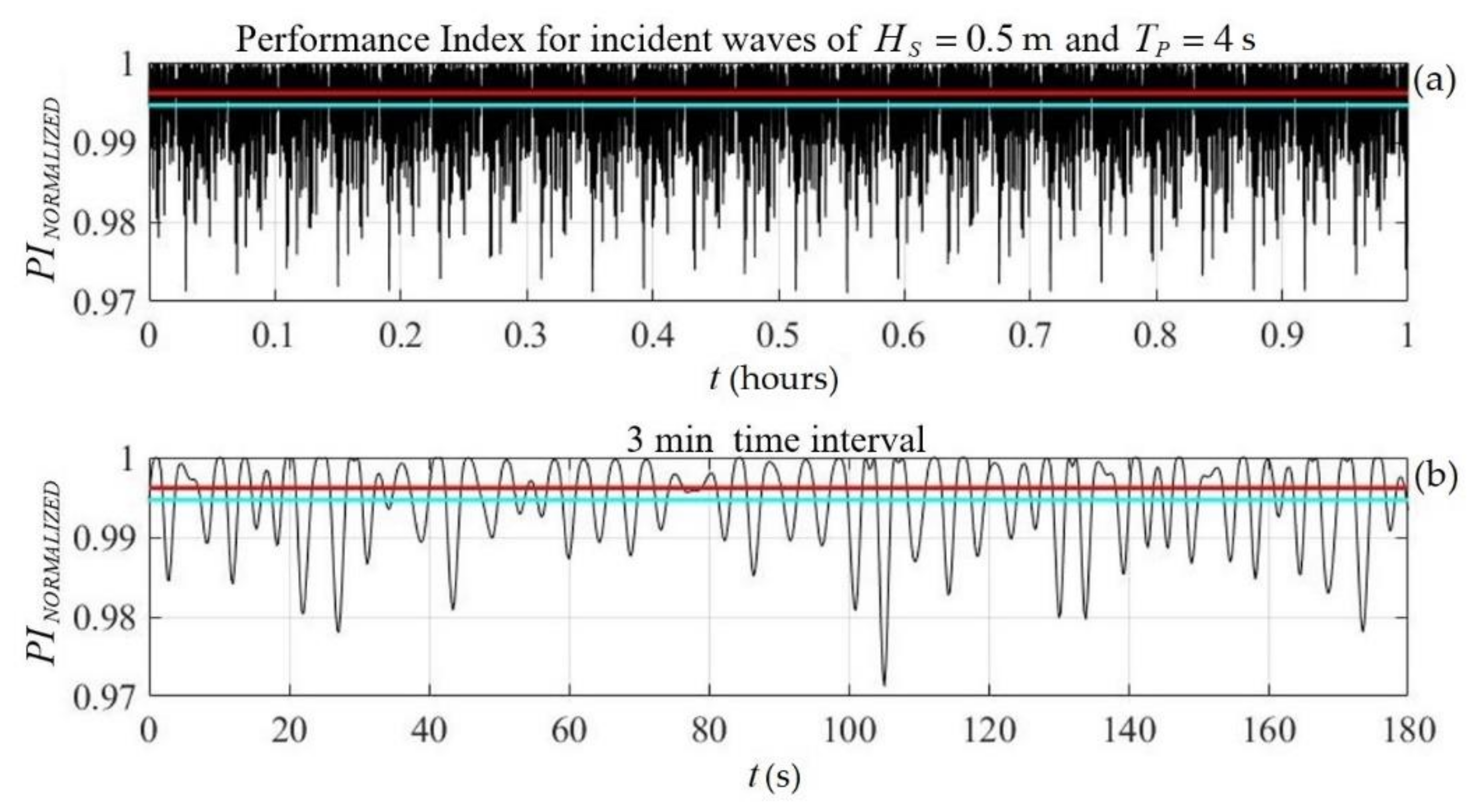
Figure 10 for a time interval of 1 h. Furthermore, in the same figure, a representative small interval of 3 min was obtained using the random-phase model [30,31] for a sea state that was characterized by significant wave height H S = 0.5 m and peak period T P = 4 s , as generated by winds corresponding to the Beaufort scale levels B F = 1 - 2 
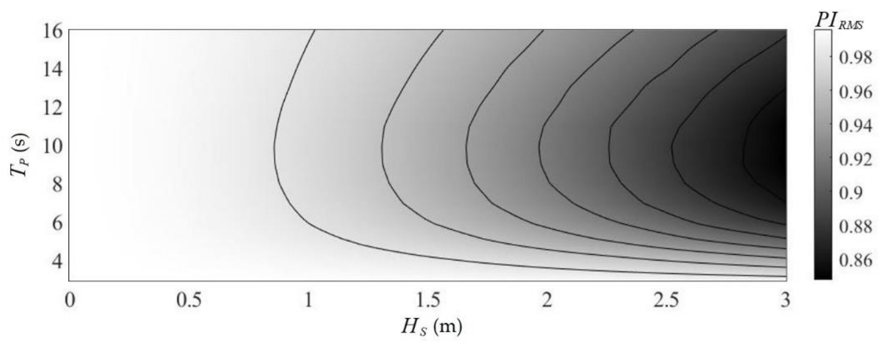
. In this case, indicative results concerning the effect of waves and roll responses of the structure on the performance index are shown in Figure 11, as calculated by Equation (20) using a representative value of the mean angle of incidence α m = 5 ° and omitting, as a first approximation, the effect of diffuse and reflected irradiance components b 0 . The value of the performance index in calm water was P I C A L M = 0.9962 . In the considered case of incident waves, which were characterized by a very low energy content, the R M S value of the estimated performance index dropped to P I R M S = 0.9947 . The latter’s mean value, as well as the corresponding calm-water value, are shown in Figure 11 using cyan and red lines, respectively.

6. Discussion

Following previous works [32,33], concerning the investigation and modeling of marine renewable energy systems, the present method focused on the estimation of the effect of wave-induced responses on the performance index of a twin-hull FPV structure in various sea conditions, as defined by the wave climatology of the offshore–coastal site where the system was deployed. As an example, the results concerning the performance index that is associated with the wave effects (Equation (20)) of the floating twin-hull structure of breadth B ( T ) = 20 m at a water depth h = 30 m that are presented and discussed above are given in Table 1 for wind waves corresponding to the Beaufort scale from B F = 1 (relatively calm sea) to B F = 5 - 6 conditions.
We observe that the effect of roll responses results in fluctuations of the AOI that could cause a significant drop in the performance index as the sea condition changed from calm to moderate and higher severities. A more complete picture of the sea state’s effect on the FPV module’s power output, as estimated using the present method, is shown in Figure 12, indicating its usefulness for supporting the systematic analysis and design of the system, including the offshore structure, as well as the electric production and storage subsystems. Although inevitable fluctuations of the AOI due to waves in offshore PV units reduce the power output, this negative effect could be balanced or even reversed by the cooling effect and other factors resulting from the marine environment, which is a subject that is left to be considered in future work.

7. Conclusions

A BEM model was developed and applied to the hydrodynamic analysis of twin-hull structures in variable bathymetry regions and was used to predict their hydrodynamic responses and their effects concerning the power output of offshore FPV systems. The analysis was restricted to two spatial dimensions for simplicity. After verification of the method with comparisons against data from the literature, the method was systematically applied and the derived numerical results are presented for floating bodies of simple geometry, lying over uniform and sloping seabeds. With the aid of systematic comparisons, the effects of bottom slope on the hydrodynamic characteristics (hydrodynamic coefficients and responses) of the floating bodies were illustrated and discussed. Finally, response data that was simulated for specific sea conditions, characterized by frequency spectra, were considered to describe the incident waves interacting with a floating twin-hull structure, in order to evaluate the effect of wave-induced fluctuations on the power output performance of the floating PV system. The effects of waves on the floating PV performance are presented, indicating significant variations of the performance index ranging from 0 to 15% depending on the sea state. Future work will be directed toward (a) the detailed analysis of wave and wind environmental factors and their effects on the resulting system’s performance, (b) the extension of the model to 3D including 6-DOF wave motion analysis of the floating structures over general bathymetry and evaluation of their performance and (c) a systematic application of the present method to realistic cases that support the optimized design of floating PV modules in specific marine environments.

Author Contributions

Conceptualization, K.B.; methodology, K.B. and A.M; software, A.M. and K.B.; validation, A.M.; writing—original draft preparation, A.M.; writing—review and editing, K.B. and E.R.; visualization, E.R.; supervision, K.B. All authors have read and agreed to the published version of the manuscript.

Funding

This work was supported by the research project DREAM (Dynamics of the Resources and Technological Advance in Harvesting Marine Renewable Energy), funded by the Romanian Executive Agency for Higher Education, Research, Development and Innovation Funding–UEFISCDI, grant number PNIII-P4-ID-PCE-2020-0008.

Acknowledgments

The doctoral studies of A. Magkouris are currently supported by the Special Account for Research Funding (E.L.K.E.) of the National Technical University of Athens (N.T.U.A.) operating in accordance with Law 4485/17 and National and European Community Law.

Conflicts of Interest

The authors declare no conflict of interest.

Abbreviations

AOIAngle of incidence
BCBoundary condition
BEMBoundary element method
BMMetacentric radius
DHIDiffuse horizontal irradiance
DNIDirect normal irradiance
DOFDegree of freedom
DtNDirichlet-to-Neumann
FPVFloating photovoltaic
GMMetacentric height
KBDistance from reference point K to center of buoyancy
KGDistance from reference point K to center of gravity
PIPerformance index
POAPlane of array
PVPhotovoltaic
RAOResponse amplitude operator
RIReflected irradiance
RMSRoot mean square (here of the time series data)
SWLStill-water level

Appendix A. Dirichlet-to-Neumann Operators

By projecting the terms of Equation (5a) on the orthonormal basis, spanned by the normalized eigenfunctions Z ˜ n ( i ) z = Z n ( i ) z / Z n ( i ) , with Z n ( i ) standing for the L 2 norm of each vertical function:
Z n ( i ) = z = h i 0 Z n i x 3 2 d x 3 1 / 2 , i = L , R ,
we obtain
φ p ( L ) x Z ˜ n L x 3 = exp i k 0 L x 2 + C 0 L exp i k 0 L x 2 , n = 0 C n L exp k n L x 2 a , n 1
where f x 3 , g x 3 = x 3 = h a x 3 = 0 f x 3 g x 3   d x 3 . Therefore, the reflection coefficient in the left half-strip D L is equal to
C 0 L = exp i k 0 L x 2 + φ p ( L ) x Z ˜ 0 L x 3 exp i k 0 L x 2 ,   x 2 , x 3 D L
Moreover, by calculating the derivative of Equation (5a) with respect to the unit normal vector n (which is directed opposite to the x 2 direction on D 5 ) and replacing in Equation (6e)
φ p ( L ) x n = i k 0 L exp i k 0 L x 2 C 0 L exp i k 0 L x 2 Z 0 L x 3 +       + n = 1 k n L C n L exp k n L x 2 a Z n L x 3 = T L φ p ( L ) x Q p , x D L ,
and by using Equation (A2), we conclude to
T L φ p ( L ) x = i k 0 L Z ˜ 0 L x 3 φ p ( L ) x Z ˜ 0 L x 3 +       n = 1 k n L Z ˜ n L x 3 φ p ( L ) x Z ˜ n L x 3 ,
where
Q p = 2 i k 0 L exp i k 0 L x 2 Z ˜ 0 L x 3 .  
Similarly, for k = 2 , 3 , 4 , we obtain
φ k ( L ) x n = i k 0 L C 0 L exp i k 0 L x 2 Z 0 L x 3 + + n = 1 k n L C n L exp k n L x 2 a Z n L x 3 = T L φ k ( L ) x Q k ,   x D L .
Using the above results, we obtain T L φ k ( L ) x = T L φ p ( L ) x , k = 2 , 3 , 4 , and Q k = 0 ,   k = 2 , 3 , 4 . Similarly, for the wavefield in the domain D R :
φ p ( R ) x n = i k 0 R C 0 R exp i k 0 R x 2 Z 0 R x 3 +       + n = 1 k n R C n R exp k n R b x 2 Z n R x 3 = T R φ p ( R ) x , x D R .
and thus
T R φ p ( R ) x = i k 0 R Z 0 R x 3 φ k ( R ) x Z ˜ 0 R x 3 +       + n = 1 k n R Z n R x 3 φ k ( R ) x Z ˜ n R x 3 .

References

  1. Trapani, K.; Santafé, M.R. A review of floating photovoltaic installations: 2007-13. Prog. Photovolt. 2014, 23, 524–532. [Google Scholar] [CrossRef] [Green Version]
  2. Grech, M.; Stagno, M.L.; Aquilina, M.; Cadamuro, M.; Witzke, U. Floating Photovoltaic Installation in Maltese Sea Waters. In Proceedings of the 32nd European Photovoltaic Solar Energy Conference and Exhibition, Munich, Germany, 20–24 June 2016. [Google Scholar]
  3. Diendorfer, C.; Haider, M.; Lauermann, M. Performance analysis of offshore solar power plants. Energy Procedia 2014, 49, 2462–2471. [Google Scholar] [CrossRef] [Green Version]
  4. Sukarso, A.P.; Kim, K.N. Cooling Effect on the Floating Solar PV: Performance and Economic Analysis on the Case of West Java Province in Indonesia. Energies 2020, 13, 2126. [Google Scholar] [CrossRef]
  5. Muscat, M. A Study of Floating PV Module Efficiency; Institute for Sustainable Energy, University of Malta: Msida, Malta, 2014. [Google Scholar]
  6. Mei, C.C. The applied Dynamics of Ocean Surface Waves, 2nd ed.; World Scientific: Singapore, 1989. [Google Scholar]
  7. Kuznetsov, N.; Maz’ya, V.; Vainberg, B. Linear Water Waves; Cambridge University Press: Cambridge, UK, 2002. [Google Scholar]
  8. Evans, D.V.; Kuznetsov, C.M. Chapter 4. In Gravity Waves in Water of Finite Depth; Hunt, J.N., Ed.; Computational Mechanics Publications: Southampton, UK, 1997. [Google Scholar]
  9. Takagi, K.; Naito, S.; Hirota, K. Hydrodynamic Forces Acting on a Floating Body in a Harbour of Arbitrary Geometry. In Proceedings of the Third International Offshore and Polar Engineering Conference, Singapore, 6–11 June 1993; Volume 3, pp. 192–199. [Google Scholar]
  10. Ohyama, T.; Tsuchida, M. Expanded mild-slope equations for the analysis of wave-induced ship motion in a harbor. Coast. Eng. 1997, 30, 77–103. [Google Scholar] [CrossRef]
  11. Yeung, R.W. A hybrid integral-equation method for time harmonic free surface flows. In Proceedings of the 1st International Conference on Numerical Ship Hydrodynamics, Gaithersburg, MD, USA, 20–22 October 1975. [Google Scholar]
  12. Nestegard, A.; Sclavounos, P.D. A numerical solution of two-dimensional deep water wave body problems. J. Ship Res. 1984, 28, 48–54. [Google Scholar] [CrossRef]
  13. Drimer, N.; Agnon, Y. A hybrid boundary element method for second-order wave-body interaction. Appl. Ocean Res. 1994, 16, 27–45. [Google Scholar] [CrossRef]
  14. Wehausen, J.; Laitone, E. Surface Waves. In Encyclopedia of Physics, FD III 9; Springer: Berlin, Germany, 1960. [Google Scholar]
  15. Wehausen, J.V. The motion of floating bodies. Annual Rev. Fluid Mech. 1971, 3, 237–268. [Google Scholar] [CrossRef]
  16. Newman, J.N. Marine Hydrodynamics; MIT Press: Cambridge, MA, USA, 1977. [Google Scholar]
  17. Massel, S. Extended refraction-diffraction equations for surface waves. Coast. Eng. 1993, 19, 97–126. [Google Scholar] [CrossRef]
  18. Coddington, E.A.; Levinson, N. Theory of Ordinary Differential Equations; McGraw Hill: New York, NY, USA, 1955. [Google Scholar]
  19. Givoli, D. Non-reflecting boundary conditions. J. Comp. Phys. 1991, 94, 1–29. [Google Scholar] [CrossRef]
  20. Wehausen, J.V. Methods for Boundary-Value Problems in Free-Surface Flows; David Taylor Naval Ship Research and Development Center Rep.: Bethesda, MD, USA, 1974. [Google Scholar]
  21. Kress, R. Linear Integral Equations; Springer: Berlin, Germany, 1989. [Google Scholar]
  22. Katz, J.; Plotkin, A. Low Speed Aerodynamics; McGraw Hill: Singapore, 1991. [Google Scholar]
  23. Belibassakis, K.A. A boundary element method for the hydrodynamic analysis of floating bodies in variable bathymetry regions. Eng. Anal. Bound. Elem. 2008, 32, 796–810. [Google Scholar] [CrossRef]
  24. Lewis, E.V. (Ed.) Principles of Naval Architecture; Society of Naval Architects and Marine Engineers; SNAME: Jersey City, NJ, USA, 1989; Volume III. [Google Scholar]
  25. Drimer, N.; Agnon, Y.; Stiassnie, M. A simplified analytical model for a floating breakwater in water of finite depth. Appl. Ocean Res. 1992, 14, 33–41. [Google Scholar] [CrossRef]
  26. Ohkusu, M. On the Heaving Motion of Two Circular Cylinders on the Surface of a Fluid; Reports of Research Institute for Applied Mechanics; Kyushu University: Kyushu, Japan, 1969. [Google Scholar]
  27. Rhee, K.P. Investigation of the Effect of Water Depths on Two-dimensional Hydrodynamic Coefficients for Twin-Hull Sections. J. Soc. Nav. Archit. Korea 1982, 19, 39–45. [Google Scholar]
  28. Dabssi, N.; Chagdali, M.; Hémon, A. Hydrodynamic Coefficients and Forces on Multihulls in Shallow Water with Constant or Variable Depth. Transport 2008, 23, 245–252. [Google Scholar] [CrossRef]
  29. Dörenkämper, M.; Wahed, A.; Kumar, A.; De Jong, M.; Kroon, J.; Reindl, T. The cooling effect of floating PV in two different climate zones: A comparison of field test data from the Netherlands and Singapore. Sol. Energy 2021, 214, 239–247. [Google Scholar] [CrossRef]
  30. Goda, Y. Random Seas and Design of Maritime Structures; World Scientific: Singapore, 2000. [Google Scholar]
  31. Ochi, M.K. Ocean Waves; The stochastic approach; Cambridge University Press: Cambridge, UK, 1998. [Google Scholar]
  32. Belibassakis, K.; Bonovas, M.; Rusu, E. A Novel Method for Estimating Wave Energy Converter Performance in Variable Bathymetry Regions and Applications. Energies 2018, 11, 2092. [Google Scholar] [CrossRef] [Green Version]
  33. Bonovas, M.; Belibassakis, K.; Rusu, E. Multi-DOF WEC Performance in Variable Bathymetry Regions Using a Hybrid 3D BEM and Optimization. Energies 2019, 12, 2108. [Google Scholar] [CrossRef] [Green Version]
Figure 1. Geometric configuration of the 2D problem.
Energies 14 05979 g001
Figure 2. Amplitude ratios for heave and sway for a twin-hull floating structure with semicircle hull cross-sections 2 P / R = 3 ,   h / R = .
Energies 14 05979 g002
Figure 3. Sway and heave radiation fields for 2 P / R = 3 ,   h = λ / 2 and   ω 2 R / g = 1 . (a,b) Real and imaginary part of the normalized sway field φ 2 x and corresponding free-surface elevation. (c,d) Real and imaginary part of the normalized heave field φ 3 x and corresponding free-surface elevation.
Energies 14 05979 g003
Figure 4. Added mass and damping coefficient of heave, for a twin-hull floating structure of semicircle hull cross sections 2 P / R = 3 ,   h / R = 2 .
Energies 14 05979 g004
Figure 5. Outline of the modeled configuration and basic dimensions.
Energies 14 05979 g005
Figure 6. (a) Floating body and domains of transmission ( B ( T ) / h = 2 / 3 ,   B ( H ) / h = T / h = 1 / 10 ). (b) Hydrodynamic forces F ˜ k ,   k = 2 , 3 . (c,d) RAOs in sway and heave motions, respectively. (e,f) Hydrodynamic coefficients A 22 , B 22 and A 33 , B 33 , respectively. All quantities were plotted vs. the non-dimensional wavelength λ / h , where h denotes the average water depth.
Energies 14 05979 g006
Figure 7. (a) RAO in roll motion. (b) Hydrodynamic moment F ˜ 4 . (c,d) Hydrodynamic coefficients A 44 , B 44 and A 24 , B 24 , respectively. All quantities are plotted vs. the non-dimensional wavelength λ / h , where h denotes the average water depth.
Energies 14 05979 g007
Figure 8. (a) Real and (b) Imaginary Part of the total complex wave potential and corresponding free surface elevation for a twin-hull floating structure of breadth B = 20 m and three considered cases of bottom slope 0, 10 and 20% in an environment with a mean depth of h = 30 m in the case of an incident wave of wavelength λ / h = 2.4 and amplitude A = 1.5 m .
Energies 14 05979 g008
Figure 9. (a) Roll response of the floating twin-hull structure of breadth B = 20 m at a mean depth h = 30 m. (b) Incident wave spectrum (dashed line) and roll angle spectrum (solid line) of the structure in the case of incident waves with a significant wave height H S = 0.5 m and a peak period T P = 4 s .
Energies 14 05979 g009
Figure 10. Simulated time series of the floating twin-hull structure’s roll motion. Total breadth B ( T ) = 20 m at a depth h = 30 m in the case of incident waves with a significant wave height equal to H S = 0.5 m and a peak period T P = 4 s . (a) A 1 h long time series and (b) indicative roll motion over a 3 min long interval.
Energies 14 05979 g010
Figure 11. Performance Index of FPV on the floating twin hull structure of breadth B ( T ) = 20 m at a depth h = 30 m in the case of incident waves with a significant wave height H S = 0.5 m and a peak period T P = 4 s . Roll motion time series (a) in a 1 h long time interval and (b) in an indicative 3 min long time interval.
Energies 14 05979 g011
Figure 12. Contour map of the normalized performance index as a function of the prevailing sea state (significant wave height H S and peak period T P ).
Energies 14 05979 g012
Table 1. Performance indexes for different sea conditions.
BFSea Condition H S m T P s P I R M S
1–21–20.540.9947
33160.9771
4–54280.9203
5–64–5390.8475
Publisher’s Note: MDPI stays neutral with regard to jurisdictional claims in published maps and institutional affiliations.

