Abstract
Fibromyalgia is a medical condition characterized by widespread muscle pain and tenderness and is often accompanied by fatigue and alteration in sleep, mood, and memory. Poor sleep quality and fatigue, as prominent characteristics of fibromyalgia, have a direct impact on patient behavior and quality of life. As such, the detection of extreme cases of sleep quality and fatigue level is a prerequisite for any intervention that can improve sleep quality and reduce fatigue level for people with fibromyalgia and enhance their daytime functionality. In this study, we propose a new supervised machine learning method called Learning Using Concave and Convex Kernels (LUCCK). This method employs similarity functions whose convexity or concavity can be configured so as to determine a model for each feature separately, and then uses this information to reweight the importance of each feature proportionally during classification. The data used for this study was collected from patients with fibromyalgia and consisted of blood volume pulse (BVP), 3-axis accelerometer, temperature, and electrodermal activity (EDA), recorded by an Empatica E4 wristband over the courses of several days, as well as a self-reported survey. Experiments on this dataset demonstrate that the proposed machine learning method outperforms conventional machine learning approaches in detecting extreme cases of poor sleep and fatigue in people with fibromyalgia.
1. Introduction
Fibromyalgia is medical condition characterized by widespread muscle pain and tenderness that is typically accompanied by a constellation of other symptoms, including fatigue and poor sleep [1,2,3,4,5,6,7,8,9]. Poor sleep, which is a cardinal characteristic of fibromyalgia, is strongly related to greater pain and fatigue, and lower quality of life [10,11,12,13,14,15,16]. As a result, any intervention that can improve sleep quality may enhance daytime functionality and reduce fatigue in people with fibromyalgia.
Studies of sleep in fibromyalgia often rely on self-reported measures of sleep or polysomnography. While easy to administer, self-reported measures of sleep demonstrate limited reliability and validity in terms of their correspondence with objective measures of sleep. In contrast, polysomnography is considered the gold standard of objective sleep measurement; however, it is expensive, difficult to administer, especially on a large scale, and may lack ecological validity. Autonomic nervous system (ANS) imbalance during sleep has been implicated as a mechanism underlying unrefreshed sleep in fibromyalgia. ANS activity can be assessed unobtrusively through ambulatory measures of heart rate variability (HRV) and electrodermal activity (EDA) [17,18]. Wearable devices such as the Empatica E4 are able to directly, continuously, and unobtrusively measure autonomic functioning such as EDA and HRV [19,20,21,22].
In the literature, there are few studies in which machine learning methods are used for classification or prediction of conditions related to fibromyalgia, none of which use physiological signals. A recent survey paper [23] summarizes various types of machine learning methods that have been used in pain research, including fibromyalgia. Previously, using data from 26 individuals (14 individuals with fibromyalgia and 12 healthy controls), the relative performance of machine learning methods for classification of individuals with and without pain using neuroimaging and self-reported data have been compared [24]. In another study using MRI images of 59 subjects, support vector machine (SVM) and decision tree models were used to first distinguish healthy control patients from those with fibromyalgia or chronic fatigue syndrome, and then differentiate fibromyalgia from chronic fatigue syndrome [25]. In [26], an SVM trained on fMRI images was used to distinguish fibromyalgia patients from healthy controls. The combination of fMRI with multivariate pattern analysis has also been investigated in classifying fibromyalgia patients, rheumatoid arthritis patients and healthy controls [27]. Psychopathologic features within an ADABoost classifier have also been employed for classification of patients with fibromyalgia and arthritis [28]. In another recent work [29], secondary analysis of gene expression data from 28 patients with fibromyalgia and 19 healthy controls was used to distinguish between these two groups.
In this study our immediate interest is to predict extreme cases of fatigue and poor sleep in people with fibromyalgia. For such an analysis, we use self-reported quality of sleep and fatigue severity, continuously collected data from the Empatica E4, to measure autonomic nervous system activity during sleep (Section 2). These signals are preprocessed to remove noise and other artifacts as described in Section 3.1. After preprocessing, a number of mathematical features are extracted, including various statistics, signal characteristics, and HRV features (Section 3.2). Section 4 provides a detailed description of our novel Learning Using Concave and Convex Kernels (LUCCK) machine learning method. This model, along with other conventional machine learning methods, were trained on the extracted features and used to predict extreme cases of poor sleep and fatigue, with our method yielding the best results (Section 5).
We believe this analytical framework can be readily extended to outpatient monitoring of daytime activity, with applications to assessing extreme levels of fatigue and pain, such as those experienced by patients undergoing chemotherapy.
2. Dataset
The data used for this study was collected from a group of 20 adults with fibromyalgia and consists primarily of a set of signals recorded by an Empatica E4 wristband over the course of seven days (removing 1 h/day for charging/download). Most (80%) participants were female with mean age = 38.79 (min-max = 18–70 years). Of a possible 140 nights of sleep data, the sample had data for 119 (85%) nights. In this dataset, 19.9% of heartbeats were missing due to noisy signals or failure of the Empatica E4 in detecting beats. Data were divided into 5-min windows for HRV analysis; windows with more than 15% missing peaks were eliminated. This led to the exclusion of 30.9% of the windows. The signals used in this analysis are each patient’s blood volume pulse (BVP), 3-axis accelerometer, temperature, and EDA. In addition to these recordings, each subject self-reported his or her wake and sleep times, as well as self-assessed his or her level of fatigue and quality of sleep every morning. These data are labeled by self-reported quality of sleep (1 to 10, 1 being the worst) and level of fatigue (from 1 to 10, 10 indicating the highest level of fatigue).
3. Signal Processing: Preprocessing, Filtering, and Feature Extraction
The schematic diagram of Figure 1 represents our approach to analyzing the BVP and accelerometer signals in the fibromyalgia dataset. During preprocessing, we remove noise from the input signals and format them for future processing (via the Epsilon Tube filter). Once the BVP and accelerometer signals are fully processed, they along with the EDA and temperature signals can then be analyzed and features can be extracted, which in turn leads to the application of machine learning. The final output is a prediction model to which new data can be fed.
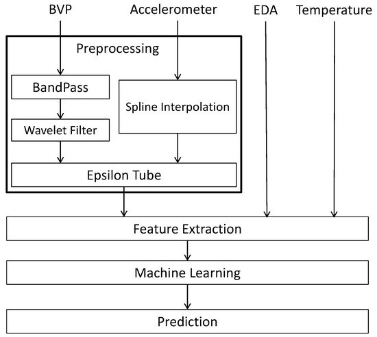
Figure 1.
Schematic Diagram of the Proposed Processing System for BVP, accelerometer, EDA and temperature signals.
3.1. Preprocessing
To begin, the raw signals are extracted per patient according to his or her reported wake and sleep times. These are then split into two groups: awake and asleep. For each patient and day, the awake data is paired with the following night’s data and ensuing morning’s self-assessed level of fatigue and quality of sleep.
Our approach to preprocessing BVP signals consists of a bandpass filter (to remove both the low-frequency components and the high-frequency noise), a wavelet filter (to help reduce motion artifacts while maintaining the underlying rhythm), and Epsilon Tube filtering. In order to least perturb the true BVP signal, we chose the Daubechies mother wavelet of order 2 (’db2’) as it closely resembles the periodic shape of the BVP signal. Other wavelets were also considered but ultimately discarded. Once we selected a mother wavelet, we performed an eight-level deconstruction of the input BVP signal. By setting threshold values for each level of detail coefficients (Table 1) and using the results to reconstruct the original signal, we were able to significantly reduce the amount of noise present without compromising the measurement integrity of the underlying physiological values. Utilizing this filter on a number of test cases showed that the threshold values produced consistently useful results regardless of the input, meaning tailored interactions are not required for each signal.

Table 1.
Chosen coefficient thresholds for the 8-level wavelet decomposition.
The accelerometer data was upsampled from 32 Hz to 64 Hz via spline interpolation to match the sampling frequency of the BVP signal. The other signals (temperature and EDA) were left unfiltered. We then use these preprocessed signals as input into our main filtering approach (Epsilon Tube), the output of which is then used for feature extraction (Section 3.2).
After filtering of the BVP signal and interpolation of the accelerometer signal, the Epsilon Tube filter [30] is the final component of the preprocessing stage. As discussed in [30], since the BVP signal (and generally any impedance-plethysmography-based measurements) is very susceptible to motion artifact, reduction of this noise is a crucial part of the filtering process. This method uses the synchronized accelerometer data to estimate the motion artifact of BVP signal while leaving the periodic component intact. Let represent BVP values at time t, A a matrix whose rows are the accelerometer signals, and the vector of Epsilon Tube filter coefficients. Given the tube radius , the error of estimation, i.e., , is zero if the point falls inside the tube
The Epsilon Tube filter is formulated as a constrained optimization problem that can be expressed as
subject to
where N is the length of BVP signal, and are slack variables, is the regularization term and c is a designated parameter that adjusts the trade-off between the two objectives. More information about the Epsilon Tube filter can be found in [30]. Taking both the BVP and accelerometer signals as input, the method assumes periodicity in the BVP signal and looks for a period of inactivity at the beginning of the data to use as a template for the rest of the signal. To achieve this, the calmest section of the accelerometer signal (as determined by the longest stretch during which the values never exceed one standard deviation from the mean of the signal) is found. The signal is then shifted so this period of inactivity is at the beginning, and the BVP signal is also shifted to ensure the timestamps remain aligned. The shifted signals are then fed into the Epsilon Tube algorithm, and the resulting output is used for feature extraction.
3.2. Feature Extraction
Once the BVP and accelerometer signals are processed, the full signal set is used for feature extraction. There are 91 features extracted from each of the following signals:
- Denoised (filtered) BVP signal, i.e., the output of the Epsilon Tube algorithm, with sampling frequency of 64 Hz.
- Low-band, mid-band, and high-band pass filters applied to the denoised BVP signal.
- Interpolated accelerometer signal, from 32 HZ to 64 Hz.
- Tube sizes from the Epsilon Tube filtering method, another output of the Epsilon Tube algorithm that has the time-varying tube size signal.
- Temperature signal, with sampling frequency of 4 Hz.
- EDA signal, with sampling frequency of 4 Hz.
- The calculated breaths per minute (BPM) signal based on the denoised BVP signal.
- The calculated HRV signal based on the denoised BVP signal.
The extracted features are listed in Table 2. These are extracted from both the awake and the sleep signals, resulting in a full feature set consisting of 182 features. When feature selection is performed using Weka’s information gain algorithm [31] on the first four subjects, the only feature ranked consistently near the top is the average of the BVP signal after being run through a mid-band bandpass filter.
Table 2.
The list of features extracted from all signals.
4. Machine Learning: Learning Using Concave and Convex Kernels
The final step in the analysis pipeline is the creation of a model that can be used to predict the extreme cases of quality of sleep or level of fatigue for people with fibromyalgia. As detailed in Section 5, in addition to testing a number of conventional machine learning methods, we tested a novel supervised machine learning called Learning Using Concave and Convex Kernels (LUCCK). A key factor in the classification of complex data is the ability of the machine learning algorithm to use vital, feature-specific information to detect settled and complex patterns of changes in the data. The LUCCK method does this by employing similarity functions (defined below) to capture and quantify a model for each of the features separately. The similarity functions are parametrized so that the concavity or convexity of the function within the feature space can be modified as desired. Once the similarity functions and attendant parameters are chosen, the model uses this information to reweight the importance of each feature proportionally during classification.
4.1. Notation
In this section, is a real-valued vector of features such that , and is a real-valued (scalar) feature. Throughout this section, we consider d classes, n features and m (data) samples; also the indexes ; ; and are used for classes, features and samples respectively. Additionally, refers to samples in class .
4.2. Classification Using a Similarity Function
An instructive model for comparison to the Learning Using Concave and Convex Kernels method is the k-nearest neighbors algorithm [33,34,35] and weighted k-nearest neighbors algorithm [36]. In k-nearest neighbors, a test sample is classified by comparing it to the k nearest training samples in each class. This can make the classification sensitive to a small subset of samples. Instead, LUCCK classifies test data by comparing it to all training data, properly weighted according to their distance to , which is determined by a similarity function. One major difference between LUCCK and weighted k-nearest neighbors is that our approach is based on a similarity function that can be highly non-convex. A fat-tailed (relative to a Gaussian) distribution is more realistic for our data, given that there is a small but non-negligible chance that large errors may occur during measurement, resulting in a large deviation in the values of one or more of the features. The LUCCK method allows for large deviations in a few of the features with only a moderate penalty. Methods based on convex notions of similarity or distance (such as the Mahalanobis distance) are unable to deal adequately with such errors.
Suppose that the feature space is comprised of real-valued vectors . A similarity function is a function that measures the closeness of to the origin, and satisfies the following properties:
- for all ;
- for all ;
- if is non-zero and .
The value measures the closeness between the vectors and . Using the similarity function , a classification algorithm can be created as follows:
The set of training data C is a subset of and is a disjoint union of d classes: . Let be the cardinality of C and define for all k so that . To measure the proximity of a feature vector to a set Y of training samples, we simply add the contributions of each of the elements in Y:
A vector is classified in class , where k is chosen such that is maximal. This classification approach can also be used as the maximum a posteriori estimation (details can be found in Appendix A).
4.3. Choosing the Similarity Function
The function has to be chosen carefully. Let be defined as the product
where and only depends on the i-th feature. The function is again a similarity function satisfying the properties for all , and whenever . After normalization, the can be considered as probability density functions. As such, the product formula can be interpreted as instance-wise independence for the comparison of training and test data. In the naive Bayes method, features are assumed to be independent globally [37]. Summing over all instances in the training data allows for features to be independent in our model.
Next we need to choose the functions . One could choose , so that
is a Gaussian kernel function (up to a scalar). However, this does not work well in practice:
- One or more of the features is prone to large errors —The value of is close to 0 even if and only differ significantly in a few of the features. This choice of is therefore very sensitive to small subsets of bad features.
- The curse of dimensionality—For the training data to properly represent the probability distribution function underlying the data, the number of training vectors should be exponential in n, the number of features. In practice, it usually is much smaller. Thus, if is a test vector in class , there may not be a training vector in for which is not small.
Consequently, let
for some parameters . The function can behave similarly to the Cauchy distribution. This function has a “fat tail": as the rate that goes to 0 is much slower than the rate at which goes to 0. We have
The function Q has a finite integral if for all i, though this is not required. Three examples of this function can be found in Appendix B.
4.4. Choosing the Parameters
Values for the parameters and must be chosen to optimize classification performance. The value of is the most sensitive to changes in x when
is maximal. An easy calculation shows that this occurs when . Since the value directly controls the wideness of ’s tail, it is reasonable to choose a value for that is close to the standard deviation of the i-th feature. Suppose that the set of training vectors is
where for all j.
Let , where
be the standard deviation of the i-th feature. Let
where is some fixed parameter.
Next we choose the parameters . We fix a parameter that will be the average value of . If we use only the i-th feature, then we define
for any set Y of feature vectors. For in the class , gives the average value of over . The quantity measures how much closer is to samples in the class than to vectors in the set C of all feature vectors except itself. This value measures how well the i-th feature can classify as lying in as opposed to some other class. If we sum over all and ensure that the result is non-negative we obtain
The can be chosen so that they have the same ratios as and sum up to :
In terms of complexity, if n is the number of features and m is the number of training samples then the complexity of the proposed method would be .
4.5. Reweighting the Classes
Sometimes a disproportionate number of test vectors are classified as belonging to a particular class. In such cases one might get better results after reweighting the classes. The weights can be chosen so that all are greater than or equal to 1. If p is a probability vector, then we can reweight it to a vector
where
If the output of the algorithm consists of the probability vectors the algorithm can be modified so that it yields the output . A good choice for the weights can be learned by using a portion of the training data. To determine how well a training vector can be classified using the remaining training vectors in , we define
The value is an estimate for the probability that lies in the class , based on all feature vectors in C except itself. We consider the effect of reweighting the probabilities , by
If lies in the class , then the quantity
measures how badly is misclassified if the reweighting is used. The total amount of misclassification is
We would like to minimize this over all choices of . As this is a highly nonlinear problem, making optimization difficult, we instead minimize
instead. This minimization problem can be solved using linear programming, i.e., by minimizing the quantity
for the variables and new variables under the constraints that
and
for all k and j with and .
5. Experiments
In this section, the performance of LUCCK is first compared with other common machine learning methods using four conventional datasets, after which its performance on the fibromyalgia dataset is evaluated.
5.1. UCI Machine Learning Repository
In this set of experiments, LUCCK in compared to some well-known classification methods on a number of datasets downloaded from the University of California, Irvine (UCI) Machine Learning Repository [38]. Each method was tested on each dataset using 10-fold cross-validation, with the average performance and execution time across all folds provided in Table 3. Table 4 contains the average values for accuracy and time across all four datasets.
Table 3.
Comparison of our proposed method (LUCCK) with other machine learning methods in terms of accuracy and running time, averaged over 10 folds.
Table 4.
Model accuracy with standard deviation and execution time for each model, averaged across the four UCI datasets.
5.2. Fibromyalgia Dataset
In this study, we have created a model that can be used to predict the quality of sleep or level of fatigue for people with fibromyalgia. The labels are self-assessed scores ranging from 1 to 10. Attempts to develop a regression model showed less promise than the results from a binary split. The most likely reason for this failure of the linear regression model is the nature of self-reported scores, especially those related to patient assessment of their level of pain. This fact is primarily due to the differences in individual levels of pain-tolerance. In previous studies [39,40], proponents of neural "biomarkers" argued that self-reported scores are unreliable, making objective markers of pain imperative. In another study [24], self-reported scores were found to be reliable only for extreme cases of pain and fatigue. Consequently, in this study, binary classification of extreme cases of fatigue and poor sleep is investigated. In this situation, a cutoff value is selected: patients that chose a value less than the threshold are placed in one group, while those that chose a value above the threshold are placed in another. As such, the values >8 are chosen for extreme cases of fatigue, and the values <4 are chosen for extreme cases of poor sleep quality. In this way, binary classifications are possible (>8 vs. <8 for fatigue and >4 vs. <4 for sleep). Using the extracted feature set, machine learning algorithms are applied and tested using 10-fold cross-validation. This is done in a way so as to prevent the data from any one patient being in multiple folds: all of a given patient’s data are including entirely in a single fold. In addition, in order to address possibly imbalanced data during fold creation, random undersampling is performed to ensure the ratio between the two classes is not less than 0.3 (this rate is chosen since the extreme cases are at most 30 percent of the [1,10] interval of self-reported scores). This prevents the methods from developing a bias towards the larger class.
5.2.1. Results with Conventional Machine Learning Methods
A number of conventional machine learning models listed in Table 5 were applied to the extracted data in this study. As can be seen, many major machine learning methods were tested. For each of these methods, various configurations were tested, and the best sets of parameters were chosen using cross-validation (hyperparameter optimization). For instance, we used the combination of AdaBoost with different types of standard methods such as Decision Stump and Random Forest in order to explore the possibility of improving the performance of these methods via boosting. The k-nearest neighbor method with was used in this experiment. For the weighted k-nearest neighbor method [36], the inversion kernel (inverse distance weights) with resulted in the best performance. For the Neural Network algorithm, the Weka (Waikato Environment for Knowledge Analysis) [41] multilayer perceptron with two hidden layers was used. The results of using these machine learning approaches for prediction of extreme sleep quality (cutoff of 4) and fatigue level (cutoff of 8) are presented in Table 5. As shown in this table, the AdaBoost method based on random forest yielded the best results for quality of sleep (based on area under the receiver operating characteristic curve, or AUROC). For level of fatigue, the neural network was the best performing model.
Table 5.
Results of conventional machine learning methods.
5.2.2. Results with Our Machine Learning Method: Machine Learning Using Concave and Convex Kernels
In addition to the aforementioned conventional methods, we also used our machine learning approach that resulted in superior performance compared to the standard machine learning methods discussed above. Recall that in the Learning Using Concave and Convex Kernels algorithm, test data is classified by comparing it to all training data, properly weighted according to information extracted from each of the features (see Section 4 for further details). The results of applying our method to fibromyalgia are presented in Table 5, with cutoff values of 4 and 8 for quality of sleep and level of fatigue, respectively. As can be seen, LUCCK was able to vastly outperform other models on the fatigue outcome; however, the improvement on sleep outcome was not significant. This disparity is likely due to the different feature spaces for the sleep and fatigue outcomes. In general, the feature space for fatigue is significantly more dispersed, due to there being more samples (during daytime) and also that daytime activity negatively affects the signal quality, increasing dispersion. In contrast, signals (and their associated features) recorded during sleep are of better quality. This leads to the better prediction result for sleep in all methods used. Our proposed LUCCK algorithm can ameliorate the nature of the fatigue feature space, as it is specifically designed to reduce the effect of training data for which there is a large deviation from test data. As such, LUCCK was able to vastly outperform other models on the fatigue outcome. We should note that while the cohort size in this study seems to be limited, the continuous recording of physiological signals for seven days and nights created a comprehensive dataset. Additionally, similar to k-NN and its weighted version (and unlike SVM and neural network models), LUCKK can be trained even with few samples, which is one advantage of the proposed algorithm.
6. Conclusions and Discussion
In this study we primarily focused on prediction of the extreme cases of fatigue and poor sleep. As such, we have created preprocessing/conditioning methods that have the ability to improve the quality of parts of the signals with low quality due to motion artifact and noise. In addition, we identified a set of mathematical features that are important in extracting patterns from physiological signals that can distinguish poor and good clinical outcomes for applications such as fibromyalgia. Additionally, we showed that our proposed machine learning method outperformed the standard methods in predicting the outcomes such as fatigue and sleep quality. Generally, our proposed framework (preprocessing, mathematical features, and proposed machine learning method) can be employed in any study that involves prediction using BVP, HRV and EDA signals.
The epsilon tube filter is covered by US Patent 10,034,638, for which Kayvan Najarian is a named inventor.
Author Contributions
Conceptualization, H.D.; Data curation, C.B. and S.A.; Formal analysis, E.S.; Funding acquisition, H.I. and K.N.; Supervision, A.K. and K.N.; Writing—original draft, E.S.; Writing—review & editing, J.G. and K.N.
Funding
This research was funded by Care Progress LLC through National Science Foundation grant number 1562254.
Conflicts of Interest
The authors declare no conflict of interest.
Abbreviations
The following abbreviations are used in this manuscript:
| LUCCK | Learning Using Concave and Convex Kernels |
| BVP | Blood Volume Pulse |
| EDA | Electrodermal Activity |
| ANS | Autonomic Nervous System |
| HRV | Heart Rate Variability |
| FFT | Fast Fourier transform |
| BPM | Breaths Per Minute |
| AUROC | Area Under Receiver Operating Characteristic Curve |
Appendix A Classification as Maximum a Posteriori Estimation
The classification approach suggested in Section 4.2 can also be viewed in terms of probability density functions. Suppose that with . The function
is therefore a probability density function. This probability density function is an estimation for the probability distribution from which the training data were taken.
We have
where
is a probability density function for the training data in class for and is the probability that a randomly chosen training vector lies in . can be considered as a mixture of the probability density functions . Suppose that is taken from the distribution with probability , then the distribution for is . Given the outcome , the probability that it was taken from the distribution is
This shows that the classifying scheme is the maximum a posteriori estimation. Instead of classifying a feature vector, the probability vector
can be given as output. The formula
is well-formed, even if does not have a finite integral, which may be the case in some examples.
Appendix B. Examples
Example A1.
Suppose that there is only one feature, i.e., , then can be defined as
whose graph at various values of θ and λ is depicted in Figure A1:


Figure A1.
with for (blue curves) and (red curve).
Figure A1.
with for (blue curves) and (red curve).
As goes to zero, the function converges to the normal distribution (the red curve in Figure A1).
Example A2.
Suppose that , then is defined as
with . is depicted in Figure A2 at various level curves for , with .


Figure A2.
with .
Figure A2.
with .
The Equation is a closed curve. Such a curve can be thought of as the set of all points that have a given distance to the origin. We observe that for , the neighborhood
of the origin is convex, but for it is not.
Example A3.
Consider the case when and , , and , then is defined as
is depicted in Figure A3 at various level curves for , with .


Figure A3.
with .
Figure A3.
with .
For small values of , the function Q is equally sensitive to and . However, if is large, then Q is more sensitive to .
References
- Moldofsky, H. The significance of dysfunctions of the sleeping/waking brain to the pathogenesis and treatment of fibromyalgia syndrome. Rheumatic Dis. Clin. 2009, 35, 275–283. [Google Scholar] [CrossRef]
- Moldofsky, H. The significance of the sleeping–waking brain for the understanding of widespread musculoskeletal pain and fatigue in fibromyalgia syndrome and allied syndromes. Joint Bone Spine 2008, 75, 397–402. [Google Scholar] [CrossRef] [PubMed]
- Horne, J.; Shackell, B. Alpha-like EEG activity in non-REM sleep and the fibromyalgia (fibrositis) syndrome. Electroencephalogr. Clin. Neurophysiol. 1991, 79, 271–276. [Google Scholar] [CrossRef]
- Burns, J.W.; Crofford, L.J.; Chervin, R.D. Sleep stage dynamics in fibromyalgia patients and controls. Sleep Med. 2008, 9, 689–696. [Google Scholar] [CrossRef]
- Belt, N.; Kronholm, E.; Kauppi, M. Sleep problems in fibromyalgia and rheumatoid arthritis compared with the general population. Clin. Expe. Rheumatol. 2009, 27, 35. [Google Scholar]
- Landis, C.A.; Lentz, M.J.; Rothermel, J.; Buchwald, D.; Shaver, J.L. Decreased sleep spindles and spindle activity in midlife women with fibromyalgia and pain. Sleep 2004, 27, 741–750. [Google Scholar] [CrossRef]
- Stuifbergen, A.K.; Phillips, L.; Carter, P.; Morrison, J.; Todd, A. Subjective and objective sleep difficulties in women with fibromyalgia syndrome. J. Am. Acad. Nurse Pract. 2010, 22, 548–556. [Google Scholar] [CrossRef] [PubMed]
- Theadom, A.; Cropley, M.; Parmar, P.; Barker-Collo, S.; Starkey, N.; Jones, K.; Feigin, V.L.; BIONIC Research Group. Sleep difficulties one year following mild traumatic brain injury in a population-based study. Sleep Med. 2015, 16, 926–932. [Google Scholar] [CrossRef]
- Buskila, D.; Neumann, L.; Odes, L.R.; Schleifer, E.; Depsames, R.; Abu-Shakra, M. The prevalence of musculoskeletal pain and fibromyalgia in patients hospitalized on internal medicine wards. Semin. Arthritis Rheum. 2001, 30, 411–417. [Google Scholar] [CrossRef] [PubMed]
- Theadom, A.; Cropley, M.; Humphrey, K.L. Exploring the role of sleep and coping in quality of life in fibromyalgia. J. Psychosom. Res. 2007, 62, 145–151. [Google Scholar] [CrossRef]
- Theadom, A.; Cropley, M. This constant being woken up is the worst thing–experiences of sleep in fibromyalgia syndrome. Disabil. Rehabil 2010, 32, 1939–1947. [Google Scholar] [CrossRef] [PubMed]
- Stone, K.C.; Taylor, D.J.; McCrae, C.S.; Kalsekar, A.; Lichstein, K.L. Nonrestorative sleep. Sleep Med. Rev. 2008, 12, 275–288. [Google Scholar] [CrossRef]
- Harding, S.M. Sleep in fibromyalgia patients: Subjective and objective findings. Am. J. Med. Sci. 1998, 315, 367–376. [Google Scholar] [PubMed]
- Landis, C.A.; Frey, C.A.; Lentz, M.J.; Rothermel, J.; Buchwald, D.; Shaver, J.L. Self-reported sleep quality and fatigue correlates with actigraphy in midlife women with fibromyalgia. Nurs. Res. 2003, 52, 140–147. [Google Scholar] [CrossRef]
- Fogelberg, D.J.; Hoffman, J.M.; Dikmen, S.; Temkin, N.R.; Bell, K.R. Association of sleep and co-occurring psychological conditions at 1 year after traumatic brain injury. Arch. Phys. Med Rehabil. 2012, 93, 1313–1318. [Google Scholar] [CrossRef]
- Towns, S.J.; Silva, M.A.; Belanger, H.G. Subjective sleep quality and postconcussion symptoms following mild traumatic brain injury. Brain Injury 2015, 29, 1337–1341. [Google Scholar] [CrossRef] [PubMed]
- Trinder, J.; Kleiman, J.; Carrington, M.; Smith, S.; Breen, S.; Tan, N.; Kim, Y. Autonomic activity during human sleep as a function of time and sleep stage. J. Sleep Res. 2001, 10, 253–264. [Google Scholar] [CrossRef]
- Baharav, A.; Kotagal, S.; Gibbons, V.; Rubin, B.; Pratt, G.; Karin, J.; Akselrod, S. Fluctuations in autonomic nervous activity during sleep displayed by power spectrum analysis of heart rate variability. Neurology 1995, 45, 1183–1187. [Google Scholar] [CrossRef]
- Sano, A.; Picard, R.W.; Stickgold, R. Quantitative analysis of wrist electrodermal activity during sleep. Int. J. Psychophysiol. 2014, 94, 382–389. [Google Scholar] [CrossRef]
- Sano, A.; Picard, R.W. Comparison of sleep-wake classification using electroencephalogram and wrist-worn multi-modal sensor data. In Proceedings of the 36th Annual International Conference of the IEEE Engineering in Medicine and Biology Society, Chicago, IL, USA, 26–30 August 2014; Volume 2014, p. 930. [Google Scholar]
- Sano, A.; Picard, R.W. Recognition of sleep dependent memory consolidation with multi-modal sensor data. In Proceedings of the 2013 IEEE International Conference on Body Sensor Networks, Cambridge, MA, USA, 6–9 May 2013; pp. 1–4. [Google Scholar]
- Sano, A.; Picard, R.W. Toward a taxonomy of autonomic sleep patterns with electrodermal activity. In Proceedings of the 2011 Annual International Conference of the IEEE Engineering in Medicine and Biology Society, Boston, MA, USA, 30 August–3 September 2011. [Google Scholar]
- Lötsch, J.; Ultsch, A. Machine learning in pain research. Pain 2018, 159, 623. [Google Scholar] [CrossRef] [PubMed]
- Robinson, M.E.; O’Shea, A.M.; Craggs, J.G.; Price, D.D.; Letzen, J.E.; Staud, R. Comparison of machine classification algorithms for fibromyalgia: Neuroimages versus self-report. J. Pain 2015, 16, 472–477. [Google Scholar] [CrossRef]
- Sevel, L.; Letzen, J.; Boissoneault, J.; O’Shea, A.; Robinson, M.; Staud, R. (337) MRI based classification of chronic fatigue, fibromyalgia patients and healthy controls using machine learning algorithms: A comparison study. J. Pain 2016, 17, S60. [Google Scholar] [CrossRef]
- López-Solà, M.; Woo, C.W.; Pujol, J.; Deus, J.; Harrison, B.J.; Monfort, J.; Wager, T.D. Towards a neurophysiological signature for fibromyalgia. Pain 2017, 158, 34. [Google Scholar] [CrossRef] [PubMed]
- Sundermann, B.; Burgmer, M.; Pogatzki-Zahn, E.; Gaubitz, M.; Stüber, C.; Wessolleck, E.; Heuft, G.; Pfleiderer, B. Diagnostic classification based on functional connectivity in chronic pain: model optimization in fibromyalgia and rheumatoid arthritis. Acad. Radiol. 2014, 21, 369–377. [Google Scholar] [CrossRef] [PubMed]
- Garcia-Zapirain, B.; Garcia-Chimeno, Y.; Rogers, H. Machine Learning Techniques for Automatic Classification of Patients with Fibromyalgia and Arthritis. Int. J. Comput. Trends Technol. 2015, 25, 149–152. [Google Scholar] [CrossRef]
- Lukkahatai, N.; Walitt, B.; Deandrés-Galiana, E.J.; Fernández-Martínez, J.L.; Saligan, L.N. A predictive algorithm to identify genes that discriminate individuals with fibromyalgia syndrome diagnosis from healthy controls. J. Pain Res. 2018, 11, 2981. [Google Scholar] [CrossRef]
- Ansari, S.; Ward, K.; Najarian, K. Epsilon-tube filtering: Reduction of high-amplitude motion artifacts from impedance plethysmography signal. IEEE J. Biomed. Health Inf. 2015, 19, 406–417. [Google Scholar] [CrossRef] [PubMed]
- Frank, E.; Hall, M.; Holmes, G.; Kirkby, R.; Pfahringer, B.; Witten, I.H.; Trigg, L. Weka-a machine learning workbench for data mining. In Data Mining and Knowledge Discovery Handbook; Springer: Boston, MA, USA, 2009; pp. 1269–1277. [Google Scholar]
- Tarvainen, M.P.; Niskanen, J.P.; Lipponen, J.A.; Ranta-Aho, P.O.; Karjalainen, P.A. Kubios HRV–heart rate variability analysis software. Comput. Methods Programs Biomed. 2014, 113, 210–220. [Google Scholar] [CrossRef] [PubMed]
- Altman, N.S. An introduction to kernel and nearest-neighbor nonparametric regression. Am. Stat. 1992, 46, 175–185. [Google Scholar]
- Dudani, S.A. The distance-weighted k-nearest-neighbor rule. IEEE Trans. Sys. Man Cybern. 1976, 4, 325–327. [Google Scholar] [CrossRef]
- Beyer, K.; Goldstein, J.; Ramakrishnan, R.; Shaft, U. When is “nearest neighbor” meaningful? In International Conference on Database Theory; Springer: Berlin/Heidelberg, Germany, 1999; pp. 217–235. [Google Scholar]
- Hechenbichler, K.; Schliep, K. Weighted k-nearest-neighbor Techniques and Ordinal Classification. 2004. Available online: https://epub.ub.uni-muenchen.de/1769/ (accessed on 24 April 2019).
- Mitchell, T. Machine Learning; McGraw-Hill International, Ed.; McGraw-Hill: New York, NY, USA, 1997. [Google Scholar]
- Dua, D.; Graff, C. UCI Machine Learning Repository. 2017. Available online: https://ergodicity.net/2013/07/ (accessed on 24 April 2019).
- Apkarian, A.V.; Hashmi, J.A.; Baliki, M.N. Pain and the brain: specificity and plasticity of the brain in clinical chronic pain. Pain 2011, 152, S49. [Google Scholar] [CrossRef] [PubMed]
- Wartolowska, K. How neuroimaging can help us to visualise and quantify pain? Eur. J. Pain Suppl. 2011, 5, 323–327. [Google Scholar] [CrossRef]
- Hall, M.; Frank, E.; Holmes, G.; Pfahringer, B.; Reutemann, P.; Witten, I.H. The WEKA data mining software: An update. ACM SIGKDD Explor. Newslett. 2009, 11, 10–18. [Google Scholar] [CrossRef]

© 2019 by the authors. Licensee MDPI, Basel, Switzerland. This article is an open access article distributed under the terms and conditions of the Creative Commons Attribution (CC BY) license (http://creativecommons.org/licenses/by/4.0/).