1. Introduction
Earthquake physics is one of the most fascinating fields in Earth Sciences. It’s not only the abruptness of the phenomenon that attracts our interest, but also the devastating consequences that earthquakes can have for the anthropogenic environment. Thus an understanding of its hidden fundamental physics required in order to mitigate the earthquake risk. The earthquake generation process is commonly believed to be a complex phenomenon [
1,
2,
3,
4,
5,
6], although this has been questioned in [
7,
8,
9], manifested in the nonlinear dynamics and in the wide range of spatial and temporal scales that are incorporated in the process [
1,
2].
The Accelerating Seismic Release (ASR) ideas were applied for first time more than twenty five years ago [
3,
4,
5,
6]. The idea of ASR has been adopted and modified properly by many scientists and in different geotectonic environments [
3,
4,
5,
6,
10,
11,
12,
13,
14,
15,
16,
17,
18,
19,
20,
21,
22,
23,
24,
25] (and references therein). In most of the cases the application of ASR was retrospective, usually after a large earthquake, although there were few attempts at prediction but unfortunately very few of them were successful (see the discussion in [
8]), suggesting that further study of the physics of the ASR hypothesis is necessary. A large number of seismological observations show that strong mainshocks are preceded by accelerating generation of intermediate magnitude preshocks [
11,
15,
18] (among many others). Theoretical work suggests that the process of generation of these preshocks can be considered as a critical phenomenon culminating in a mainshock considered as a critical point [
26,
27,
28]. In addition rock mechanics laboratory experiments support the idea that rupture in heterogeneous media is a critical phenomenon [
16,
29].
Initially the ASR theory has been associated with subcritical crack extension theory where in rocks under constant stress the small cracks expand rapidly before the occurrence of the main fracture [
5,
6]. This approach was associated with the critical point concept, since the preparation of an earthquake was described as a critical phenomenon that leads to a critical point which is the main earthquake that occurs when fracturing becomes coherently self-organized at different scales [
26,
30]. The latter has been correlated with power-law increase in the cumulative Benioff strain release rate prior to the characteristic earthquake [
6,
25]. Furthermore, the ASR hypothesis could be explained by the phase transitions theory and spinodals lines where fault failures are produced from continue evolving and correlated system [
22] (and references therein). We note that in [
7,
8,
9] an alternative view is proposed, called non-critical precursory accelerating seismicity theory (NC-PAST). It is based on the assumption that foreshocks are due to the cumulated effects of constant loading on the fault zone that hosts the mainshock. In this view, foreshocks are the passive tracers of the preparatory process of the mainshock and therefore carry information on the upcoming event. In the NC-PAST view some large earthquakes are potentially predictable, even if in practice no probabilistic model is yet available. We point out that even NC-PAST presents an alternative view to criticality, the concept of critical point could be used to explain the origin of ASR [
8] and it is a reasonable theory to explain the behavior of earthquake populations. An extended discussion on this debate, between the critical point holistic view, where the seismic patterns (universal power-laws) are the signatures of physical interactions at all scales in the lithosphere, and the NC-PAST reductionalist view, where different loading processes are superimposed depending on the geometry of the fault network, and where patterns are progressively defined through space and time by the sum of the different loading components of the system is presented in [
8] along with a long list of references on ASR. We clarify that the present work is based on the critical earthquake model view [
1,
2,
3,
4,
5,
6,
10,
11,
12,
13,
14,
15,
16,
17,
18,
19,
20,
21] which has recently supported in terms of natural time analysis [
31] and we suggest to the reader the works [
7,
8,
9] for an alternative approach.
The critical earthquake model is based on principles of statistical physics [
26,
27,
28] and has been proposed to explain accelerating intermediate magnitude seismicity observed before strong mainshocks [
11,
17,
21] (among others). Such behavior has been also supported by independent observations, which suggest that rupture in heterogeneous media is a critical phenomenon [
30]. Thus, the critical earthquake model is supported by seismological observations, by principles of statistical physics and rock mechanics experiments.
Several researchers have investigated properties of the model [
6,
10,
12,
25]. Based on a damage mechanics model, in [
6] proposed a power law for the time variation of the cumulative Benioff strain, which defined as the cumulative of the square root of energy, released by preshocks in the critical region. The expression proposed was:
where
tf is the failure time (occurrence time of the mainshock) and
,
B, and
m are model parameters. The exponent
m takes values much smaller than 1 for accelerated energy release, whereas values at about
m~1 correspond to a steady (normal) time variation of the Benioff strain (seismic energy) release. For
m > 1 a deceleration of seismicity is defined. However, results from numerous experimental studies show that approaching failure
m has a mean value close to 0.30, in agreement with several theoretical considerations and laboratory results [
10,
32].
It is obvious that the study of seismicity patterns requires methods of statistical physics and seismicity processes can be seen as the outcome of the irreversible dynamics of a long-range, interacting, disordered system [
33]. The main motivation of this work is starting from fundamental ideas that combine a theoretical frame for the ASR method with complexity theory, introducing concepts such as that of non-extensive statistical mechanics. Our theoretical findings are discussed in comparison with previously observed empirical scaling expressions.
Non-extensive statistical physics (NESP) is the appropriate methodology to describe seismicity patterns, where long-range dependence effects are important. NESP was originally introduced in [
34], recently summarized in [
35], while its validity in Earth Sciences is reviewed in [
36,
37]. It is based on Tsallis entropy, a generalization of the classic Boltzmann-Gibbs entropy and has the main advantage that it considers all-length scale correlations among the elements of a system, leading to an asymptotic power-law behavior, very common in Earth Sciences. Non-extensivity represents one of the most intriguing characteristics of systems that have experienced long-range temporal correlations [
38] which is observed in seismicity and recently has been verified in terms of natural time analysis [
39]. The applicability of NESP in Earth physics has been demonstrated in a series of recent publications on seismicity [
40,
41,
42,
43,
44,
45,
46,
47], natural hazards [
48,
49], plate tectonics [
50], geomagnetic reversals [
51], rock physics [
52,
53], applied geophysics [
54] and fault-length distributions [
55,
56,
57].
The question whether accelerating/decelerating seismicity could be described in terms of NESP presents a challenge. This is the problem addressed here. Taking into account the different complex models proposed [
10,
11,
12,
13,
14,
15,
16,
17,
18,
19,
20,
21,
22,
23,
24,
25,
26,
27,
28,
29,
30], reviewed and criticized in [
7,
8,
9] it is very attractive to focus our interests on the results obtained introducing ideas of complexity and NESP. For this scope we generalize a model originally proposed in [
16] where fundamental concepts as that of energy conservation are used to understand the accelerating seismicity and to demonstrate the physics that governs it.
It is primary target of the present work to discuss a unified theoretical framework based on the ideas of NESP and Tsallis entropy, along with fundamental principles of physics such as the energy conservation in a faulted crustal volume undergoing tectonic stress loading, in order to derive the time-to-failure power-law of a generalized Benioff strain expression
in a fault system with earthquake volumes that obey a hierarchical distribution law. We note that the present analysis is based on already existing observations regarding ASR. Herein we will extent the model proposed in [
16] in order to include the generalized Benioff strain
and to study its fundamental physical properties, in view of the NESP approach. Considering the analytic conditions near the time of failure, we derive from first principles the generalized time-to-failure power-law and we present that a common critical exponent
mξ exists, which is a function of the non-extensive entropic parameter
q or in an equivalent way of the
b-value that appears in the Gutenberg-Richter law. Our results based on Tsallis entropy and the energy conservation, present a physical reason for the validity of the empirical laws observed in a number of previous works [
11,
15,
17,
21] that connect the empirical parameters of the time-to-failure power-law expression with the magnitude of the main shock.
2. A Non Extensive Statistical Physics Formulation of Seismicity Temporal Pattern
This section is organized as follows: in
Section 2.1 we define the generalized Benioff deformation
and its basic physical properties based on the fundamental principle of energy conservation in a stressed fractured volume. In the following
Section 2.2 and
Section 2.3 the non-extensive statistical physics introduced and linked to the generalized Benioff deformation leading to a relation between the power law exponent and the Tsallis entropic parameter
q or equivalently the
b-value in the Gutenberg—Richter law. Finally in
Section 2.4 the fundamental properties of
are presented and discussed in view of already published empirical laws.
2.1. The Generalized Benioff Deformation
The earthquake preparatory process results in the generation of several preshock seismicity patterns. One of these patterns is characterized by accelerating seismicity expressed by the generation of moderate magnitude earthquakes that occur before a mainshock in a critically deformed region [
12]. In contrast a second pattern concerns the seismic quiescence, expressed by the decrease of the observed seismicity [
58,
59,
60,
61,
62]. It has been suggested [
10,
11,
12,
13,
14,
15,
16,
17,
18,
19,
20,
21,
22,
23,
24,
25,
26,
27,
28,
58,
61] that strong mainshocks are preceded by a seismicity pattern where accelerating strain in the region is accompanied by decelerating strain in the narrow part (in the vicinity of epicenter) seismogenic region. It is obvious that the use of the term accelerating–decelerating seismic crustal deformation reflects the physical process that takes place at the critical preshock area.
To describe the accelerating–decelerating seismic crustal deformation the following equation for modeling the process of energy release during the large earthquake preparation (the time to failure model) has been used [
10,
11,
12,
13,
14,
15,
16,
17,
18,
19,
20,
21,
22,
23,
24,
25,
26,
27,
28]:
or the integral form
Ω (as presented in Equation (1)), where
.
The cumulative Benioff strain, , is a measure of the preshock seismicity at time , defined as: , is the seismic energy of the i-th preshock and is the number of events till time . The parameter is the occurrence time of the mainshock and and m are parameters which can be calculated from available observations. For 0 < m < 1 an accelerated seismicity pattern is observed, while for m > 1 a decelerated pattern appears.
Seismic energy is usually calculated from the corresponding magnitude of the earthquakes. Instead of the Benioff strain (roughly proportional to E½), other measures, such as the seismic moment (~E1) or the number of events (~E0), have been used to describe accelerating–decelerating seismicity patterns. The could be generalized, introducing a new quantity where that we call generalized Benioff deformation. When , then where is the cumulative number of earthquakes till time , for we have i.e., the well-known cumulative Benioff strain and when represents the cumulative energy released.
Since the system of faults has a fractal structure, [
63] and in the fault zone, at a first approximation, a hierarchical scaling of fractures takes place, it has been suggested that the process of the main shock preparation is a critical phenomenon [
28], which occurs when fracturing becomes coherently self-organized at different scales. This process develops from below upwards’ following the energy scales of self-organized fractures and is eventually concentrated in the vicinity of the hypocenter of the main shock. Seismicity patterns associated with the nucleation of strong earthquakes are often recorded over the earthquake epicenter in a fairly large area
V. We note that the earthquake epicenter can lie in both central and peripheral parts of this area. The size of the volume
V is an order of magnitude greater than that of the earthquake source region. The stressed crustal volume
V is the region where the preparation process of large earthquake occurs. However, in addition to the volume
V, the earthquake nucleation process should give rise to a potential earthquake source region
Veff developing with time
t in which the macrofractures are nucleated. The maximum diameter L of
Veff is of the same order as that of the earthquake source.
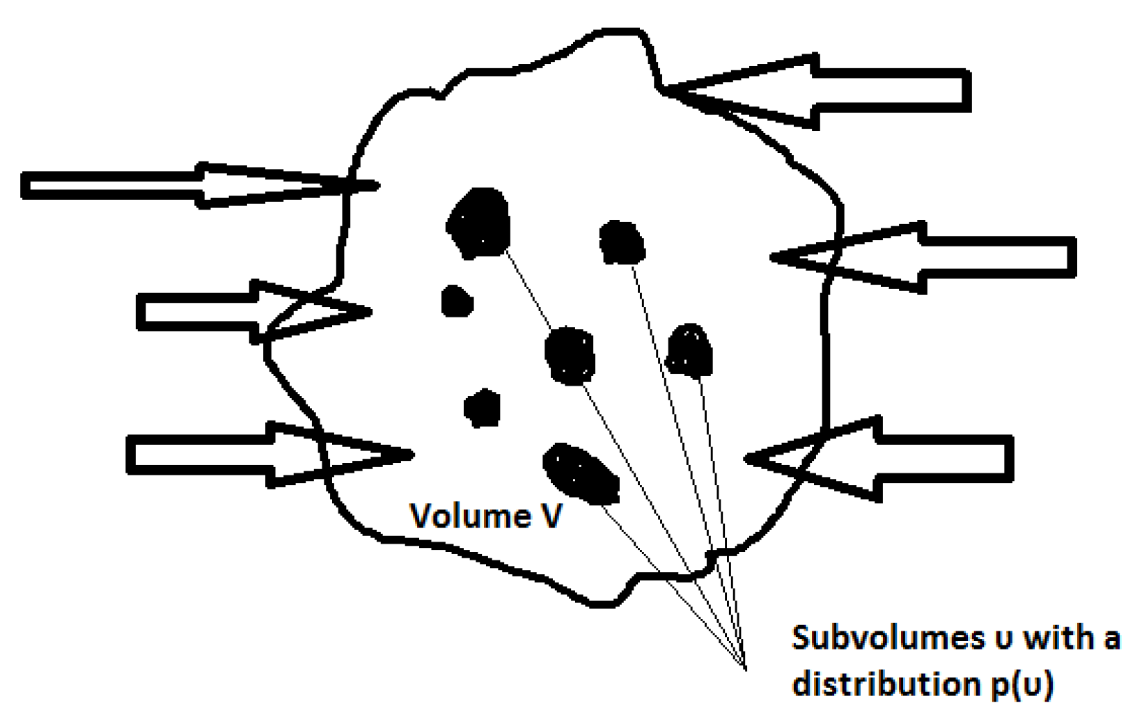
In the first initial phase the temporal and spatial distribution of seismic activity within
V is approximately uniform. During the initial phase the flow of tectonic elastic energy into
V is released with weak earthquakes and possibly with an additional aseismic deformation (e.g., creep). It is straightforward to accept that due to the inhomogeneity of the crust the elastic energy is concentrated in some subvolumes υ within
V (see
Figure 1). The latter leads to the increase of stress in subvolumes and at a critical time the configuration of the stress field specifies the parameters of the future main shock. To express the energy which supports stress we define as
the elastic energy surface density which tectonically flows within
V as
where
A is the area associated with the external bound of the volume
V. Τhe energy is released as seismic activity and we define
as the volume density of the elastic energy seismically released as a result of the earthquake activity within
. We note that
is formed by the set of all the earthquake subvolumes υ within
V,
), while an aseismic term
exists to describe the part of the inflow energy to
V which is not related to the earthquake activity.
According to the fundamental principle of energy conservation we have:
or:
where
assumed. Motivated from the Voight relation [
64], we generalized in Equation (3) the assumption suggested in [
16] (for
ξ = 1/2), accepting its validity for the generalized Benioff strain
Equation (3) relates the rate of the generalized Benioff deformation with the volume density of the elastic energy released and it is similar with that used in damage mechanics, where the evolution of the damage variable is related with the square of the strain [
65,
66,
67]. If
L is the characteristic size of the volume
V then
and
V where
de is the Euclidean dimension of
V which is
de = 3 when the earthquake activity in embedded in a 3 dimensional space and
de = 2 when it is located in an almost 2-dimensional surface. We clarify that hereafter the term “volume” has to be viewed as the geometrical size related with the spatial distribution of earthquake events and as mentioned it is the geometrical volume in the case of a 3-dimensional distribution of preshocks.
2.2. A Non Extensive Statistical Physics View of Generalized Benioff Deformation
We proceed now to the estimation of the probability distribution
p(υ) of the sub-volumes
υ that form the
Veff. To this direction, we introduce the principles of non-extensive statistical mechanics in our analysis. Its cornerstone which is recapitulated here, is the non-additive entropy
Sq [
34,
35], which is non-additive in the sense that it is not proportional to the number of the system’s elements, as in the Boltzmann-Gibbs entropy
SBG. The Tsallis entropy
Sq reads as:
or in equivalent form as
for a continuum variable
x, with
the definition of the q-logarithmic function and
kB is Boltzmann’s constant;
pi and
p(x) are the probabilities of
x;
W is the total number of microscopic configurations; and
q the entropic index. This last index is a measure of the non-additivity of the system and for the particular case
q = 1, the Boltzmann-Gibbs entropy
SBG is obtained;
. We note that for
q = 1, we obtain the well-known exponential distribution [
34]. The cases
q > 1 and
q < 1 correspond to sub-additivity and super-additivity, respectively. Although Tsallis entropy shares a lot of common properties with the Boltzmann-Gibbs entropy,
SBG is additive, whereas
Sq (
q ≠ 1) is non-additive [
34]. According to this property,
SBG exhibits only short-range correlations, and the total entropy depends on the size of the systems’ elements. Alternatively,
Sq allows all-length scale correlations and seems more adequate for complex dynamical systems, especially when long-range correlations between the elements of the system are present.
For a system composed of two statistically independent subsystems,
Σ1 and
Σ2, the Tsallis entropy satisfies the equation [
34]:
The non-additivity is indicated by the last term on the right side of the equation above and represents the interaction between the two subsystems
and
. In order to estimate the probability distribution
p(υ) of the seismic subvolume
υ, we maximized the non-extensive entropy under the appropriate constraints, using the Lagrange-multipliers method with the Lagrangian [
34,
35]:
The first constraint used refers to the normalization condition that reads as:
. Introducing the generalized expectation value (
q-expectation value),
υq which is defined as:
, where the escort probability is given in [
35] as:
, the extremization of
Sq with the above constraints yields to the probability distribution of
p(
υ) as [
68,
69]:
where
is a normalization coefficient. We recall that the
Q-exponential function is defined as:
The normalized cumulative number of seismic subvolumes
υ can be obtained by integrating the probability density function
p(υ) as:
where
N(>
υ) is the number of events with seismic volume larger than
υ. In the latter expression, if we define
, this leads to:
having a typical
Q-exponential form.
In the frame of non extensive statistical mechanics approach for earthquake volumes bigger than a given one
υo we find a power law description of the distribution function and in such a case the cumulative distribution is
with an exponent
. To have an estimate of
υο we select the volume where the power law approximation of
P(>υ) takes the value
P(>υ) = 1 leading to
. We observe that
β ≤ 1 leading to
, in agreement with previous published results on earth physics processes at a broad range of scales from laboratory up to geodynamic one [
70,
71]. It is obvious that the volume distribution
p(υ) could lead to an estimation of
Veff as
which for large volumes (i.e., moderate to significant events) has an asymptotic behavior
. or
Veff~
where
which generalizes and justify the expression introduced in [
16]. The latter expression implies that when
d > 0 (
q > 3/2),
presents a fractal distribution of earthquake volumes with a fractal dimension
, leading to
. The latter expression suggests that within NESP approach the entropic parameter
q is bounded by the Euclidean dimension
of the dmed system. When
then
, while for
we constrain
q in the range
.
After introducing Equation (2a) into Equation (3), the generalized Benioff stress rate could be expressed as follows:
When the time
t approaches the time to failure
and since
following [
16] an expansion of
(
t) when
is:
From Equation (6) it is obvious that
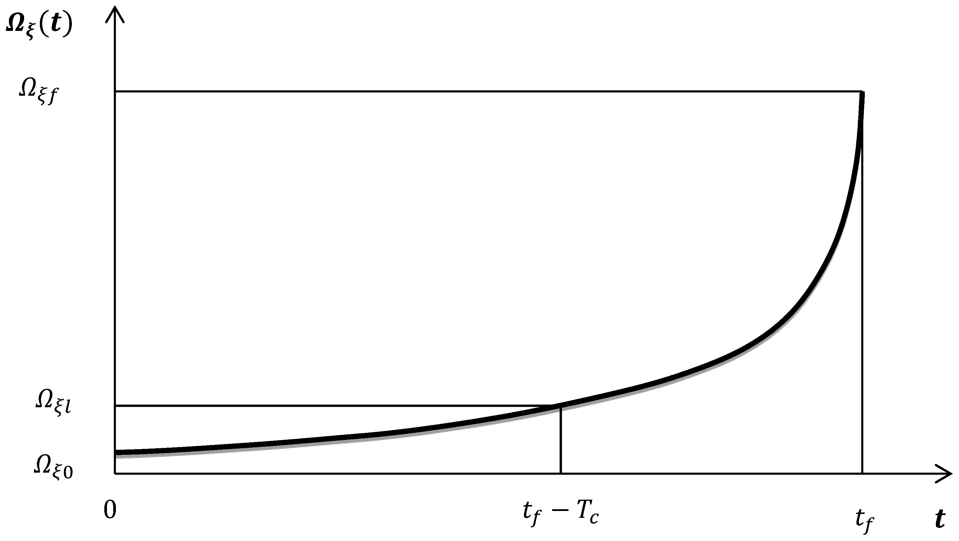
, expressing the elastic energy of tectonic origin inserted into the deformed area at the time of failure. The third term
. presents all the highest order terms in the expansion that are very small and could be omitted, while the parameter
is the characteristic time that defines the duration of the main shock preparation process starting from the time where deviation of
from linearity appears (see
Figure 2).
Approaching the main shock the volume where energy is released, defines a singular point [
16], and the analyticity assumption of
as
leads to:
A detailed discussion of Equation (7) is given in [
72,
73] where a scale invariance of the process is assumed in analogy with the theory of phase transitions. We note that when
,
and
. Substituting Equations (6) and (7) into (5) we obtain:
As
then
. Taking into account that
> 0 and
the first term in (8) dominates and the integration leads to:
which has the classical form proposed in [
4,
5,
6,
14] where:
The expression (10c) suggests that, is independent of ξ (0 ≤ ξ ≤ 1) introduced in the definition of the generalized Benioff strain but controlled by the Euclidean dimension . of the deformed system and the entropic parameter q which as a measure of long range interactions and of the complexity of the system, controls the distribution of seismic subvolumes υ and their fractality. It is worth to mention that the shape of the acceleration curve is controlled primarily by the exponent . Therefore, two differently sized main shocks with the same value will have similarly shaped acceleration curves but with different scale.
2.3. A NESP View of the ASR Parameters
The NESP approach could also be used to formulate the earthquake frequency-magnitude distribution [
44]. Moreover, [
44] introduced an energy distribution function that shows the influence of the size distribution of fragments on the energy distribution of earthquakes, including the Gutenberg—Richter (GR) law as a particular case. [
45] revised the fragment-asperity model using a more realistic relationship between earthquake energy (
E) and fragment size. Many recent works indicated that the
q parameter can be used as a measure of the stability of an active tectonic area [
40,
41,
44,
45,
70,
74]. A significant increase of
q indicates strong interactions between the fault blocks (earthquake volumes) and implies a transition away from equilibrium [
36,
37,
70]. Here we will modify the above mentioned models in order to formulate a frequency-magnitude distribution, taking into account the earthquake volume distribution
p(υ) and introducing a scaling law between the released relative energy (
E) and the earthquake volume (
υ) as has been proposed in [
45] in agreement with the scaling relationship between seismic moment and rupture length. From Equation (4) the energy distribution function of the earthquakes can be written as follows:
Since the probability of the energy is
, where
corresponds to the number of earthquakes with energy
and
is the total number of earthquakes, the normalized cumulative number of earthquakes is given as:
where
is the number of earthquakes with energy greater than
E. Combining Equations (11) and (12) the following expression for the earthquake frequency-energy distribution
is derived:
which for
suggests a scaling law
in agreement with the well known power law scaling
with
[
36,
37,
70,
75]. As proposed in [
76] the earthquake magnitude
M and the released seismic energy
E, are related as
, leading to a
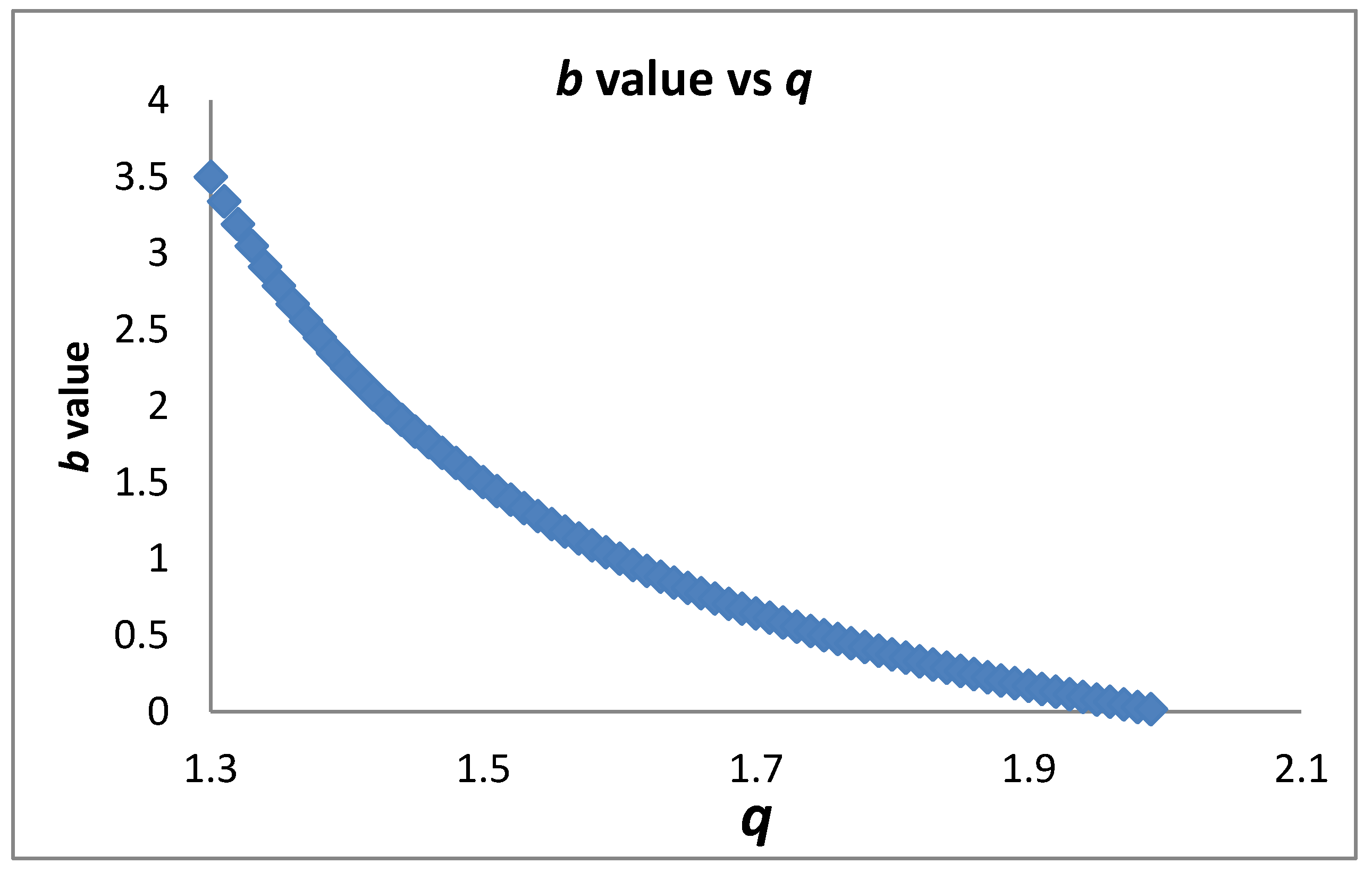
b-value in the Gutenberg—Richter law:
Figure 3 presents the dependence of the
b value on
q as given in (14). Substituting
into
as given by Equation (10c) and taking into account (14) we find:
which connects the non-extensive parameter
q and the
b-value of the Gutemberg—Richter law with the
parameter of the generalized Benioff strain. We note that in [
6] using synthetic data a relationship between
b-value and
was claimed. For the parameter
a positive definition is required (
and thus
. Theoretical results and experimental observation [
3,
4,
5,
6,
10,
11,
12,
13,
14,
15,
16,
17,
18,
19,
20,
21,
22,
23,
24,
25] suggest that
and
, while
should be the same for different
values, in agreement with observations that indicate
[
75]. Substituting
or
to (10c) we find
. From here on we will keep a constant value
in agreement with damage mechanics models where the evolution of the damage variable is related with the square of the strain [
65,
66,
67].
Equation (15) along with the constrain
leads to a lower bound for the
b value and an upper bound for the
q value, respectively, given as:
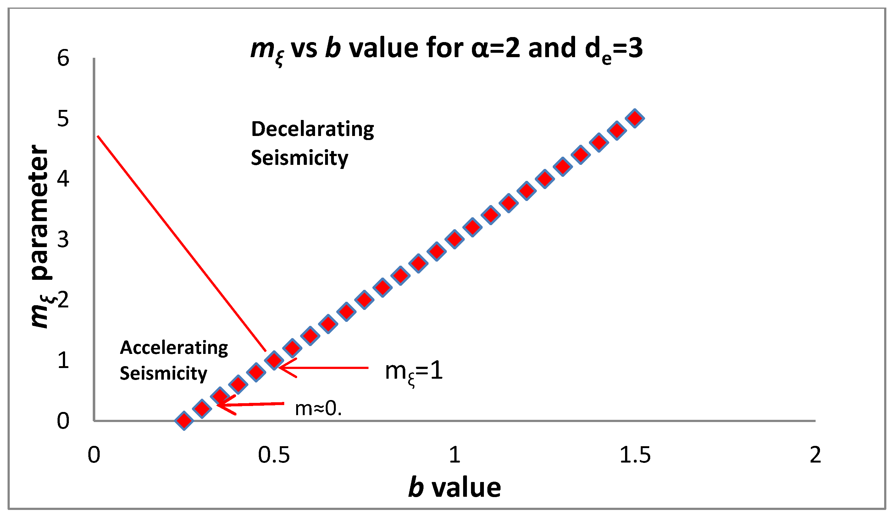
which for α = 2 and
while for
The maximum permitted value of
q is
qmax= 13/7 for
qmax = 9/5 for
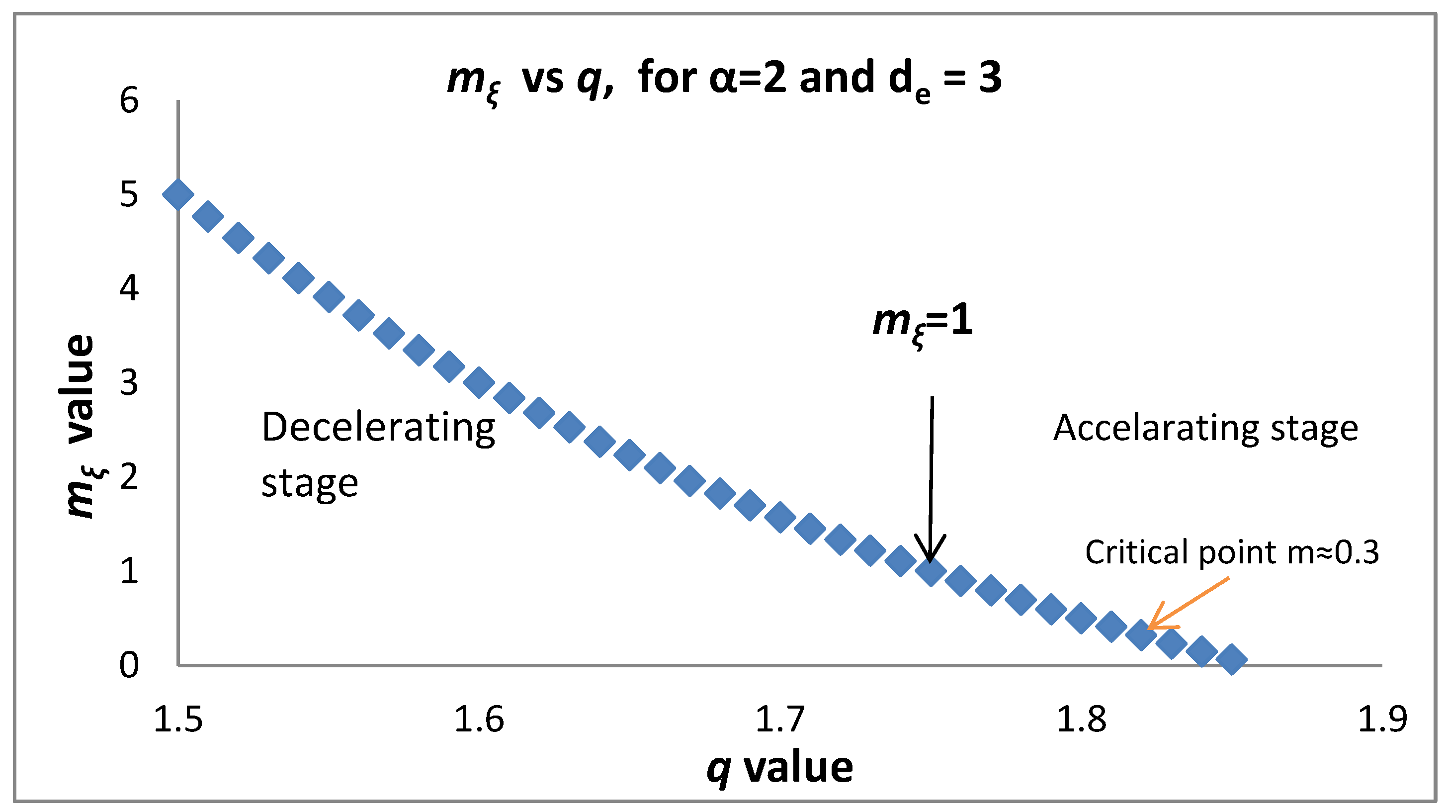
. For accelerating (decelerating) seismicity
(
). Applying Equation (15) shows that in accelerating seismicity
which implies a lower bound of the observed q introduced by the topological Euclidean dimension
of the space where the earthquakes are embedded. For
while for
. In a similar way we have
for decelerating seismicity. Furthermore, Equation (15) for
(accelerating seismicity) leads to
which (as we approach failure) for
leads to
and for
. The above expressions introduce a critical value for
q and for
b where a transition from decelerating to accelerating seismicity occurs. It is obvious that the decelerating seismicity which is described by
for
leads to
and for
.
Figure 4 and
Figure 5 present the dependence of
mξ on
q and
b, respectively.
Furthermore the above analysis could be applied to connect changes of
mξ to
b-value variations which have been reported as precursory effects in a number of significant earthquake events [
76,
77,
78,
79]. Equation (15) suggests that variations of the
b value are associated with the temporal evolution of
mξ during the main event preparation period
Tc, following the
b values changes as suggested in [
80]. We write
b(t) =
bo +
Λ(t) where
bo represents the background
b-value and
Λ(t) reflects the time dependent part of
b-value that varies during the preparation of the main earthquake event (see
Figure 6). Substituting in (15) we find:
For α = 2,
bo = 1 and
while for
,
, both describing a decelerating stage of seismicity. As we approach the failure time
tf, observational results suggest that
, leading to
for
and
for
, respectively.
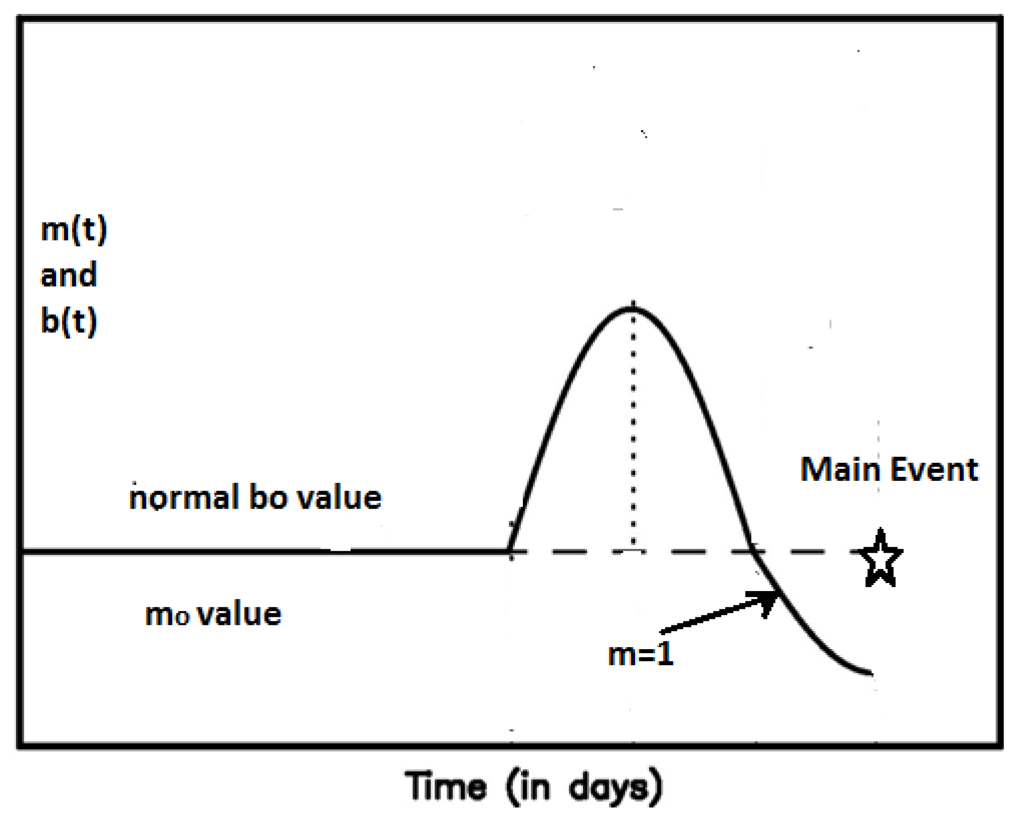
Figure 6 exhibits the general pattern of the temporal variation of the
mξ parameter following the temporal variation of the
b-value as suggested in [
80]. Most of the time after the last main event the
mξ value varies around
mξo, which corresponds to the average
bo value measured over a long time period. As the
b value increases from
bo to a maximum value (thus a seismic quiescense appears in agreement with [
24]), the parameter
mξ(t) increases too in a way following Equation (15). After passing a maximum value
mξmax, a decreasing phase of both
b and
mξ starts, crossing the value
mξο and approaching the transition time
tc where
mξ(tc) = 1, which defines the passing from the decelerating to an accelerating stage. At the next step
mξ(t) is approaching the value
which lies in the range of 0.25–0.35 and suggests the approach to a final stage of the preparation of the mainshock. The latter is in agreement with [
81,
82] where
b values based on seismicity over a period from 2006 till immediately before the Tohoku earthquake, revealed a zone of low
b value (
b ≈ 0.5–0.6) in and around the focal area as an indicator of highly stressed patches in the zone, in remarkable similarity to
b values obtained in laboratory experiments [
83]. We note that for
b ≈ 0.5 Equation (15) gives
m1/2 ≈ 0.3 in agreement with the value
m = 0.24 ± 0.09 given in [
84].
2.4. Fundamental Properties of the Function
Here we study some fundamental properties of the
function that could be used to understand the physics of many empirical laws presented in [
11,
15,
17,
19,
21]. From Equation (10b) we find:
The energy of the main shock is
or
. Experimental results and theoretical estimations suggest that the preparation time has a very weak dependence of the magnitude of the main shock. Substituting to Equation (17) the scaling laws
, we find
. Since
we conclude that the scaling factor has a value
, remarkably close to that observed in a number of works [
11,
15,
17,
19,
21].
From Equation (9) we calculate the generalized Benioff strain rate
:
According to Equations (9) and (18) we have:
and:
When
i.e., in the start of the accelerating deformation stage, we have:
It is physically reasonable to expect a continuity of physical parameters in the transition from the linear to the accelerating deformation period and to accept that at
a continuity of the generalized Benioff strain rate gives:
where
is the slope of the linear part. We calculate the mean generalized Benioff rate during the accelerated (deformed) period
i.e., from
to
:
From (20) and (21) we reach the conclusion that:
Furthermore from (19), if
we have:
. Combining the latter expression for
with Equation (21) leads to:
which is exactly the expression proposed in [
11,
15,
17,
19,
21]. Equation (22) could be written as:
which indicates that if we estimate
and the slope of the linear part of the generalized Benioff strain we can estimate at least the order of magnitude of
at the time of failure.
Let us assume that the last earthquake prior the main shock appears at a time
. Applying the time to failure Equation (9) we have:
or:
Even if our approach is general, from here on, we limit ourselves to the case
ξ = 1/2 describing the Benioff strain which is very commonly applied. In this case the Benioff stain of the main shock is:
resulting in:
Since the seismic energy is related to seismic magnitude by the relation:
Using previously published observational estimates [
11,
15,
17,
19,
21] for
ξ = 1/2 we have an order of magnitude estimation for the parameter
, and assuming
with
and the last main preshock to appear at:
(i.e.,
), the expected earthquake magnitude of the main event should be of the order of
. In addition, since
from Equation (24) we have the constraint
, which leads to the conclusion that the maximum expected earthquake magnitude in an area with background Benioff strain rate
is:
It is obvious that the ratio
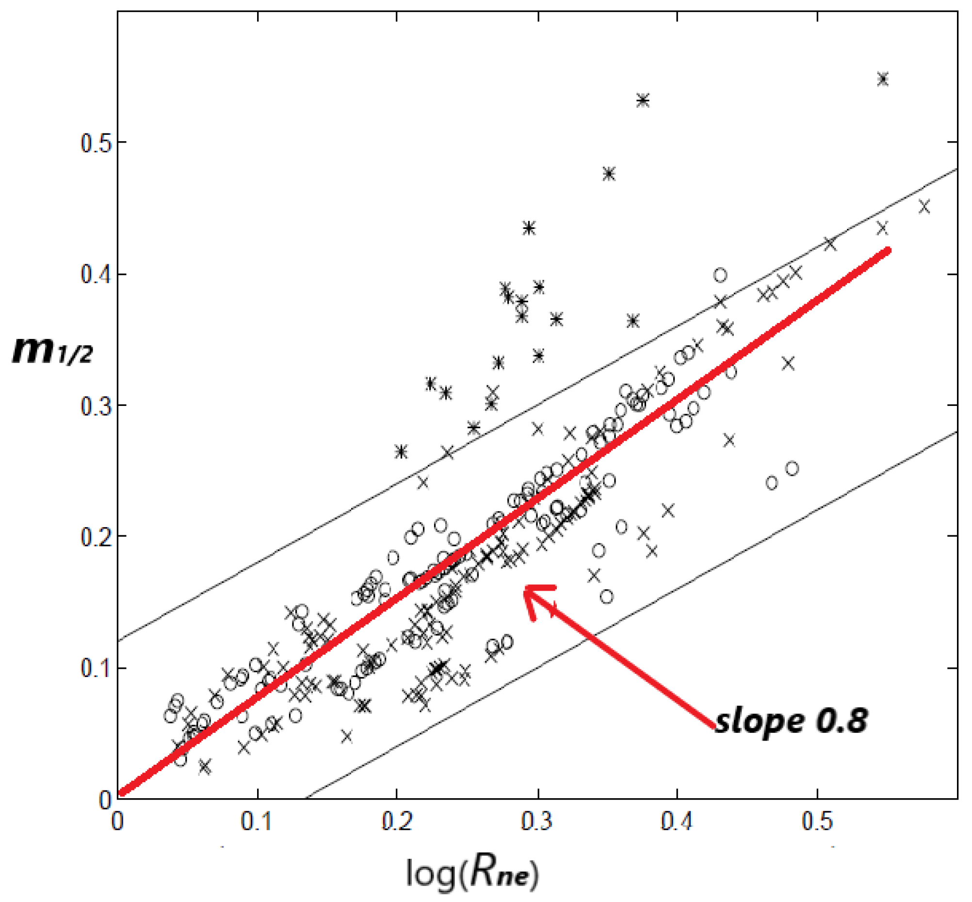
is a crucial parameter to define the final stage of the main event preparation. [
10] proposed a relationship between
and the normalized energy released
Rne which is defined as the total cumulative square root energy (i.e.,
ξ = 1/2) divided by the square root of the energy released by the main shock. Thus
. From the previous expressions it is obtained that
which leads to:
in which a linear relation between
m-parameter and
is suggested with a positive slope
since
Tc >
δt1). The
Figure 7 from [
10] is reproduced here (as
Figure 7) and a red line with a slope of the order of 0.8–1.0 is added to the figure that seems to describe the majority of the data points. The latter slope permits an order of magnitude estimation of the ratio
, leading to
.
3. Concluding Remarks
The organization patterns that earthquakes and faults exhibit has motivated the statistical physics approach to earthquake occurrence [
85]. Based on non-extensive statistical physics and the Tsallis entropy a framework that produces the collective pattern of seismicity has been introduced to describe the macroscopic behavior of complex seismic systems that present strong correlations among their elements [
70]. Observational indications support the hypothesis that many large earthquakes are preceded by accelerating-decelerating seismic release rates which are described by a power law time to failure relation. The question whether accelerating/decelerating seismicity is described in terms of non-extensive statistical physics presents a challenge. This is the problem addressed in the present work. Motivated by a simple model originally proposed in [
16] where fundamental concepts such as that of energy conservation are used to understand the accelerating seismicity we generalized it by introducing the concept of generalized Benioff strain which is merged with ideas of complexity and non-extensive statistical physics.
In the present work, a unified theoretical framework is discussed based on the ideas of non-extensive statistical physics along with fundamental principles of physics such as the energy conservation in a faulted crustal volume undergoing tectonic stress loading. We define a generalized Benioff strain function where and a time-to-failure power-law of derived using the fundamental principle of energy conservation in a fault system that obeys a hierarchical distribution law extracted from Tsallis entropy. In the time-to-failure power-law that follows the existence of a common exponent mξ which is a function of the non-extensive entropic parameter q is demonstrated.
Since
, with
B =
and:
the properties of these parameters have been studied and their upper and lower bound of the parameters
q and
b created according the geometrical limitations, the positive definition of
mξ and the condition of the system (accelerating with
mξ < 1 or decelerating with
mξ > 1). The range of
q and
b values that could drive the system into an accelerating stage and to failure has been discussed, along with the precursory variations of
mξ as resulting from the appearance of precursory
b-value anomaly.
It has been proved that . where is the mean generalized Benioff sain rate during the accelerated (deformed) period , while where refers tthe generalized Benioff strain rate during the linear stationary part of . A discussion of a number of empirical scaling laws is given, among them the scaling of B with the magnitude of the main even produced from first principles in agreement with the empirical one.
Our calculations based on Tsallis entropy and the energy conservation give a new view on the empirical laws presented in the literature, the associated average generalized Benioff strain rate during the accelerating period with the background rate and connected model parameters with the expected magnitude of the main shock. The need for accurate earthquake catalogues that will support (or not) further theoretical results which are still in debate [
86], is stressed.


