Article

GYMEE: A Global Field-Scale Crop Yield and ET Mapper in Google Earth Engine Based on Landsat, Weather, and Soil Data

Department of Agriculture, Faculty of Agricultural and Food Sciences, American University of Beirut, Beirut 2020-1100, Lebanon
*
Author to whom correspondence should be addressed.
Remote Sens. 2021, 13(4), 773; https://doi.org/10.3390/rs13040773
Submission received: 12 January 2021 / Revised: 3 February 2021 / Accepted: 4 February 2021 / Published: 20 February 2021

Abstract

:
In this study, we used Landsat Earth observations and gridded weather data along with global soil datasets available in Google Earth Engine (GEE) to estimate crop yield at 30 m resolution. We implemented a remote sensing and evapotranspiration-based light use efficiency model globally and integrated abiotic environmental stressors (temperature, soil moisture, and vapor deficit stressors). The operational model (Global Yield Mapper in Earth Engine (GYMEE)) was validated against actual yield data for three agricultural schemes with different climatic, soil, and management conditions located in Lebanon, Brazil, and Spain. Field-level crop yield data on wheat, potato, and corn for 2015–2020 were used for assessment. The performance of GYMEE was statistically evaluated through root-mean-square error (RMSE), mean absolute error (MAE), mean bias error (MBE), relative error (RE), and index of agreement (d). The results showed that the absolute difference between the modeled and predicted field-level yield was within ±16% for the analyzed crops in both Brazil and Lebanon study sites and within ±15% in the Spain site (except for two fields). GYMEE performed best for wheat crop in Lebanon with a low RMSE (0.6 t/ha), MAE (0.5 t/ha), MBE (−0.06 t/ha), and RE (0.83%). A very good agreement was observed for all analyzed crop yields, with an index of agreement (d) averaging at 0.8 in all studied sites. GYMEE shows potential in providing yield estimates for potato, wheat, and corn yields at a relative error of ±6%. We also quantified and spatialized the soil moisture stress constraint and its impact on reducing biomass production. A showcasing of moisture stress impact on two emphasized fields from the Lebanon site revealed that a 12% difference in soil moisture stress can decrease yield by 17%. A comparison between the 2017 and 2018 seasons for the potato culture of Lebanon showed that the 2017 season with lower abiotic stresses had higher light use efficiency, above-ground biomass, and yield by 5%, 10%, and 9%, respectively. The results show that the model is of high value for assessing global food production.

Graphical Abstract

1. Introduction

Crop yield modeling and prediction have broad implications on global food security and food production monitoring. Decision makers depend on yield information to determine the potential reduction in crop yield, to deliberate food prices, and to make timely import and export decisions [1]. Farmers can benefit from crop yield modeling tools to monitor crop development throughout the growing season [2] and assess the need for fertilizer applications [3], irrigation [4], and disease control [5]. Many yield forecast approaches have been discussed in the literature, and each has its advantages and limitations. Examples are farmers’ reports [6], crop simulation models [7], remote sensing [8], and, recently, artificial intelligence techniques [9]. Crop yield prediction has long been founded on conventional methods, where ground-based crop and yield data are collected from field reports [10]. Nevertheless, this method is costly, and the data collected are not open access. This method is limited in scale, and it can have significant sources of errors as farmers may overestimate their yields. The collected yield data might be available too late for appropriate actions in some countries [6]. Crop models have been developed to overcome the limitations of the technique [11]. The crop models estimate crop yield based on daily crop growth simulators for a wide range of environments under the condition that the input data are accurate and sufficient [12]. Crop models can be based on either light use efficiency (LUE) or water use efficiency (WUE). Both variables are hard to estimate with certainty because they rely on many other parameters that are difficult to measure on a large scale. The LUE approach relies on the efficiency of the crop to convert the light absorbed or the water transpired into biomass [13,14]. The fraction of the absorbed photosynthetic active radiation (FPAR) is used as a key parameter for these models such as crop-environment resource synthesis (CERES) [15], Environmental Policy Integrated Climate (EPIC) [16], and Decision Support System for Agro-technology Transfer (DSSAT) [17]. The WUE approach relies on estimating the crop transpiration as a key parameter for crop yield modeling. Examples of such models are AquaCrop [18] and CropSyst [19].
Although crop yield models can be applied on different scales ranging from a point on a field to a region, they inherit some limitations [11,20]. The difficulty lies in characterizing the large spatial variability across crops, soils, water, nutrient applications, stress factors, and initial system conditions, which hinder the use of several crop yield models. An additional limitation is the need for the local calibration of these models. To improve yield prediction, numerous approaches based on the assimilation of satellite observations into the crop models have been used. The integration of the remotely sensed leaf area index (LAI) has increased the performance of growth models [21,22,23]. The advantage of this approach is that the LAI partially reduces the need to characterize the crop growth conditions, but not the need for model calibration and determination of the initial system conditions, as reported by Khan [11]. Other approaches rely on correlating the modeled yield with vegetation spectral indices (VIs) derived from satellite images [24]. The major drawback of using this method is that this correlation exhibits an empirical character and that the correlation coefficient is usually moderate to low [25,26].
Many researchers suggest that the radiation or light use efficiency (LUE)-based biomass model proposed by Monteith [27] has significant potential for estimating the crop yield when combined with satellite data [28,29]. The LUE model was implemented using medium-resolution sensors like Moderate Resolution Imaging Spectroradiometer (MODIS) [30,31] and Advanced Very-High-Resolution Radiometer(AVHRR) [32] to monitor biomass production over a regional scale at high temporal resolution. However, the disadvantage of the application of medium-resolution data is that they cannot be applied to small fields due to large pixels. Pan et al. [33] applied the LUE model using higher data like Landsat but relied on a few images. Campos et al. [34] used the water productivity model to estimate crop yield and suggested considering the effect of the incoming radiation as a limitation for biomass production of wheat fields but without considering the environmental stresses.
In the present work, we developed the backend of a Google Earth Engine (GEE)-based operational model to estimate the global crop yield at 30 m resolution based on remote sensing. The Global Yield and Evaporation Mapper in Earth Engine (GYMEE) was validated herein in three countries, Lebanon, Brazil, and Spain, during 2015–2020. GYMEE was used to model yields of potato (Solanum tuberosum), wheat (Triticum aestivum) in Bekaa Valley (Lebanon), corn (Zea mays L.) in São Desidério, Brazil, and wheat (T. aestivum) in Albacete, Spain. The analyzed crops are of strategic importance in the study sites, and the availability of field-level, ground-based yield data for these crops presents an opportunity to test our estimates. Wheat culture is one of the most dominant in the Mediterranean region (Lebanon and Spain). The analyzed wheat fields from the southeast of Spain cover an extensive range of average yields (1.2–10.3 t/ha). The range of obtained wheat yield in Spain represents the maximum and minimum wheat production in the area. On the other hand, the wheat culture in Lebanon is commonly planted in West Bekaa on farms between 0.2 and 300 ha in size [35]. Both west and center Bekaa have the highest production of wheat (44% of the national total). The average wheat yield reported in 2019 was 4.58 t/ha [35], ranging between 1 t/ha (for rain-fed) and 8 t/ha (with supplementary irrigation). Potato is considered a major cash crop in Bekaa Valley, where more than 19,000 ha are planted every year [36,37]. The potato yield in Bekaa varies between 20 and 50 t/ha, with an average of 23 t/ha [38]. Additionally, Lebanon produces around 400,000 tons of potato [38], more than two-thirds of which is grown in the Bekaa plain. Corn is considered the third-most valuable crop in the western region of the state of Bahia, Brazil, conquering an area corresponding to 180,000ha in 2016–2017, with a total production of 1,404,000tons and an average yield of 7.8t/ha [39]. The primary objectives of this analysis were to (1) assess the validity of integrating remotely sensed energy balance evapotranspiration modeling with the derived, modified Monteith model in obtaining crop yield, (2) evaluate the potential application of the operational model under different climatic and management conditions, (3) analyze the temporal and spatial variations in above-ground biomass and yield, and (4) investigate the effect of the inclusion of environmental stresses (vapor, temperature, and moisture) on the crop yield modeling process through showcasing examples from the study sites.

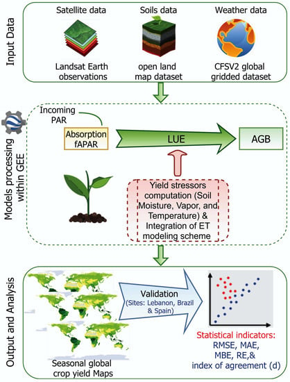
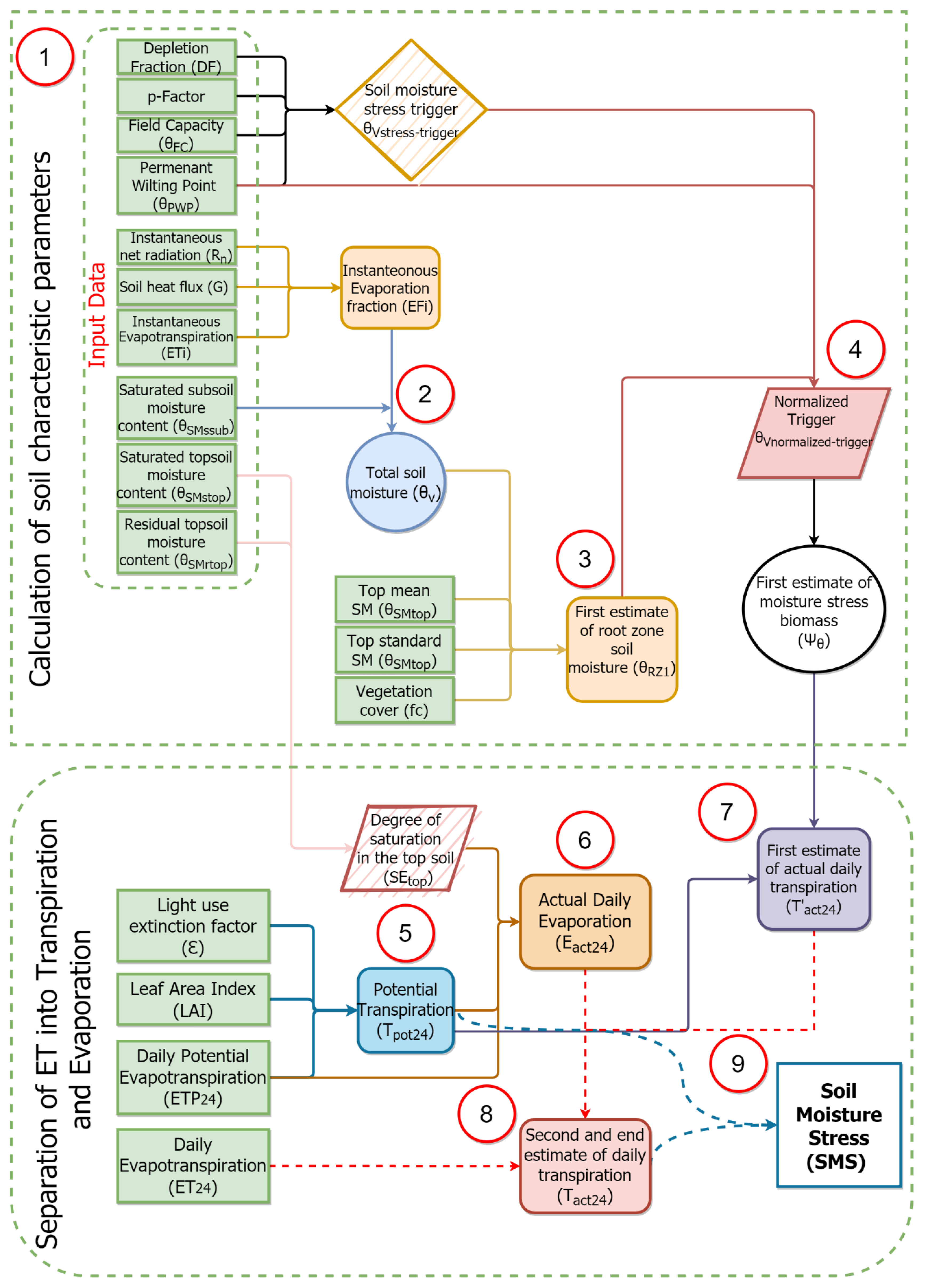
2. Basis of the Model for Above-Ground Biomass (AGB) and Crop Yield Estimation

The above-ground biomass (AGB) is calculated as a product of the absorbed photosynthetic active radiation (APAR, MJ/m2/day) [27] and light use efficiency (LUE) [40]. The model considers the impact of the environmental conditions affecting biomass production, notably for the impact of temperature stress (TS), vapor stress (VS), and soil moisture stress (SMS). The relationship between the factors is given as:
AGB = APAR × LUE max × TS × VS × SMS × 0.864
where AGB (kg/ha) is the dry above-ground biomass production for the day of the satellite overpass; APAR is the absorbed photon flux by the canopy photosynthetic elements; LUE max is the maximum light use efficiency (g/MJ); TS, VS, and SMS are the temperature, vapor, and soil moisture stressors, respectively; and 0.864 is a unit conversion factor [41]. The actual LUE (LUEmax multiplied by the stresses) is a relatively constant property of the crop, with a distinction between C3 and C4 crops [27]. There are several studies on the determination of the LUEmax for crops, varying between 1.44 and 3.22 for C3 crops [42,43,44,45] and between 3.27 and 4.26 for C4 crops [46,47]. Still, there is no consensus in the scientific community on the LUEmax for crops. An annual global crop map is still not available. Here, we use a constant value of LUEmax (2.5 for C3 crops—wheat and potato) and 3.5 for C4 crops (corn) [32]. Values of LUEmax can be linked to a global crop map as it becomes available in GEE. The stress factors are expressed as fractions, with 0 indicating extreme stress and 1 indicating no stress. Details on the estimation of APAR and the stresses are provided in Section 2.1 and Section 2.2.
To derive crop yields, the mean dry biomass production for each field at each date of the satellite overpass needs to be accumulated over the growing season of each crop by interpolating between satellite imagery dates to fill in the missing dates. The accumulated biomass is converted into yield through crop harvest indices and the percentage moisture content of the crop at harvest [48]. Crop yield (t/ha) is calculated as:
EY i = AGDB i × HI i 1 % Moisture
where EYi is referred to as the metric tons of economic yield per hectare of crop i, AGDB is the accumulated above-ground dry biomass, and HIi is the harvest index of crop i, which is the ratio of yield to above-ground biomass.

2.1. Remote Sensing of Active Photosynthetic Radiation (APAR)

APAR is approximated directly from photosynthetic active radiation (PAR) and fraction of photosynthetic active radiation (fPAR; intercepted by the leaves and used in the carbon dioxide assimilation process).
APAR = fPAR × PAR daily
The link between fPAR and LAI and the normalized difference vegetation index (NDVI) have been thoroughly documented in the literature as useful indicators of crop growth in yield models [49,50]. fPAR can be calculated using the NDVI [51,52] as:
fPAR = { 0.161 + 1.257 × NDVI for   NDVI 0.125 0 Otherwise
where an NDVI value of 0.125 indicates bare soil [52].
The photosynthetic active radiation (PAR, MJ/m2/day) represents the spectral range from 400 to 700 nm used by the canopy’s photosynthetic elements [53]. PAR is a fraction of the incident shortwave solar radiation (Rs) [54]. Rs can be obtained from climatic data (National Oceanic and Atmospheric Administration’s (NOAA) climate forecast CFSv2 or Copernicus ECMWF models, both of which are available in GEE), or it can be estimated as a function of daily extraterrestrial radiation R a and atmospheric transmissivity τ w as follows (our choice):
PAR daily = 0.48 × R a × τ w
where atmospheric transmissivity can be calculated from water vapor and extraterrestrial solar radiation ( R a ) can be calculated from the solar constant, solar declination, and day of the year [55].

2.2. Calculations of Yield Stressors

2.2.1. Vapor Stress (VS)

The vapor stress factor shows how evapotranspiration and photosynthetic processes are affected by vapor pressure [56]. The VS is estimated from a link with the vapor pressure deficit (VPD) (for relative humidity less than 100%) [57,58]. The VPD is defined as the difference between the saturated and the actual vapor pressure. It is considered a critical driver of the water and carbon demand for crops [59], where increases in the VPD can reduce the uptake of carbon and water use by the plant [60].
VS = 0.88 0.183 × log ( e s e a )
where es and ea are the saturated vapor pressure and the actual vapor pressure (KPa), respectively.

2.2.2. Plant Temperature Constraint (TS)

The temperature stress (TS) was used according to Stewart [61] and Stewart [62]. The author proposed a relationship between the TS and the Jarvis coefficient (Jc) after Jarvis [63]. The TS is computed as a function of the daily temperature, upper and lower limit stomatal activity, and optimum conductance temperature of the crop.
TS = ( T T L ) × ( T H T ) J c ( K T T L ) × ( T H K T ) J c
where Jc is the Jarvis coefficient calculated according to Equation (8).
J c = T H K T K T T L
where T is the air temperature (°C), TH is the upper limit of stomatal activity set equal to 45 (°C), KT is the optimum conductance temperature (°C) set equal to 24, and TL is the lower limit of stomatal activity. It is set equal to 0 °C [64]. For mean daily air temperatures higher than 40 °C, the TS is set to 0.001. Values of TH, KT, and TL are obtained from Maidment [65].

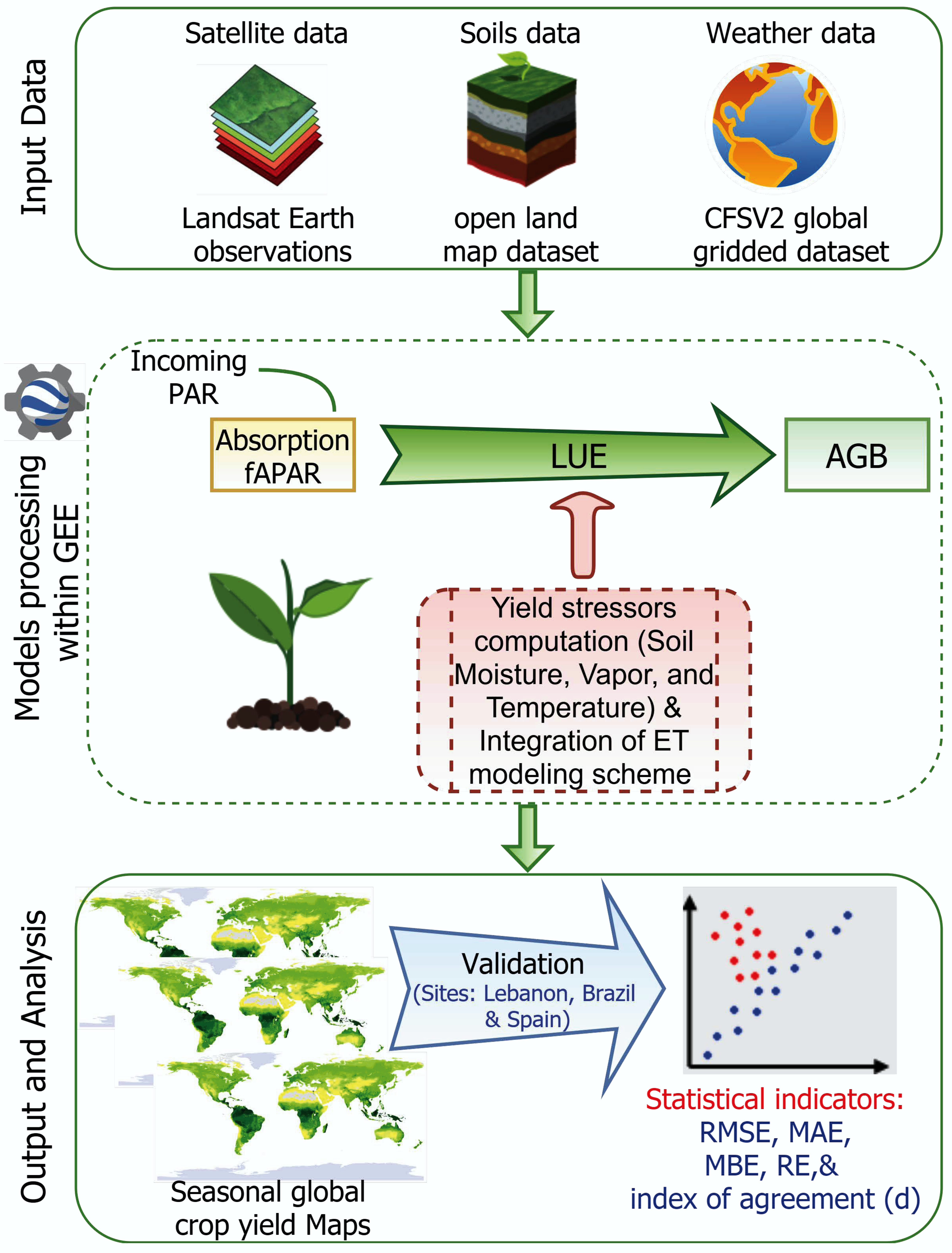
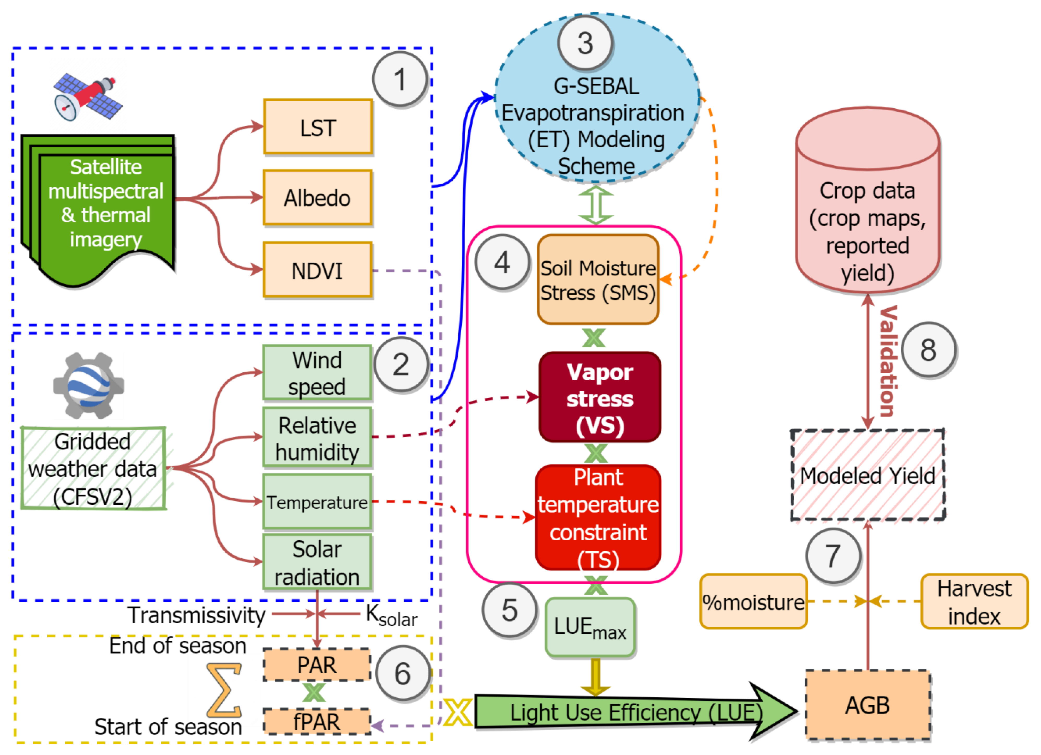
2.2.3. Soil Moisture Stress (SMS)

Surface energy balance retrieval of evapotranspiration (ET) has been used as an indicator of soil moisture availability and vegetation health [66,67,68]. In this study, we use the soil moisture stress factor as an indicator of agricultural drought. The SMS describes anomalies in the actual-to-potential 24 h transpiration ratio (Tact24/Tpot24) [69] via the energy balance. An overview of the step-by-step procedure for calculating the SMS is given in Figure 1.

2.2.4. Daily Actual ET Modeling Scheme

The energy balance scheme incorporates key meteorological variables proven to provide early warning of declining crop moisture conditions [70,71,72]. Many models can be utilized to estimate evapotranspiration (ET) as a residual of the energy balance, such as DisAlexi and Two-Source Energy Balance (TSEB) [70], Mapping Evapotranspiration at High Resolution with Internalized Calibration (METRIC) [73], Surface Energy Balance Algorithm for Land (SEBAL) [74], Surface Energy Balance (SEB), or Simplified Surface Energy Balance (SSEB) [75]. In this work, we estimated ET based on the latest version of the single-source Surface Energy Balance for Land (pySEBAL) model described thoroughly in Jaafar and Ahmad [76]. We coded pySEBAL in Google Earth Engine, and it can be applied globally to any Landsat 7 or 8 collection and to Sentinel-2–MODIS–VIIRS (Visible Infrared Imaging Radiometer Suite) combination. Briefly, pySEBAL is an improved and automated version of SEBAL [74]. We refer to the GEE version of pySEBAL we developed as G-SEBAL. G-SEBAL performs energy balance at the satellite (Landsat 7 or 8 or Sentinel-2) overpass time to obtain the latent heat flux (λE, W.m−2) as the residual of the surface energy equation ( λ E = R n G H ) . Net radiation ( R n ) is composed of net shortwave radiation and net longwave radiation. The former depends on the surface albedo and solar irradiation, while the latter depends on emissivity and surface and air temperatures. R n is computed as an average of the Food and Agriculture Organization (FAO) equation [77] and the Slob equation [78]. The soil heat flux (G) is calculated from a semi-empirical approach as a function of the NDVI, surface temperature, and albedo [79]. The sensible heat flux (H) is computed via a single-source resistance scheme using an iterative process through relating the air density ( ρ a i r ), the specific heat of air at constant pressure ( C p ), and the near-surface temperature difference ( dT ) to aerodynamic resistance ( r a h ) [80]. dT is estimated as a linear function of the corrected surface temperature [79]. Aerodynamic resistance rah is calculated iteratively based on Monin–Obukhov similarity theory until a stable value is reached to calculate the near-surface temperature difference dT at the hot pixel where the ET is assumed to be zero. dT at the cold pixel is then calculated, and the relationship is used to derive dT and therefore H at all pixels in the image. We sharpen the surface temperature using a combination of a T-sHARP thermal sharpening approach and a bilinear moving window interpolation approach to identify an ensemble of hot and cold pixels automatically in GEE [81]. Afterward, we convert the instantaneous ET (derived from the instantaneous latent heat) to daily observations by utilizing the constant evaporative fraction (EF) assumption (EF = LE/[RnG]) [82], multiplied by an advection factor Ω [ Ω = 1 + 0.985 × EF × ( exp [ ( VPD ) × 0.08 ] 1.0 ) ] (a function of the vapor pressure deficit (VPD)) to account for the increase in the ET during the afternoon period [83]. Daily grass-reference evapotranspiration ETref is calculated from the Penman–Monteith evapotranspiration equation [65]. The potential ET ( ETP 24 ) is set equal to ET 24 if the latter is higher than ETref or to ETref otherwise. A digital elevation model (DEM) is used to calculate the slope, the aspect of terrain, and solar angles (latitude, declination, solar zenith angle, and solar incidence angle), to adjust land surface temperature (LST) and to correct ETref in the sloped terrains.

2.2.5. Soil Water Properties

To determine the soil moisture stress, it is essential to derive an estimate of soil moisture. Remote-sensing-based field-scale estimation of root zone soil moisture is still a challenging task. We utilize the Open Land Map Earth Engine dataset to derive soil texture and other properties. Field capacity, permanent wilting point, top, and subsoil saturated moisture content, and subsoil residual moisture content are all inferred from the soil physical properties. The soil texture and organic matter content are used to estimate the soil water properties, as explained in Saxton and Rawls [84], and the equations are coded in Google Earth Engine. We use the Open Land Map Earth Engine dataset [85] available in GEE to determine the soil texture of the different soil layers. The dataset uses a compilation of published point data coming from various national and international soil point-data providers, such as the FAOs soil profile databases, among many others for mapping soil properties and classes. The dataset is one of the products of OpenLandMap.org, which provides global gridded environmental layers based on ensemble machine learning. The soil data used herein are the organic carbon, clay, and sand content at six standard depths (0, 10, 30, 60, 100, and 200 cm) at 250 m spatial resolution. We then apply Saxton equations [84] to derive the potential water content at the field capacity and the permanent wilting point so as to calculate the plants’ available water in the top (0–60) and subsoil layers (60–100). We restrict the analysis to 1 m to account for areas where the bedrock is limiting.

2.2.6. Total Soil Moisture Content ( θ v )

We calculate the soil moisture content ( θ v ) as a function of the instantaneous evaporation fraction and the saturated soil moisture level in the subsoil (θSMssub) (see Equation (9)):
θ v = θ S M s s u b   × exp   ( EF i a b )
where a and b are curve-fitting parameters, 1 and 0.421, respectively [86]. The evaporative fraction describes the segregation of the net radiation into latent heat flux. It is intrinsically restrained by the soil moisture in the root zone [87].

2.2.7. A First Estimate of the Root Zone Soil Moisture ( θ V R Z 1 )

The root zone soil moisture’s first estimate ( θ V R Z 1 ) is calculated as a function of the fraction of vegetation cover (fc), with an initial assumption that the topsoil moisture as well as the root zone soil moisture ( θ V R Z ) is equal to the total soil moisture ( θ v ) [65]. The mean and the standard deviation of the topsoil moisture ( θ S M t o p m e a n and θ S M t o p s t d ), as well as the maximum and mean root zone soil moisture ( θ V R Z m a x and θ V R Z m e a n ), are computed from the total soil moisture (see Equation (10)). The first estimate of the root zone soil moisture is constrained between the residual subsoil moisture ( θ S M r s u b ) and the maximum moisture content M a x θ V R Z m a x (i.e., if the first estimate θ V R Z 1 is less than or equal to the residual subsoil moisture ( θ S M r s u b ), it is then set to the residual subsoil moisture, and if θ V R Z 1 is greater than or equal to M a x θ V R Z , it is set equal to M a x θ V R Z ).
θ V R Z 1 = θ V ( θ S M t o p m e a n + θ S M t o p s t d ) × ( 1 f c ) f c
M a x θ V R Z = f c × ( θ V R Z m a x θ V R Z m e a n ) + θ V R Z m e a n

2.2.8. Soil Moisture Stress Trigger ( θ V s t r e s s t r i g g e r ) and a First Estimate of Moisture Stress Biomass ( Ψ θ )

The soil moisture stress trigger ( θ V s t r e s s t r i g g e r ) is the critical value under which plants get stressed [88] computed as a function of the soil moisture at field capacity ( θ F C ) , soil moisture at permanent wilting point ( θ P W P ) , and the fraction of the total available water that can be depleted from the root zone before moisture stress (p-factor) [65]:
θ V s t r e s s t r i g g e r = θ F C p   factor × ( θ F C θ P W P )
p   factor = DF + 0.04 × ( 5.0 ET 24 )
where ET 24 is the daily actual evapotranspiration derived from the energy balance (Section 2.2.4) and DF is a crop-dependent depletion factor (a user-defined value). The depletion factor differs from one crop to another, and it usually varies from 0.30 for shallow-rooted plants at higher rates of crop evapotranspiration (>8 mm/d) to 0.70 for deep-rooted plants at lower rates of crop evapotranspiration (<3 mm/d). A value of 0.4 was used herein (potatoes are stressed at 0.3, while wheat and corn at 0.5). It is better, of course, to derive a map of the allowable depletion from crop maps, when available.
The first estimate of the root zone soil moisture (Section 2.2.7) along with the stress trigger (Equation (12)) are used to calculate the normalized stress trigger ( θ V n o r m a l i z e d t r i g g e r ) representing the effective fraction of available soil moisture [87] (Equation (14)). The first estimate of the moisture stress on the biomass ( Ψ θ ) is estimated as a function of θ V n o r m a l i z e d t r i g g e r (Equation (15)):
θ V n o r m a l i z e d t r i g g e r = θ R Z 1 θ P W P θ V s t r e s s t r i g g e r + 0.02 θ P W P
Ψ θ = { θ V n o r m a l i z e d t r i g g e r sin ( 2 π × θ V n o r m a l i z e d t r i g g e r ) 2 π 0.5 × FPAR for   Ψ θ < 0.5 × FPAR
where Ψθ is limited between 0 and 1.

2.2.9. Splitting the ET into Evaporation and Transpiration

To calculate the SMS factor, ETP 24 (Section 2.2.4) is split into its component of potential transpiration using an LAI-derived vegetation cover fraction light use extinction factor (ε) [89,90]:
T p o t 24 = ( 1 e ( ( ε × LAI ) ) ) × ETP 24
Alternatively, the LAI can be calculated from a remotely sensed estimate of fc derived from the NDVI [91,92]:
LAI = ln [ ( f c 1 ) ] 0.45
The LAI is restricted to the range of 0.001–8.
f c = 1 ( 0.8 NDVI 0.8 0.125 ) 0.7
where fc is set equal to 0 when the NDVI is less or equal to 0.125 (representing bare soil) and equivalent to 0.99 for an NDVI greater than 0.8.
Having calculated T p o t 24 , the actual evaporation (Eact24) component can be estimated using the topsoil saturation degree (SEtop) calculated from the topsoil water properties [93]. As presented in Equation (19), Eact2 is calculated from the difference between ETP24 and Tpot24 and either 1 or 1/(SEtop + 0.1)−2:
E a c t 24 = M i n ( 1 , 1 ( S E t o p + 0.1 ) 2 ) × ( ETP 24 T p o t 24 )
where SEtop is the degree of soil saturation of the topsoil, scaled between 0 and 1:
S E t o p = θ S M t o p θ S M r t o p θ S M s t o p θ S M r t o p
where θ S M t o p is the topsoil moisture and θ S M r t o p and θ S M s t o p are the residual and the saturated topsoil moisture, respectively, and are constants for a specific soil type.
The product of the first estimate of moisture stress biomass ( Ψ θ ) (Section 2.2.8) and T p o t 24 provides the first estimate of daily actual transpiration ( T a c t 24 ) [94]:
T a c t 24 = Ψ θ × T p o t 24
where T a c t 24 is set to zero when there is no vegetation cover.
The relative value of Tact24 and E a c t 24 are used to break down the ET 24 flux into the second and final estimations of actual daily transpiration (Tact24). The corrected T flux becomes [88,93]:
T a c t 24 = (   T a c t 24   T a c t 24 + E a c t 24   ) × ET 24
Finally, the final estimate of soil moisture stress (SMS) is calculated as the ratio of actual daily transpiration to potential daily transpiration (transpiration efficiency) [69]:
SMS = T a c t 24 T p o t 24

3. Data and Analyses

3.1. Model Overview

Figure 2 represents a summary of the overall methodological approach followed to estimate AGB and crop yield. This study presents the crop yield estimate at a field scale generated by modifying and applying light use efficiency (LUE) and APAR models via the integration of environmental stresses: vapor stress (VS), plant temperature stress (TS), and soil moisture stress (SMS). A particular focus is placed on evaluating the impact of the SMS estimated through surface energy balance retrieval of evapotranspiration (ET), where ETflux is segregated into its components of actual and potential transpiration. The estimated crop yield is evaluated against the actual crop yield observations collected specific to each study site.

3.2. Study Sites and Field Data

The proposed crop yield modeling approach was tested at four sites in three countries, namely Skaff (West Bekaa, Lebanon) for three consecutive growing seasons (winter 2017–2018, summer 2017, and summer 2018) and the Agricultural Research and Education Center (AREC, Bekaa, Lebanon) for summer 2020; São Desidério, Brazil, for 2015 and 2016; and Albacete (Spain) for 2017 and 2018. Details on the minimum and maximum crop yield for each site, the number of observations, and the average size of the monitored fields are illustrated in Table 1. A total of 89 observations of field-scale yield were used for model validation.

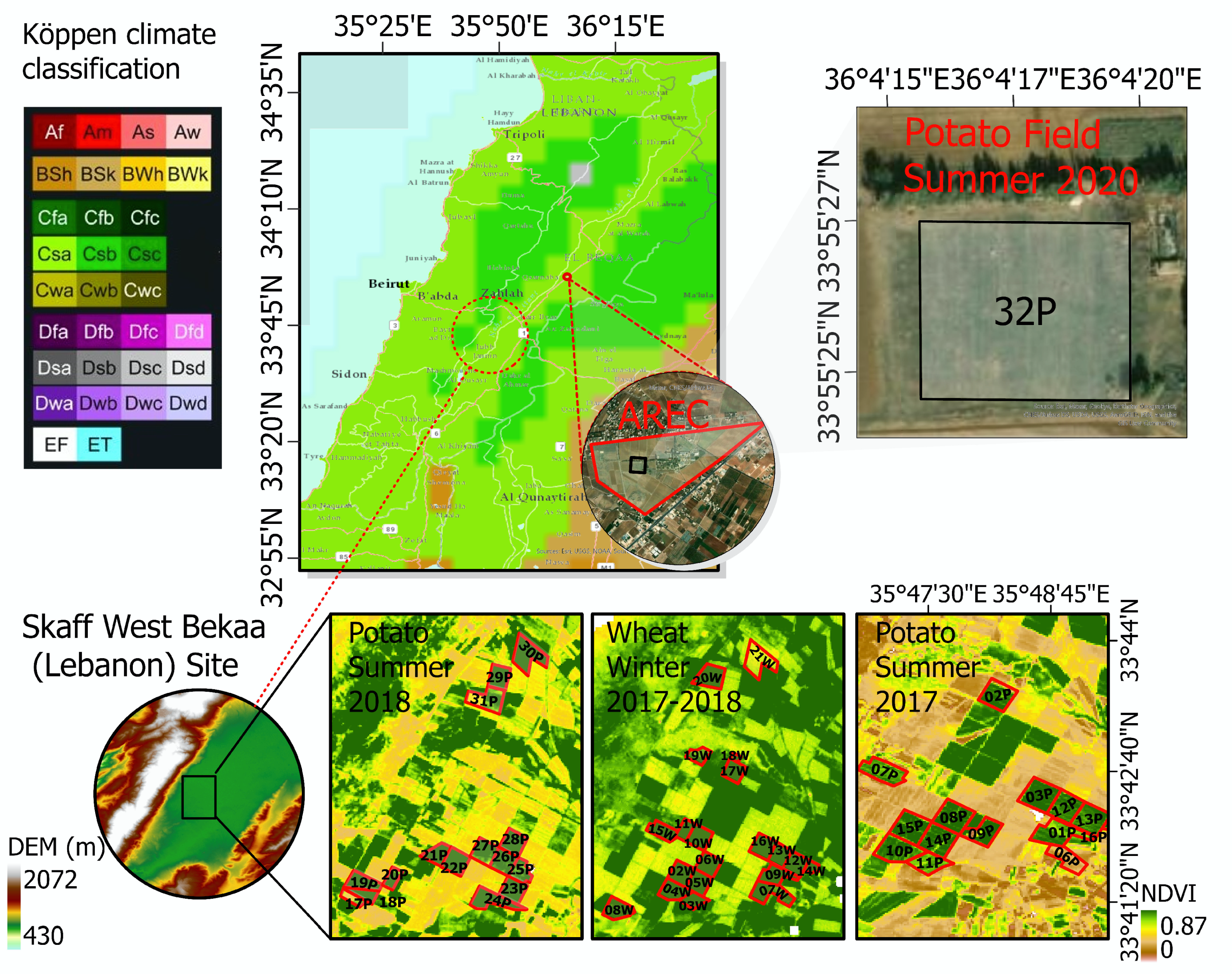
3.2.1. Skaff (Bekaa, Lebanon) Site

The analyzed crops include 21 wheat (T. aestivum) and 31 potato (S. tuberosum) experimental fields located in the west of Bekaa Valley, Lebanon, with an average elevation of 862 m above sea level (Figure 3). According to Köppen’s climatic classification, the climate of the region is Mediterranean (Csa). The predominant soil of the region is fertile clay soil. All fields monitored are irrigated using sprinkler irrigation systems. Management practices follow local practices. Traditional tillage is common. Herbicides are applied once per season for wheat culture and between six and eight times for potato culture. Pesticide spray is carried out at one to two sprays per season, and the fertilizers in the form of urea (43% nitrogen) are applied once, at a rate of minimum 120 kg/ha to a maximum of 800 kg/ha or 336 kg of net N/ha/season for wheat culture, while potato uses 230 kg/ha of nitrogen fertilizer. Potato rotation is widely practiced in West Bekaa (Skaff farms) with wheat, vegetables, and legumes.
The actual yield dataset for the analyzed fields was collected via an interview with the Skaff farms’ farmer-manager. This approach of data acquisition is referred to as the recall method [99]. The data records were obtained on crop maps, areas planted, crop type, and crop yields for three consecutive seasons: summer 2017, summer 2018, and winter 2017–2018. Agronomic measurements for estimating the harvest index (HI) and crop moisture content (%) parameters were conducted for Skaff fields (West Bekaa, Lebanon). These measurements were taken during the late growing season of the crops (May–September 2018) over two potato and three wheat experimental fields located in West Bekaa (Lebanon). The quadrate was randomly thrown in the field, and the vegetation within the frame of the quadrate was clipped. Three samples of the biomass were taken from each field, and the obtained results were averaged. The above-ground plant component was oven-dried at 75 °C for 48 h to a constant weight and weighed. The water content of the plants was determined by subtracting the above-ground dry mass from the fresh above-ground mass. The crop moisture content (%) was determined by dividing the water content by the fresh crop weight. The experimental verification of potato moisture content (%) showed that the percentage moisture content of potato tuber varies between 75% and 78% (Table S1). As for wheat, the moisture content of grains ranged between 12% and 15% (Table S2). In this study, we used a value of 0.75 for the potato HI and 0.4 for the wheat HI (Table 2), as verified by the literature.

3.2.2. AREC (Bekaa, Lebanon) Site

The studied experimental field is located at the American University of Beirut’s Agricultural Research and Education Center (AREC) in Bekaa, Lebanon, a 990 m elevation above sea level. Potato (Spunta variety) was planted on 12 March 2020 in an area of 9468 m2. Fertilizers were applied before planting (50 kg of di-ammonium phosphate (DAP) and 25 kg of potassium sulfate) and during the growing season (50 kg of urea). The field is irrigated using a micro-sprinkler system. For HI and percentage crop moisture content calibration, biomass data were collected weekly from 30 April 2020 until 7 July 2020. A summary of the collected data and calculated parameters is illustrated in Table S3.

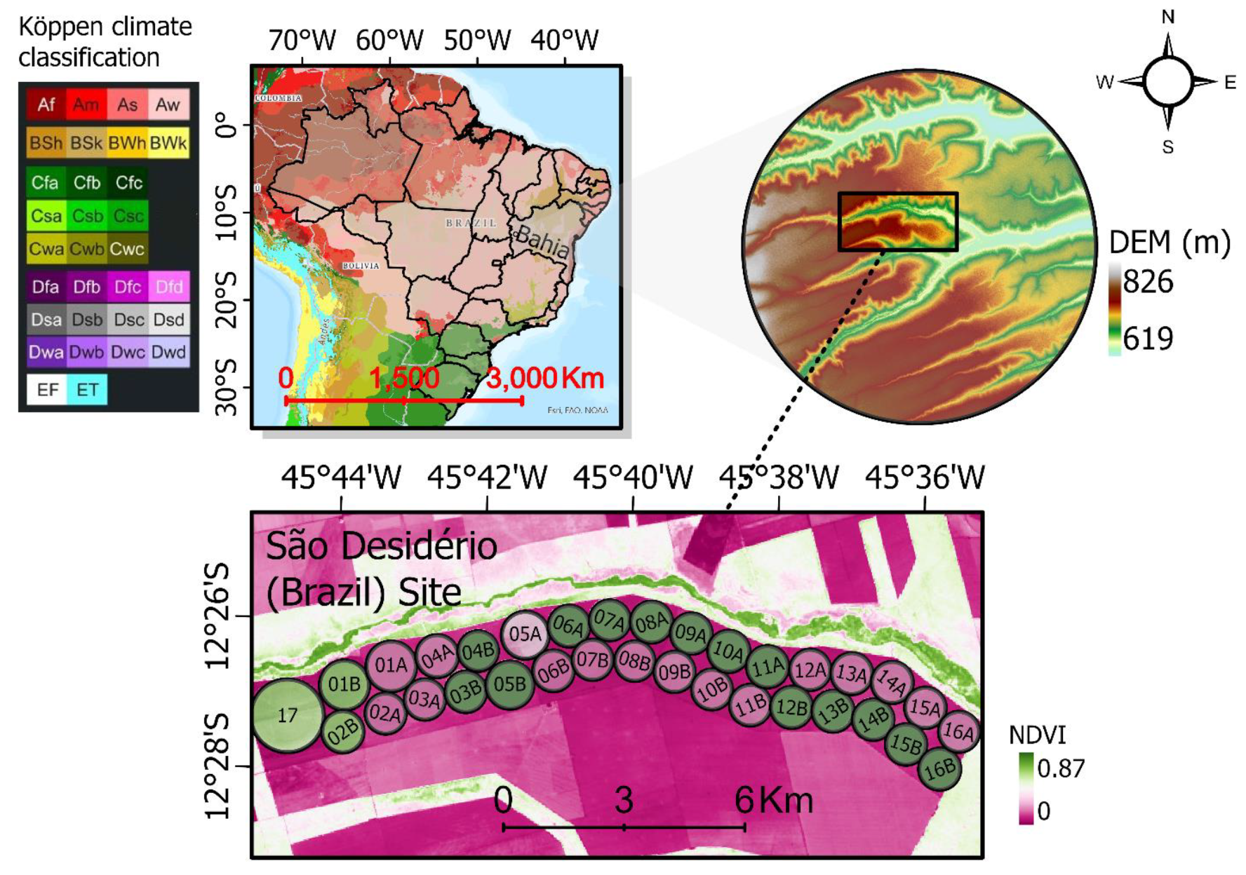
3.2.3. São Desidério (Brazil) Site

The field data used for the Brazil site are for 33 center pivots commercial fields located in the municipality of São Desidério in the western region of the state of Bahia, Brazil. The rectangular area boundary of the analyzed fields is defined by the coordinate pairs 12°28′08″S–45°45′12″W and 12°25′40″S–45°34′55″W, with an average altitude of 750 m above sea level. The predominant soil type of the studied fields is Yellow Latosol [110]. According to Köppen’s climatic classification, the climate of the region is tropical (Aw) characterized by a rainy season in summer and a dry winter, with an annual precipitation of 1003.4 mm (Figure 4). Crop-specific parameters used for yield conversion are given in Table 2.

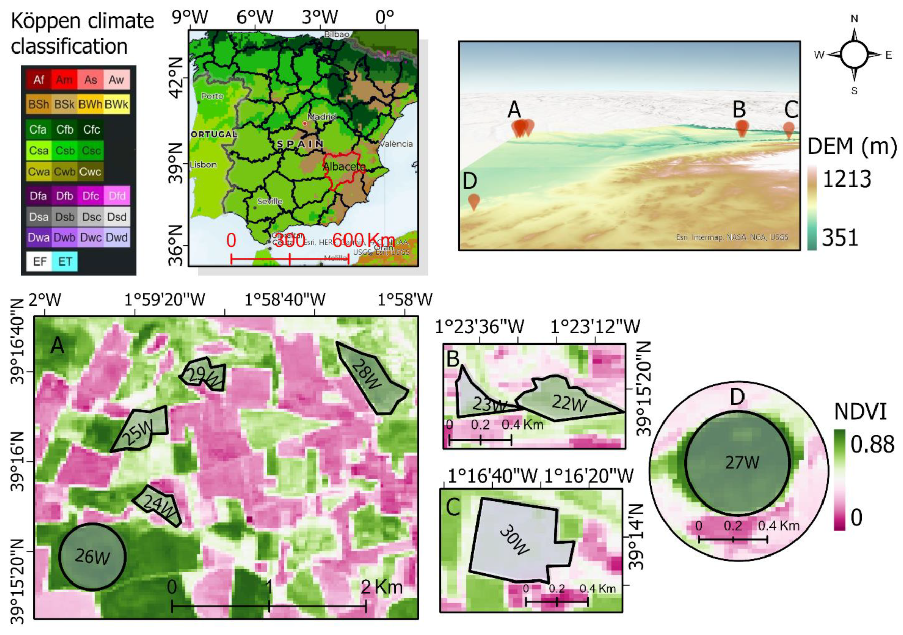
3.2.4. Albacete (Spain) Site

The studied fields are located in the province of Albacete (southeast of Spain). The study site lies at 689 m above sea level, with a prevailing climate considered as BSk according to the Köppen–Geiger climate classification. The annual temperature and precipitation of the study site are 13.6 °C and 340 mm, respectively [96]. The yield data are obtained from commercial wheat fields under irrigated (fields 26W and 27W) and rain-fed conditions for the rest of the analyzed fields (Figure 5). All irrigated fields use center pivot systems. Crop yield data for Fields 22W through 27W were for the 2017 growing season, and 28W through 29W were for the 2018 season. Specific ground measurements of the HI for each field were used, varying from 0.38 to 0.45 [96].

3.3. Datasets

3.3.1. Landsat Surface Reflectance Data

Georeferenced and atmospherically corrected Landsat 7 ETM+ and Landsat 8 OLI/TIRS imagery data were mosaicked, gap-filled (Landsat 7), masked for clouds, and composited within the Google Earth Engine (GEE) platform [111]. For the Skaff (Bekaa, Lebanon) study site, Landsat data with Path 174 Row 37 images for the period 2017–2018 were processed. A total of 27 and 23 nearly cloud-free scenes were used for the 2017 and 2018 growing seasons, respectively. For the AREC (Bekaa, Lebanon) study site, a total of 11 scenes were used to cover the 2020 growing season. For the Brazil site, Landsat WRS-2 Path 220, Row 069 scenes for the corn season (April–October) for 2015 and 2016 each were used. We acquired 40 images of the Brazil study site, including images from both OLI and ETM+sensors for both years. As for the Spain site, a total of 44 images were used for the 2017 growing season and 39 for the 2018 season. The images were selected to cover the full growing season for each culture, with at least four images per field, with an image close to the beginning, middle, and end of the crop cycle to amply define it. The dates with available images are shown in Table S4 (Supplementary Material). Table 3 shows the major data input fed to the tested model with their respective spatial and temporal resolutions, and possible uncertainties.

3.3.2. Weather Data

We use the 6 hr CFSV2 gridded (0.2 arc degrees) weather dataset available in GEE generated by the National Centers for Environmental Prediction (NCEP) of the National Oceanic and Atmospheric Administration (NOAA) [113]. CFSV2 version 2 was developed at the Environmental Modeling Center at the NCEP. CFSV2 is a fully coupled model representing the interaction between Earth’s atmosphere, oceans, land, and sea ice. Currently, CFSV2 is the global weather reanalysis and forecast tool that has the highest temporal and spatial resolution to allow for real-time reference evapotranspiration calculations and forecasts in GEE. Other available datasets or systems (e.g., GLDAS, NASA-POWER, ECMWF) are either not available in near real time in GEE or have a lower resolution. Each grid of the CFSV2 file covers an approximate area of 490 km2. The variables used in the model to calculate ETref and consequently ETact and transpiration are presented in Table 4.

3.4. Definition of the Growing Season

The NDVI time-series images are used to define the crop phenology of each field at pixel scale. An NDVI value of 0.2 is used as an indication of the beginning and the end of the season [114].

3.5. Statistical Indicators

To assess the accuracy of the yield estimations, the statistical indicators root-mean-square error (RMSE), mean absolute error (MAE), mean bias error (MBE), relative error (RE), and index of agreement (d) between the estimated and actual yield values are calculated:
Root-mean-square error (RMSE):
RMSE = i = 1 n ( Estimated   Yield i Reported   Yield i ) 2 n
Mean absolute error (MAE):
MAE = i = 1 n | Estimated   Yield i Reported   Yield i | n
Mean bias error (MBE):
MBE = i = 1 n ( Estimated   Yield i Reported   Yield i ) n
Relative error (%RE):
RE = i = 1 n ( Estimated   Yield i Reported   Yield i ) i = 1 n Reported   Yield i
Index of agreement (d):
d = 1 i = 1 n ( Reported   Yield i Estimated   Yield i ) 2 i = 1 n ( | Estimated   Yield i Reported   Yield i ¯ | + | Reported   Yield i Reported   Yield i ¯ | ) 2

4. Results and Discussion

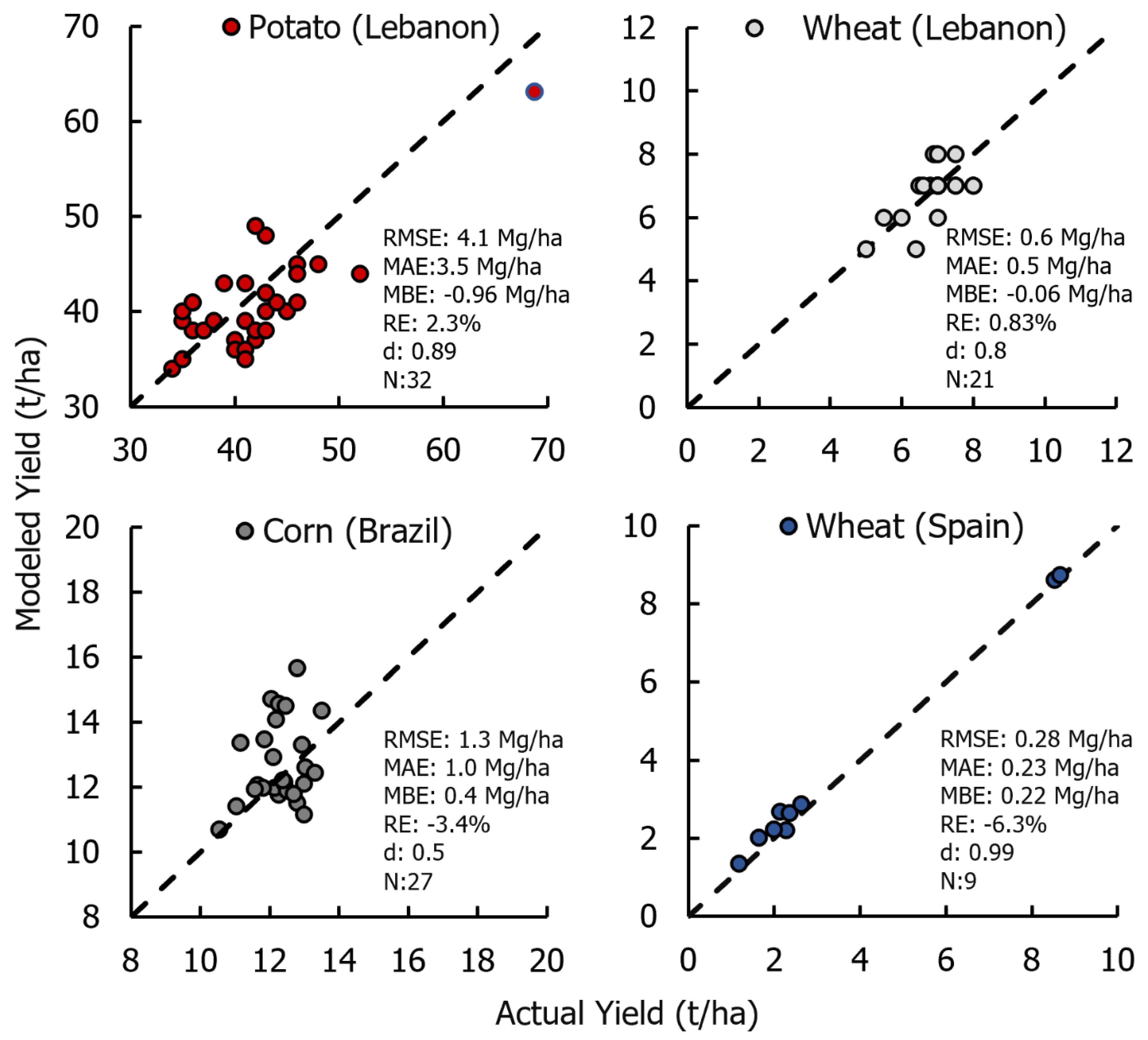
4.1. Model Performance

Figure 6 shows the measured versus estimated corn, wheat, and potato yields for the growing seasons of 2015 and 2016 for corn and 2017 and 2018 for wheat and potato. Potato yield was estimated with a good agreement (d = 0.89, RMSE = 4.1 t/ha, MAE = 3.5 t/ha, MBE = −0.96 t/ha, and RE = only 2.3%). We believe that this difference is within the measurement uncertainty. A comparison of the accuracy of the yield estimation of potato shows that the model performed slightly better in summer 2017 than in summer 2018, with lower RMSE and MAE values (Table 5). The modeled potato yield for the analyzed field in the 2020 growing season at AREC, Bekaa (Lebanon) showed a low deviation from the reported yield, quantified at 8.2%. A better agreement was observed in the wheat crop, and the RMSE (RE) between the measured and simulated values were low (0.6 t/ha (0.83%)), and d was high (0.8), with a slight underestimate of −0.06 t/ha. The accuracy of estimation of the corn grain yields was not as good as that of potato and wheat, but it was acceptable. The index of agreement value (0.5) for the 2015 and 2016 growing season was acceptable, with an RMSE greater than 1 (1.3 t/ha). The RE was −3.4%, with a slight overestimate of 0.4 t/ha, which is considered subtle, and the MAE was equal to 1 t/ha. These values are very satisfactory. The 2016 growing season had six different sown hybrids, which may have contributed to this slight variation due to the use of a single HI (HI = 0.45) for all hybrids. The 2015 growing season had lower values of the RMSE, MAE, MBE, and RE. Additionally, the obtained RMSE in the present study is considered very good in comparison to the results of Sibley [24], where the authors reported RMSE values above 2 t/ha for the verified approach to be promising. Regarding the wheat grain yield at the Albacete study site, the RMSE between the modeled and actual values was 0.28 t/ha, with a slight overestimate of 0.22 t/ha. Additionally, a good agreement existed between the modeled and actual values, with a value of 0.99. Both RMSE and d values were better than those obtained by Campos et al. [115] for their tested approach on wheat fields located in the southeast of Spain, where they showed RMSE values varying between and 0.27 and 1.65 t/ha and the highest d of 0.83.
Figure S3 shows the absolute difference in percentage between estimated and actual yield values for the analyzed crops at a field level. Both wheat and potato at the West Bekaa study site had a percentage difference range of ±16%. Still, most of the percentage differences ranged between ±10%. For corn, the percentage difference in the grain yield ranged between −22.4% and 14.2%. The 2016 growing season had the largest error. The highest difference was observed in 2016 (Pivot 13B), with a value of −22.4%, followed by −18.8% in Field 16B. The 2015growing season had only one value greater than 16%. The Brazil site had more clouds than the other sites, and interpolation between non-cloudy Landsat overpasses will bring more uncertainty for crops with a shorter growing season (corn matures in 90 days). Excluding the fields that had the highest percentage difference, the percentage difference of the remaining fields was within ±16% for both Brazil and Lebanon sites. On the contrary, the modeled yield deviated by an average of −10.9% from the reported yield in only two fields 25W and 22W, having a difference of greater than ±15% at the Albacete (Spain) study site. This can be attributed to the small size of both fields (average area of 11.5 ha) compared to the average combined field sizes of 24 ha (Table 1).

4.2. Within-Field Spatial Variability in Above-Ground Biomass (AGB), Soil Moisture Stress (SMS), and Crop Yield

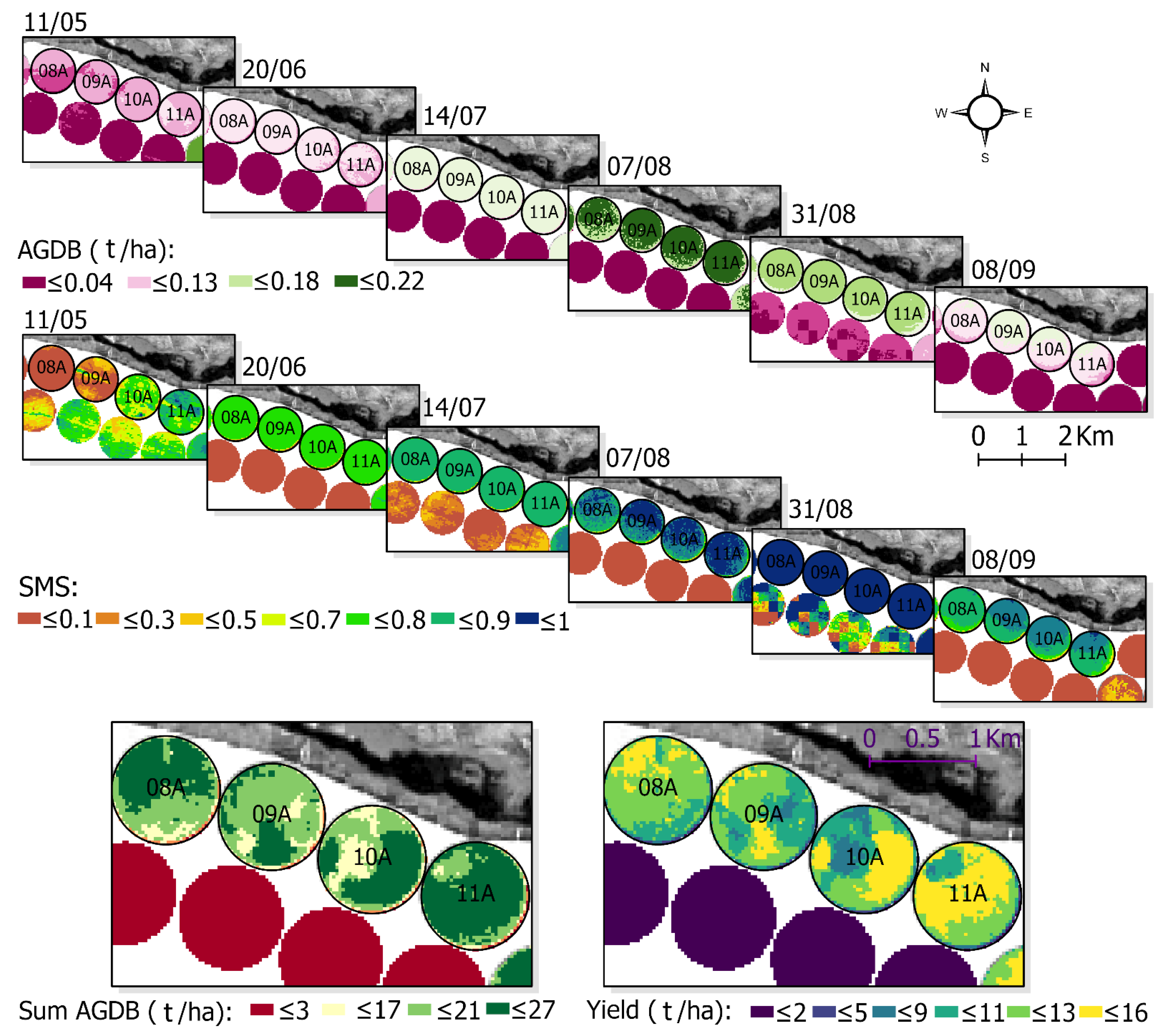
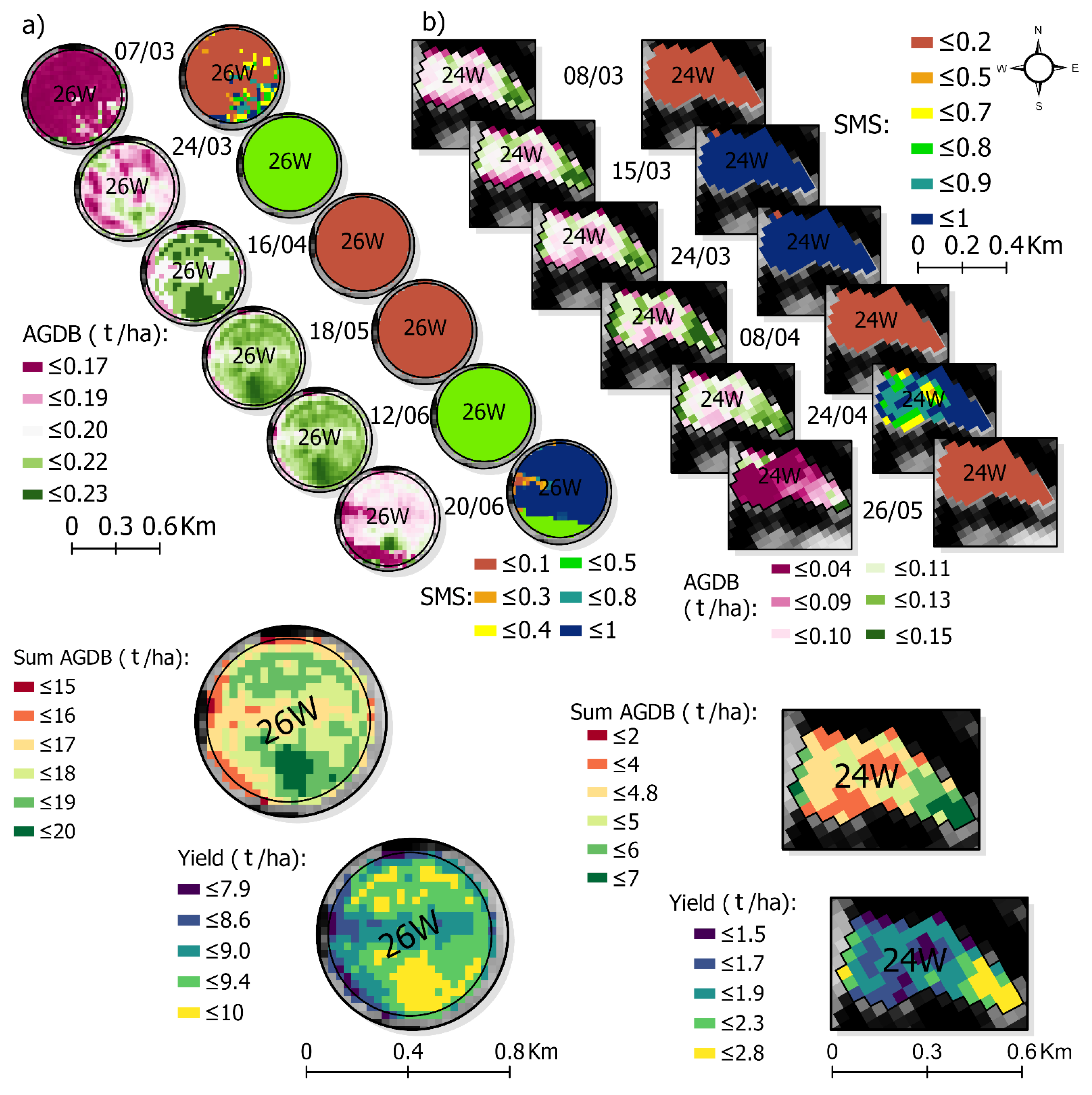
4.2.1. Potato: Skaff (Bekaa, Lebanon) Site

The variations of the AGDB and the soil moisture stress (SMS) scalar at satellite overpasses of the two emphasized potato fields during 2018 result in prominent differences in terms of the accumulated above-ground biomass and yield (Figure 7). A deficit in soil moisture can influence the length of the crop development stages through early crop senescence and thereby reduce the yield. Compared to some studies that neglect the impact of moisture stress when irrigation water is available [116], our analysis indicates that moisture stress represents a major limiting factor for LUEact and crop yields in irrigated fields. Results show that Field 31P had low moisture stress (in the neighborhood of one) throughout the days of the satellite overpass as compared to Field 30P, which experienced some incidents of soil moisture stress (in the neighborhood of zero) during two satellite overpasses (dates 11/03 and 12/04). Some patches of high moisture stress were noticed in Field 31P. Both fields experienced high moisture stress on the day nearest the harvest date (18/08). The high moisture stress observed during the satellite overpass in Field 30P is possibly due to a difference in irrigation time (farmers could have been irrigation past the Landsat overpass time at 10:00 a.m. local time).
An interpretation of the light use efficiency, accumulated AGDB, and the reported and modeled yields between the two selected fields shows significant differences. With the same vapor and temperature stresses over the two fields, we noticed that the mean value of the LUE in Field 30P (1.23 g/MJ) was 12% lower than that in Field 31P. The mean value of the combined stresses was higher in Field 30P (Table 6). The stresses showed up better in the reported yields, with an 11% difference in stress resulting in a 17% difference in yield. The modeled yield was only 3% less, possibly due to the assumption of the linearity in the interpolation between satellite overpasses. Other factors affecting the variation in the AGB and yield estimation are the crop’s susceptibility to unfavorable growth conditions, differences in planting and harvest dates, weed control, and irrigation management. For instance, the presence of abundant weeds in the monitored fields could lead to overestimating biomass production and inaccurate estimation of crop yield.

4.2.2. Corn: São Desidério (Brazil) Site

Figure 8 shows the spatiotemporal distribution of the AGDB and soil moisture stress (SMS) over the corn-growing season (2016). Low biomass values were found in the initial stages (date 11/05) accompanied by high moisture stress due to the large area of uncovered soil in this period. Generally, the SMS values at the satellite overpass for four emphasized center pivots were close to unity, except at the beginning of the growing season after sowing and in the late season. SMS values started to decrease on 08/09 when the irrigation intervals became longer during the physiological maturity phase of corn. Consequently, based on SMS values that remained close to unity, it is evident that cultivated fields did not suffer from water stress and thus obtained high yields. These results are consistent with previous work, showing an average value of the water stress coefficient (0.94) for four selected center pivots monitored in 2016, indicating the low impact of water stress on biomass production [95]. The visual inspection of yield maps reveals that vegetation conditions were slightly variable between the four emphasized fields over the growing season. This could be due to the use of different corn cultivars.

4.2.3. Wheat: Albacete (Spain) Site

The biomass production dynamically changes during the growing cycle due to factors related to meteorological conditions and crop physiology and management [115]. Grown under different management conditions, and with different lengths of the growth cycle, irrigated Field 26W produced a higher accumulated AGDB and yield than rain-fed Field 24W, possibly due to severe water-limited conditions in Field 24W. The growing cycle in irrigated varieties spans from January to the end of June and in rain-fed varieties from November to the end of May. Selected images from the growing cycle over the emphasized fields are displayed in Figure 9. An increase in the AGDB during the development phase of both Fields 24W and 26W was noted, which can be confirmed by the difference between the selected first and last images (dates 07/03 and 20/06 for Field 24W and 08/03 and 26/05 for Field 26W). During the mid-season (dates 24/03 and 24/04 for Field 24W and 18/05 for Field 26W), high values of the AGDB are observed because of the good crop establishment. High soil moisture stress is visible at the initial stages of the growth cycle for both fields (dates 07/03 for Field 24W and 08/03 for Field 26W). Figure 10 shows the possible detection of high soil moisture stress (SMS) within-field variability at Landsat overpasses, evident on 16/04 and 18/05 for Field 26W and 08/04 for Field 24W. This approach can be advantageous for precision irrigation, providing accurate information about irrigation practices, such as water application uniformity and areas with surface runoff or irrigation deficits near the outside borderline of the central pivot systems, which was confirmed in Field 26W on 20/06, suffering from high moisture stress (~0.5) near its outer boundary.

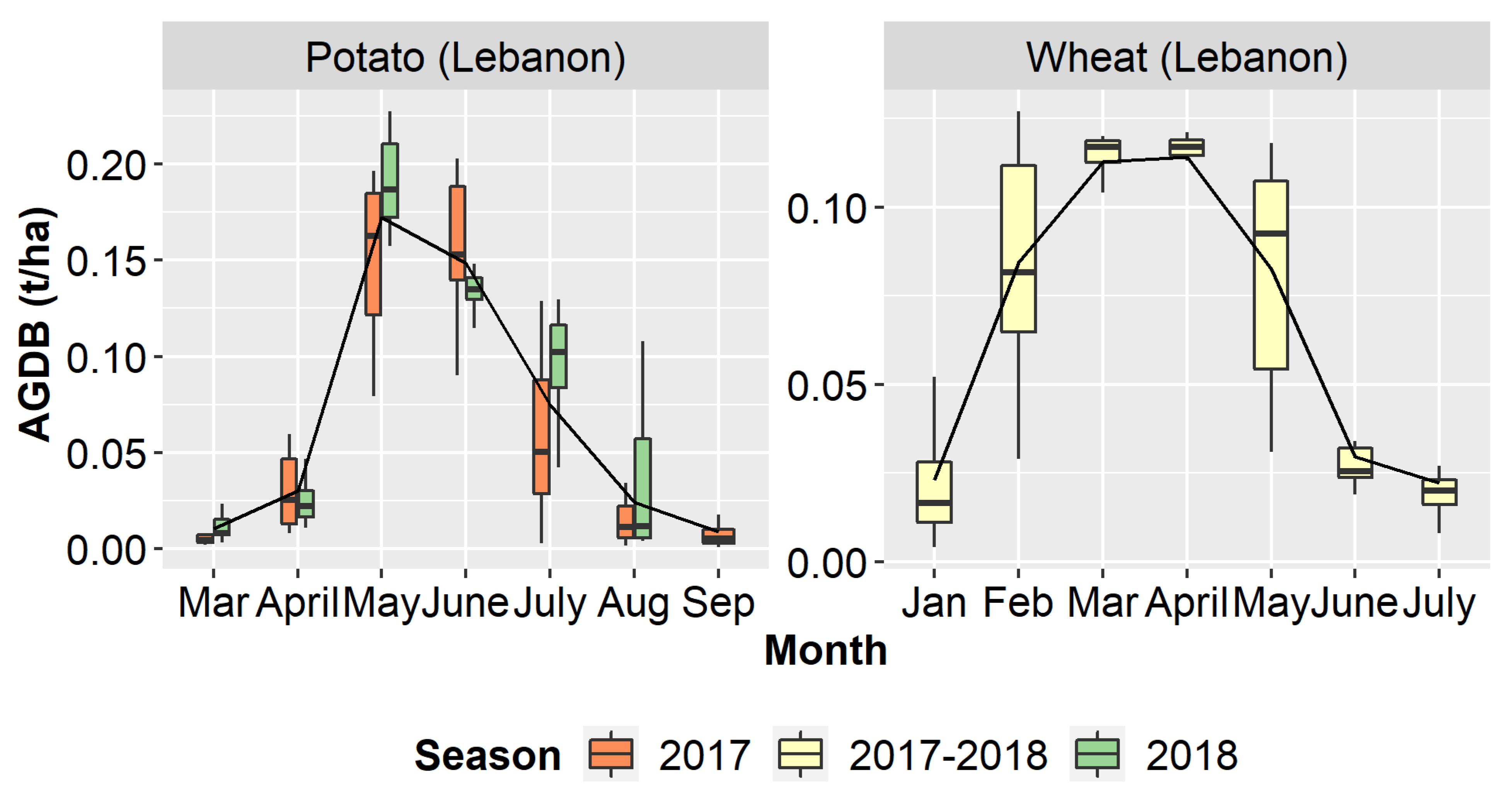
4.3. Seasonal Co-Variability in Above-Ground Dry Biomass (AGDB), Environmental Stressors, and Yield: Examples from Lebanon

Understanding patterns of the AGB is essential for guiding farming practices and helps farmers in decision making. Figure 10 shows the time development of the monthly AGDB. The variability across the months is considerable, reflecting differences in potato and wheat crop phenology. It is possible to detect very similar behaviors for both wheat and potato, with a fast increase in biomass at the start of the growing cycle, stability during the mid-season, and a decrease at the end. The AGDB started to increase in March, and it peaked in May (middle of the season) at ~0.2 t/ha. A decrease in the monthly AGDB was noticed at the end of the growing season in August. As for wheat, the monthly biomass reached its maximum in March–April, at ~0.12 t/ha, and then decreased toward the end of the growing season (June–July).
The potato crop in the Bekaa site diverged in its AGDB temporal profile in the 2017 and 2018 growing seasons. These deviations can be attributed to the variation of environmental stressors among the seasons of the same crops. To study the impact of the environmental stressors, an inter-comparison between seasons was performed. Our analysis shows that the soil moisture, temperature, and combined stresses were higher in summer 2017 as compared to 2018 (Table 7). This was notable in terms of the maximum actual LUE and the AGDB for potato in summer 2018, which were, respectively, 5% and 10% higher than those in 2017 (due to higher moisture and temperature stress). Furthermore, the average modeled and reported yields for potato in 2018 were 9% and 6% higher than those in 2017, respectively. In contrast to potato crop, wheat crop studied during winter 2017–2018 experienced lower environmental stresses (with values approaching unity, indicating low stress). This is evident in terms of a higher average combined stress factor and lower moisture stress (Table 7).

4.4. Assessment of the Operational Model: Strengths and Weaknesses

Our work’s breakthrough is that it is the first to provide 30 m crop biomass with relatively high spatial and temporal resolution using soil and weather data along with ET data generated in the same model. GYMEE is highly adaptable, and it can ingest Sentinel-2 multispectral imagery and the VIIRS-375 m I-5 thermal band, allowing even for higher spatial (10 m) and temporal (2–3 days) resolution. It can also adapt to various single- and dual-source energy balance ET models, such SSEB, SEBS, and TSEB. A crop-specific LUEmax should be utilized whenever crop data are known. Given that there is no consensus in the scientific community on the maximum LUE for even the same crop (see, for example, Chen et al. [117] and Zhu et al. [118]) and given that GYMEE performed very well with these average values, we believe that the two values (2.5 for C3 and 3.5 for C4) provide good enough estimates for modeling the biomass using the Monteith equation. The LUEmax parameterization might introduce some uncertainty, but we believe that it is a strength of the model that it performed very well with the average values of LUEmax. It would be straightforward to update GYMEE with a LUEmax map derived from a crop map when such a map becomes available. At present, many global products for land-cover classification are available, which only provide information for broad classes, such as forest, cropland, and grassland, but not crop types. The dynamic nature of cropping patterns and within-year variations needs to be considered since this is a field-scale model. The analyses performed consider different physical soil properties by using global gridded soil data from an Open Land Map Earth Engine dataset Hengl and MacMillan [85] available in GEE. Additionally, the proposed operational model considers the variations in environmental conditions by incorporating environmental stresses (temperature, vapor, and soil moisture constraints) computed from agrometeorological data of the global 6 h CFSV2 gridded weather dataset available in GEE. The proposed model’s major operational advantage is the spatial quantification of the soil moisture stress constraint and its impact on reducing biomass production. This approach can be alternatively used for areas with limited ground data availability.
There are a few uncertainties for simulating the AGB as well as crop yield, including uncertainties of satellite data and model parameters. We use multispectral VIs to determine the length of the growing cycle. However, this approach is limited under cloudy conditions. Future implementations could harness NDVI-S1 radar data relationships to fill in long gaps over cloudy regions. In addition, if a scene is missed due to clouds, the small temporal resolution (say 16 days) under water deficit conditions could lead to inaccurate biomass values [119]. In these situations, the use of different thermal times like growing-degree-days and accumulated reference evapotranspiration (ETref) with the temporal evolution of VIs to monitor phenology could be an alternative [120]. The parameterization of the LAI and the fPAR would also bring some uncertainty as there is no consensus in the literature on a physical method to derive the LAI from remote sensing [121]. Even though the percentage difference between the modeled and actual yields is considered low (Figure 7), the prediction may be improved by using crop-specific parameters (harvest index and percentage moisture content of produce) instead of single values. It is vital to use different HIs when considering different hybrids and years under various weather environments [95]. Crop yield varies with the crop’s moisture content (percentage moisture) at harvest and with the HI. The HI varies with the variety of the crop and the cultural practices, and therefore a range should be provided. Careful estimation of the HI and the percentage moisture is necessary to derive accurate yields from biomass calculations. For example, a high-yielding variety of the same crop would have a higher HI. GYMEE does not predict the HI or the percentage moisture, both of which should be specified by the user to derive the yield from the biomass. Other uncertainties could arise from the constants in the heat stress equation. A sensitivity analysis of the response of the heat stress to changes in the parameters is presented in Figure S4 (Supplementary Material). With the simulated results, it can be deduced that both values of optimal conductance temperature and temperature stress scalar would have had a low uncertainty for the crop yield estimation. Of course, model performance could be better with optimized TH and KT values specific to each crop type.
Some uncertainty, which is not due to the model itself, might arise from actual crop yield data acquisition. For example, we used the recall method for the Skaff (Bekaa, Lebanon) site. Although this approach produced good results, it may include uncertainty if farmers over- or under-report their crop yields or when farmers do not account for within-field variability as they provide values on a whole-plot basis [99,122]. Other sources of error, not directly attributable to the model, are issues due to the size and shape of the fields. Overall, the poorest performance was obtained in small fields (Fields 25W and 22W from the Spain study site), with an average size less than 12 ha. The accuracy of the yield estimation is affected in small fields [123], and here Sentinel-2 can be used. The model is also sensitive to landscape evaporation. Using an ET model other than the modified pySEBAL might yield is a different transpiration component that would influence the soil moisture stress scalar of the yield. An ensemble of ET models may be a better approach. In fact, we have already started implementing GYMEE using a harmonized Landsat–Sentinel-2 product and sharpened thermal bands of MODIS and VIIRS, along with a more stable energy balance model.

5. Conclusions

In this study, a newly proposed GYMEE model for predicting yield at the farm level, based on the integration of ET and abiotic stressors into the light use efficiency and Monteith model, was presented and evaluated using surface reflectance images from Landsat 7 and 8 satellites. GYMEE shows promising results in running within the GEE platform. GYMEE was validated at different sites (Lebanon, Spain, and Brazil) for wheat, potato, and corn. The results obtained in the present work endorse the use of remote sensing as a helpful tool for the operational estimation of crop yield at a field scale under a wide range of ecology, management systems, and soil types. Compared to the literature, this research focuses on the following aspects: (i) spatio-temporal crop yield modeling at the small field scale under a wide range of management conditions, (ii) an operational framework for crop yield modeling, and (iii) integration of global weather data (CFSV2) and global soil data into actual evapotranspiration and abiotic stressor calculations for biomass calculations. Because it is implemented in GEE, GYMME can be used to estimate the ET at the global scale and improve the understanding of water use by crops as well as improve estimates of the ET as a major component of the hydrologic cycle. As more soil moisture products become, available either via further analysis of radar data, such as Sentinel-1, or via downscaling of existing soil moisture missions such as Soil Moisture Active Passive (SMAP), a more comprehensive sensitivity analysis becomes possible for validating the model in other areas of the world where yield data are available. We conclude that the suggested method can be a useful tool for estimating the yield of the studied crops in Mediterranean, semi-arid, and tropical climates.

Supplementary Materials

The following are available online at https://www.mdpi.com/2072-4292/13/4/773/s1: Table S1: Agronomic measurements for potato crop at Skaff (West Bekaa, Lebanon) (average of three samples for each date), Table S2: Agronomic measurements for wheat at Skaff (West Bekaa, Lebanon) (average of three samples for each date), Table S3: Agronomic measurements for potato at AREC (Bekaa, Lebanon), Table S4: At-site cloud-free Landsat imagery used in this study, with respective dates; L7 (Landsat 7) and L8 (Landsat 8); Figure S1: Wheat-fields NDVI time series Plots for winter 2017–2018 season, Figure S2: Potato fields NDVI time series plots for the summer 2018 season, Figure S3: Percentage deviation (%) of modeled yield from the actual yield for the analyzed crops at each of the studied sites, Figure S4: Simulations of temperature stress (TS) at a fixed daily air temperature of (28 °C) as a function of: (a) the upper limit of stomatal activity (°C) (TH) and (b) the optimum conductance temperature (°C) (KT).

Author Contributions

Conceptualization, H.J.; methodology, H.J.; validation, H.J. and R.M.; formal analysis, H.J. and R.M.; investigation, H.J. and R.M.; resources, H.J.; data curation, H.J. and R.M.; writing—original draft preparation, H.J. and R.M.; writing—review and editing, H.J.; visualization, R.M.; supervision, H.J.; project administration, H.J.; funding acquisition, H.J. All authors have read and agreed to the published version of the manuscript.

Funding

This research was funded by a grant from NASA, grant number 17-LCLUC17-0002- 08NSSC18K0483 under the project Characterizing Field-Scale Water Use, Phenology and Productivity in Agricultural Landscapes using Multi-Sensor Data Fusion” and IHE Delft Partnership Programme for Water and Development (DUPC2)—the Netherlands Ministry of Foreign Affairs, grant number 103768, under the project “ITSET: Integrating time-series ET mapping into an operational irrigation management framework”. Support from the American University of Beirut Research Board (URB)—Award 103795 is also acknowledged.

Institutional Review Board Statement

Not applicable.

Informed Consent Statement

Not applicable.

Data Availability Statement

Publicly available datasets were analyzed in this study. This data can be found here: [https://earthengine.google.com] (accessed on 1 August 2020).

Acknowledgments

Special thanks to Naji Beyrouthy for helping in coding, field data collection, and data export. We also thank Mohammad Ali Jaafar for providing access to his fields in Bekaa.

Conflicts of Interest

The authors declare no conflict of interest. The funders had no role in the design of the study; in the collection, analyses, or interpretation of data; in the writing of the manuscript; or in the decision to publish the results.

References

  1. Khaki, S.; Wang, L. Crop yield prediction using deep neural networks. Front. Plant Sci. 2019, 10, 621. [Google Scholar] [CrossRef] [PubMed] [Green Version]
  2. Kross, A.; McNairn, H.; Lapen, D.; Sunohara, M.; Champagne, C. Assessment of RapidEye vegetation indices for estimation of leaf area index and biomass in corn and soybean crops. Int. J. Appl. Earth Obs. Geoinf. 2015, 34, 235–248. [Google Scholar] [CrossRef] [Green Version]
  3. Scharf, P.C.; Lory, J.A. Calibrating corn color from aerial photographs to predict sidedress nitrogen need. Agron. J. 2002, 94, 397–404. [Google Scholar] [CrossRef]
  4. Bastiaanssen, W.G.; Molden, D.J.; Makin, I.W. Remote sensing for irrigated agriculture: Examples from research and possible applications. Agric. Water Manag. 2000, 46, 137–155. [Google Scholar] [CrossRef]
  5. Mahlein, A.K.; Oerke, E.-C.; Steiner, U.; Dehne, H.W. Recent advances in sensing plant diseases for precision crop protection. Eur. J. Plant Pathol. 2012, 133, 197–209. [Google Scholar] [CrossRef]
  6. Dorward, A.; Chirwa, E. A Review of Methods for Estimating Yield and Production Impacts. 2010. Available online: https://eprints.soas.ac.uk/16731/1/FISP%20Production%20Methodologies%20review%20Dec%20Final.pdf (accessed on 19 February 2021).
  7. Rauff, K.O.; Bello, R. A review of crop growth simulation models as tools for agricultural meteorology. Agric. Sci. 2015, 6, 1098. [Google Scholar] [CrossRef]
  8. Tiwari, P.; Shukla, P.K. A Review on Various Features and Techniques of Crop Yield Prediction Using Geo-Spatial Data. Int. J. Organ. Collect. Intell. (IJOCI) 2019, 9, 37–50. [Google Scholar] [CrossRef]
  9. Chlingaryan, A.; Sukkarieh, S.; Whelan, B. Machine learning approaches for crop yield prediction and nitrogen status estimation in precision agriculture: A review. Comput. Electron. Agric. 2018, 151, 61–69. [Google Scholar] [CrossRef]
  10. Reynolds, C.A.; Yitayew, M.; Slack, D.C.; Hutchinson, C.F.; Huete, A.; Petersen, M.S. Estimating crop yields and production by integrating the FAO Crop Specific Water Balance model with real-time satellite data and ground-based ancillary data. Int. J. Remote Sens. 2000, 21, 3487–3508. [Google Scholar] [CrossRef]
  11. Khan, A.; Stöckle, C.O.; Nelson, R.L.; Peters, T.; Adam, J.C.; Lamb, B.; Chi, J.; Waldo, S. Estimating Biomass and Yield Using METRIC Evapotranspiration and Simple Growth Algorithms. Agron. J. 2019, 111, 536–544. [Google Scholar] [CrossRef] [Green Version]
  12. Asseng, S.; Ewert, F.; Rosenzweig, C.; Jones, J.W.; Hatfield, J.L.; Ruane, A.C.; Boote, K.J.; Thorburn, P.J.; Rötter, R.P.; Cammarano, D.; et al. Uncertainty in simulating wheat yields under climate change. Nat. Clim. Chang. 2013, 3, 827. [Google Scholar] [CrossRef] [Green Version]
  13. Hoogenboom, G. Contribution of agrometeorology to the simulation of crop production and its applications. Agric. For. Meteorol. 2000, 103, 137–157. [Google Scholar] [CrossRef]
  14. Steduto, P.; Albrizio, R. Resource use efficiency of field-grown sunflower, sorghum, wheat and chickpea: II. Water use efficiency and comparison with radiation use efficiency. Agric. For. Meteorol. 2005, 130, 269–281. [Google Scholar] [CrossRef]
  15. Jones, C.A. CERES-Maize: A Simulation Model of Maize Growth and Development; Texas A&M University Press: College Station, TX, USA, 1986. [Google Scholar]
  16. Williams, J.R.; Jones, C.A.; Dyke, P.T. The EPIC model and its application. In Proceedings of the International Symposium on Minimum Data Sets for Agrotechnology Transfer, Patancheru, India, 21–26 March 1983; pp. 111–121. [Google Scholar]
  17. Jones, J.W.; Hoogenboom, G.; Porter, C.H.; Boote, K.J.; Batchelor, W.D.; Hunt, L.; Wilkens, P.W.; Singh, U.; Gijsman, A.J.; Ritchie, J.T. The DSSAT cropping system model. Eur. J. Agron. 2003, 18, 235–265. [Google Scholar] [CrossRef]
  18. Steduto, P.; Raes, D.; Hsiao, T.C.; Fereres, E.; Heng, L.K.; Howell, T.A.; Evett, S.R.; Rojas-Lara, B.A.; Farahani, H.J.; Izzi, G.; et al. Concepts and applications of AquaCrop: The FAO crop water productivity model. In Crop Modeling and Decision Support; Springer: Berlin, Germany, 2009; pp. 175–191. [Google Scholar]
  19. Stockle, C.O.; Martin, S.A.; Campbell, G.S. CropSyst, a cropping systems simulation model: Water/nitrogen budgets and crop yield. Agric. Syst. 1994, 46, 335–359. [Google Scholar] [CrossRef]
  20. Boote, K.J.; Jones, J.W.; Pickering, N.B. Potential uses and limitations of crop models. Agron. J. 1996, 88, 704–716. [Google Scholar] [CrossRef]
  21. Dente, L.; Satalino, G.; Mattia, F.; Rinaldi, M. Assimilation of leaf area index derived from ASAR and MERIS data into CERES-Wheat model to map wheat yield. Remote Sens. Environ. 2008, 112, 1395–1407. [Google Scholar] [CrossRef]
  22. Ines, A.V.; Das, N.N.; Hansen, J.W.; Njoku, E.G. Assimilation of remotely sensed soil moisture and vegetation with a crop simulation model for maize yield prediction. Remote Sens. Environ. 2013, 138, 149–164. [Google Scholar] [CrossRef] [Green Version]
  23. Maas, S. Using satellite data to improve model estimates of crop yield. Agron. J. 1988, 80, 655–662. [Google Scholar] [CrossRef]
  24. Sibley, A.M.; Grassini, P.; Thomas, N.E.; Cassman, K.G.; Lobell, D.B. Testing remote sensing approaches for assessing yield variability among maize fields. Agron. J. 2014, 106, 24–32. [Google Scholar] [CrossRef]
  25. Groten, S. NDVI—Crop monitoring and early yield assessment of Burkina Faso. Remote Sens. 1993, 14, 1495–1515. [Google Scholar] [CrossRef]
  26. Sharma, T.; Sudha, K.; Ravi, N.; Navalgund, R.; Tomar, K.; Chakravarty, N.; Das, D. Procedures for wheat yield prediction using Landsat MSS and IRS-1 A data. Int. J. Remote Sens. 1993, 14, 2509–2518. [Google Scholar] [CrossRef]
  27. Monteith, J. Solar radiation and productivity in tropical ecosystems. J. Appl. Ecol. 1972, 9, 747–766. [Google Scholar] [CrossRef] [Green Version]
  28. Daughtry, C.; Gallo, K.; Goward, S.; Prince, S.; Kustas, W. Spectral estimates of absorbed radiation and phytomass production in corn and soybean canopies. Remote Sens. Environ. 1992, 39, 141–152. [Google Scholar] [CrossRef]
  29. Kumar, M. Remote Sensing of Crop Growth. In Plants and the Daylight Spectrum: Proceedings of the First International Symposium of the British Photobiology Society, Leicester, UK, 5–8 January 1981; Smith, H., Ed.; Academic Press: Cambridge, MA, USA, 1981; Volume 1, pp. 133–144. [Google Scholar]
  30. Boschetti, M.; Stroppiana, D.; Confalonieri, R.; Brivio, P.A.; Crema, A.; Bocchi, S. Estimation of rice production at regional scale with a Light Use Efficiency model and MODIS time series. Ital. J. Remote Sens. Riv. Ital. Di Telerilevamento 2011, 43, 63–81. [Google Scholar] [CrossRef]
  31. Patel, N.; Bhattacharjee, B.; Mohammed, A.; Tanupriya, B.; Saha, S. Remote sensing of regional yield assessment of wheat in Haryana, India. Int. J. Remote Sens. 2006, 27, 4071–4090. [Google Scholar] [CrossRef]
  32. Bastiaanssen, W.G.; Ali, S. A new crop yield forecasting model based on satellite measurements applied across the Indus Basin, Pakistan. Agric. Ecosyst. Environ. 2003, 94, 321–340. [Google Scholar] [CrossRef]
  33. Pan, G.; Sun, G.-J.; Li, F.-M. Using QuickBird imagery and a production efficiency model to improve crop yield estimation in the semi-arid hilly Loess Plateau, China. Environ. Model. Softw. 2009, 24, 510–516. [Google Scholar] [CrossRef]
  34. Campos, I.; Neale, C.M.; Arkebauer, T.J.; Suyker, A.E.; Gonçalves, I.Z. Water productivity and crop yield: A simplified remote sensing driven operational approach. Agric. For. Meteorol. 2018, 249, 501–511. [Google Scholar] [CrossRef]
  35. Tawk, S.T.; Chedid, M.; Chalak, A.; Karam, S.; Hamadeh, S.K. Challenges and Sustainability of Wheat Production in a Levantine Breadbasket. J. Agric. Food Syst. Community Dev. 2019, 8, 193–209. [Google Scholar] [CrossRef]
  36. Jaafar, H.; King-Okumu, C.; Haj-Hassan, M.; Abdallah, C.; El-Korek, N.; Ahmad, F. Water Resources within the Upper Orontes and Litani Basins; International Institute for Environment and Development: London, UK, 2016. [Google Scholar]
  37. Ministry of Agriculture. Recensement Generale. In FAO/Project Recensement Agricole; Lebanese Ministry of Agriculture: Bir Hasan, Lebanon, 2012. [Google Scholar]
  38. Darwish, T.; Fadel, A.; Baydoun, S.; Jomaa, I.; Awad, M.; Hammoud, Z.; Halablab, O.; Atallah, T. Potato Performance under Different Potassium Levels and Deficit Irrigation in Dry Sub-Humid Mediterranean Conditions; International Potash Institute (IPI): Zug, Switzerland, 2015; pp. 14–35. [Google Scholar]
  39. AIBA. Agricultural Yearbook of Western Bahia Region—Crop 2016/2017; Barreiras, Brazil, 2017. Available online: http://aiba.org.br/wp-content/uploads/2018/06/anuario-16-17.pdf (accessed on 25 November 2020).
  40. Field, C.B.; Randerson, J.T.; Malmström, C.M. Global net primary production: Combining ecology and remote sensing. Remote Sens. Environ. 1995, 51, 74–88. [Google Scholar] [CrossRef] [Green Version]
  41. De Oliveira Ferreira Silva, C.; Lilla Manzione, R.; Albuquerque Filho, J.L. Large-Scale Spatial Modeling of Crop Coefficient and Biomass Production in Agroecosystems in Southeast Brazil. Horticulturae 2018, 4, 44. [Google Scholar] [CrossRef] [Green Version]
  42. Casanova, D.; Epema, G.; Goudriaan, J. Monitoring rice reflectance at field level for estimating biomass and LAI. Field Crop. Res. 1998, 55, 83–92. [Google Scholar] [CrossRef]
  43. Christensen, S.; Goudriaan, J. Deriving light interception and biomass from spectral reflectance ratio. Remote Sens. Environ. 1993, 43, 87–95. [Google Scholar] [CrossRef]
  44. Garcia, R.; Kanemasu, E.T.; Blad, B.L.; Bauer, A.; Hatfield, J.L.; Major, D.J.; Reginato, R.J.; Hubbard, K.G. Interception and use efficiency of light in winter wheat under different nitrogen regimes. Agric. For. Meteorol. 1988, 44, 175–186. [Google Scholar] [CrossRef]
  45. Rochette, P.; Desjardins, R.L.; Pattey, E.; Lessard, R. Crop net carbon dioxide exchange rate and radiation use efficiency in soybean. Agron. J. 1995, 87, 22–28. [Google Scholar] [CrossRef]
  46. Richards, R.; Townley-Smith, T. Variation in leaf area development and its effect on water use, yield and harvest index of droughted wheat. Aust. J. Agric. Res. 1987, 38, 983–992. [Google Scholar] [CrossRef]
  47. Varlet-Grancher, C.B.; Bonhomme, R.; Chartier, M.; Artis, P. Efficience de la conversion de l’énergie solaire par un couvert végétal. Acta Oecologica Oecologia Plantarum 1982, 3, 3–26. [Google Scholar]
  48. Das, D.; Mishra, K.; Kalra, N. Assessing growth and yield of wheat using remotely-sensed canopy temperature and spectral indices. Int. J. Remote Sens. 1993, 14, 3081–3092. [Google Scholar] [CrossRef]
  49. Calera, A.; González-Piqueras, J.; Melia, J. Monitoring barley and corn growth from remote sensing data at field scale. Int. J. Remote Sens. 2004, 25, 97–109. [Google Scholar] [CrossRef]
  50. Hatfield, J.; Asrar, G.; Kanemasu, E.T. Intercepted photosynthetically active radiation estimated by spectral reflectance. Remote Sens. Environ. 1984, 14, 65–75. [Google Scholar] [CrossRef]
  51. Asrar, G.; Myneni, R.; Choudhury, B. Spatial heterogeneity in vegetation canopies and remote sensing of absorbed photosynthetically active radiation: A modeling study. Remote Sens. Environ. 1992, 41, 85–103. [Google Scholar] [CrossRef]
  52. Carlson, T.N.; Ripley, D.A. On the relation between NDVI, fractional vegetation cover, and leaf area index. Remote Sens. Environ. 1997, 62, 241–252. [Google Scholar] [CrossRef]
  53. Gao, Z.; Xie, X.; Gao, W.; Chang, N.-B. Spatial analysis of terrain-impacted Photosynthetic Active Radiation (PAR) using MODIS data. GIScience Remote Sens. 2011, 48, 501–521. [Google Scholar] [CrossRef]
  54. McCree, K.J. Photosynthetically active radiation. In Physiological Plant Ecology I; Springer: Berlin, Germany, 1981; pp. 41–55. [Google Scholar]
  55. Duffie, J.A.; Beckman, W.A. Solar Engineering of Thermal Processes; John Willey & Sons: New York, NY, USA, 1980. [Google Scholar]
  56. Fletcher, A.L.; Sinclair, T.R.; Allen, L.H., Jr. Transpiration responses to vapor pressure deficit in well watered ‘slow-wilting’and commercial soybean. Environ. Exp. Bot. 2007, 61, 145–151. [Google Scholar] [CrossRef]
  57. Fuchs, M.; Stanghellini, C. The functional dependence of canopy conductance on water vapor pressure deficit revisited. Int. J. Biometeorol. 2018, 62, 1211–1220. [Google Scholar] [CrossRef] [PubMed]
  58. Oren, R.; Sperry, J.; Katul, G.; Pataki, D.; Ewers, B.; Phillips, N.; Schäfer, K. Survey and synthesis of intra-and interspecific variation in stomatal sensitivity to vapour pressure deficit. Plant Cell Environ. 1999, 22, 1515–1526. [Google Scholar] [CrossRef] [Green Version]
  59. Rawson, H.; Begg, J.; Woodward, R. The effect of atmospheric humidity on photosynthesis, transpiration and water use efficiency of leaves of several plant species. Planta 1977, 134, 5–10. [Google Scholar] [CrossRef]
  60. Yuan, W.; Zheng, Y.; Piao, S.; Ciais, P.; Lombardozzi, D.; Wang, Y.; Ryu, Y.; Chen, G.; Dong, W.; Hu, Z. Increased atmospheric vapor pressure deficit reduces global vegetation growth. Sci. Adv. 2019, 5, eaax1396. [Google Scholar] [CrossRef] [Green Version]
  61. Stewart, J. Modelling surface conductance of pine forest. Agric. For. Meteorol. 1988, 43, 19–35. [Google Scholar] [CrossRef]
  62. Stewart, J. On the use of the Penrnan-Monteith equation for determining area évapotranspiration. Estimation Areal Evapotranspiration 1987, 3–12. [Google Scholar]
  63. Jarvis, P. The interpretation of the variations in leaf water potential and stomatal conductance found in canopies in the field. Philos. Trans. R. Soc. Lond. B Biol. Sci. 1976, 273, 593–610. [Google Scholar] [CrossRef]
  64. Ritchie, J.T.; Nesmith, D.S. Temperature and crop development. In Modeling Plant and Soil Systems; Amer Society of Agronomy: Madison, WI, USA, 1991; pp. 5–29. [Google Scholar] [CrossRef]
  65. Maidment, D.R. Handbook of Hydrology; McGraw-Hill: New York, NY, USA, 1993; Volume 9780070. [Google Scholar]
  66. Mishra, V.; Cruise, J.F.; Mecikalski, J.R.; Hain, C.R.; Anderson, M.C. A remote-sensing driven tool for estimating crop stress and yields. Remote Sens. 2013, 5, 3331–3356. [Google Scholar] [CrossRef] [Green Version]
  67. Tadesse, T.; Senay, G.B.; Berhan, G.; Regassa, T.; Beyene, S. Evaluating a satellite-based seasonal evapotranspiration product and identifying its relationship with other satellite-derived products and crop yield: A case study for Ethiopia. Int. J. Appl. Earth Obs. Geoinf. 2015, 40, 39–54. [Google Scholar] [CrossRef] [Green Version]
  68. Teixeira, D.C.; Antônio, H.; Scherer-Warren, M.; Hernandez, F.B.; Andrade, R.G.; Leivas, J.F. Large-scale water productivity assessments with MODIS images in a changing semi-arid environment: A Brazilian case study. Remote Sens. 2013, 5, 5783–5804. [Google Scholar] [CrossRef] [Green Version]
  69. Boulet, G.; Delogu, E.; Saadi, S.; Chebbi, W.; Olioso, A.; Mougenot, B.; Fanise, P.; Lili-Chabaane, Z.; Lagouarde, J.-P. Evapotranspiration and evaporation/transpiration partitioning with dual source energy balance models in agricultural lands. Proc. Int. Assoc. Hydrol. Sci. 2018, 380, 17–22. [Google Scholar] [CrossRef] [Green Version]
  70. Anderson, M.C.; Kustas, W.P.; Hain, C.R.; Cammalleri, C.; Gao, F.; Yilmaz, M.; Mladenova, I.; Otkin, J.; Schull, M.; Houborg, R. Mapping surface fluxes and moisture conditions from field to global scales using ALEXI/DisALEXI. In Remote Sensing of Energy Fluxes and Soil Moisture Content; CRC Press: Boca Raton, FL, USA, 2013; pp. 207–232. [Google Scholar]
  71. Otkin, J.A.; Anderson, M.C.; Hain, C.; Mladenova, I.E.; Basara, J.B.; Svoboda, M. Examining rapid onset drought development using the thermal infrared–based evaporative stress index. J. Hydrometeorol. 2013, 14, 1057–1074. [Google Scholar] [CrossRef]
  72. Otkin, J.A.; Anderson, M.C.; Hain, C.; Svoboda, M. Examining the relationship between drought development and rapid changes in the evaporative stress index. J. Hydrometeorol. 2014, 15, 938–956. [Google Scholar] [CrossRef]
  73. Allen, R.G.; Tasumi, M.; Morse, A.; Trezza, R.; Wright, J.L.; Bastiaanssen, W.; Kramber, W.; Lorite, I.; Robison, C.W. Satellite-based energy balance for mapping evapotranspiration with internalized calibration (METRIC)—Applications. J. Irrig. Drain. Eng. 2007, 133, 395–406. [Google Scholar] [CrossRef]
  74. Bastiaanssen, W.G.; Menenti, M.; Feddes, R.; Holtslag, A. A remote sensing surface energy balance algorithm for land (SEBAL). 1. Formulation. J. Hydrol. 1998, 212, 198–212. [Google Scholar] [CrossRef]
  75. Senay, G.B.; Bohms, S.; Singh, R.K.; Gowda, P.H.; Velpuri, N.M.; Alemu, H.; Verdin, J.P. Operational evapotranspiration mapping using remote sensing and weather datasets: A new parameterization for the SSEB approach. J. Am. Water Resour. Assoc. 2013, 49, 577–591. [Google Scholar] [CrossRef] [Green Version]
  76. Jaafar, H.H.; Ahmad, F.A. Time series trends of Landsat-based ET using automated calibration in METRIC and SEBAL: The Bekaa Valley, Lebanon. Remote Sens. Environ. 2020, 238, 111034. [Google Scholar] [CrossRef]
  77. Allen, R.G.; Pereira, L.S.; Raes, D.; Smith, M. Crop Evapotranspiration—Guidelines for Computing Crop Water Requirements—FAO Irrigation and Drainage Paper 56; FAO: Rome, Italy, 1998; Volume 300, p. D05109. [Google Scholar]
  78. De Bruin, H.; Stricker, J. Evaporation of grass under non-restricted soil moisture conditions. Hydrol. Sci. J. 2000, 45, 391–406. [Google Scholar] [CrossRef]
  79. Bastiaanssen, W.G.M. Regionalization of Surface Flux Densities and Moisture Indicators in Composite Terrain: A Remote Sensing Approach under Clear Skies in Mediterranean Climates; DLO Winand Staring Centre: Wageningen, The Netherlands, 1995. [Google Scholar]
  80. Allen, R.; Irmak, A.; Trezza, R.; Hendrickx, J.M.; Bastiaanssen, W.; Kjaersgaard, J. Satellite-based ET estimation in agriculture using SEBAL and METRIC. Hydrol. Process. 2011, 25, 4011–4027. [Google Scholar] [CrossRef]
  81. Chen, X.; Li, W.; Chen, J.; Rao, Y.; Yamaguchi, Y. A combination of TsHARP and thin plate spline interpolation for spatial sharpening of thermal imagery. Remote Sens. 2014, 6, 2845–2863. [Google Scholar] [CrossRef] [Green Version]
  82. Lhomme, J.-P.; Elguero, E. Examination of evaporative fraction diurnal behaviour using a soil-vegetation model coupled with a mixed-layer model. Hydrol. Earth Syst. Sci. 1999, 3, 259–270. [Google Scholar] [CrossRef]
  83. Gentine, P.; Entekhabi, D.; Chehbouni, A.; Boulet, G.; Duchemin, B. Analysis of evaporative fraction diurnal behaviour. Agric. For. Meteorol. 2007, 143, 13–29. [Google Scholar] [CrossRef] [Green Version]
  84. Saxton, K.E.; Rawls, W.J. Soil water characteristic estimates by texture and organic matter for hydrologic solutions. Soil Sci. Soc. Am. J. 2006, 70, 1569–1578. [Google Scholar] [CrossRef] [Green Version]
  85. Hengl, T.; MacMillan, R.A. Predictive Soil Mapping with R; Lulu Press: Morrisville, NC, USA, 2019. [Google Scholar]
  86. Scott, C.; Bastiaanssen, W.; Ahmad, M. Mapping spatio-temporal distributions of soil moisture throughout irrigated watersheds using optical and high resolution imagery. J. Irrig. Drain. Eng. ASCE 2003, 129, 326–335. [Google Scholar] [CrossRef] [Green Version]
  87. Bastiaanssen, W.G.; Pelgrum, H.; Droogers, P.; De Bruin, H.A.; Menenti, M. Area-average estimates of evaporation, wetness indicators and top soil moisture during two golden days in EFEDA. Agric. For. Meteorol. 1997, 87, 119–137. [Google Scholar] [CrossRef]
  88. Allen, R.G.; Pruitt, W.O.; Businger, J.A.; Fritschen, L.J.; Jensen, M.E.; Quinn, F.H. Evaporation and Transpiration. In Hydrology Handbook; American Society of Civil Engineers: New York, NY, USA, 1996; pp. 125–252. [Google Scholar]
  89. Ritchie, J.T.; Burnett, E. Dryland evaporative flux in a subhumid climate: II. Plant influences 1. Agron. J. 1971, 63, 56–62. [Google Scholar] [CrossRef]
  90. Sutanto, S.J.; Wenninger, J.; Coenders-Gerrits, A.M.J.; Uhlenbrook, S. Partitioning of evaporation into transpiration, soil evaporation and interception: A comparison between isotope measurements and a HYDRUS-1D model. Hydrol. Earth Syst. Sci. 2012, 16, 2605–2616. [Google Scholar] [CrossRef] [Green Version]
  91. Gillies, R.R.; Carlson, T.N. Thermal remote sensing of surface soil water content with partial vegetation cover for incorporation into climate models. J. Appl. Meteorol. 1995, 34, 745–756. [Google Scholar] [CrossRef] [Green Version]
  92. Purevdorj, T.S.; Tateishi, R.; Ishiyama, T.; Honda, Y. Relationships between percent vegetation cover and vegetation indices. Int. J. Remote Sens. 1998, 19, 3519–3535. [Google Scholar] [CrossRef]
  93. Hoogmoet, G.; Klop, S.; Mulder, E.; Nederlof, I.; Vleugels, J.; van der Vliet, N. Water Productivity Assessment of Rice Paddies in Indonesia; Master Project Report; Delft University of Technology: Delft, The Netherlands, 2017. [Google Scholar]
  94. Allen, R.G.; Wright, J.L. Translating wind measurements from weather stations to agricultural crops. J. Hydrol. Eng. 1997, 2, 26–35. [Google Scholar] [CrossRef] [Green Version]
  95. Venancio, L.P.; Mantovani, E.C.; do Amaral, C.H.; Neale, C.M.U.; Gonçalves, I.Z.; Filgueiras, R.; Campos, I. Forecasting corn yield at the farm level in Brazil based on the FAO-66 approach and soil-adjusted vegetation index (SAVI). Agric. Water Manag. 2019, 225, 105779. [Google Scholar] [CrossRef]
  96. Campoy, J.; Campos, I.; Plaza, C.; Calera, M.; Bodas, V.; Calera, A. Estimation of harvest index in wheat crops using a remote sensing-based approach. Field Crops Res. 2020, 256, 107910. [Google Scholar] [CrossRef]
  97. Kottek, M.; Grieser, J.; Beck, C.; Rudolf, B.; Rubel, F. World map of the Köppen-Geiger climate classification updated. Meteorologische Zeitschrift 2006, 15, 259–263. [Google Scholar] [CrossRef]
  98. Rubel, F.; Brugger, K.; Haslinger, K.; Auer, I. The climate of the European Alps: Shift of very high resolution Köppen-Geiger climate zones 1800–2100. Meteorologische Zeitschrift 2017, 26, 115–125. [Google Scholar] [CrossRef]
  99. Fermont, A.; Benson, T. Estimating Yield of Food Crops Grown by Smallholder Farmers; International Food Policy Research Institute: Washington, DC, USA, 2011; Volume 1, p. 68. [Google Scholar]
  100. French, R.; Schultz, J. Water use efficiency of wheat in a Mediterranean-type environment. I. The relation between yield, water use and climate. Aust. J. Agric. Res. 1984, 35, 743–764. [Google Scholar] [CrossRef]
  101. Hicke, J.A.; Lobell, D.B. Spatiotemporal patterns of cropland area and net primary production in the central United States estimated from USDA agricultural information. Geophys. Res. Lett. 2004, 31, 1–5. [Google Scholar] [CrossRef]
  102. Villalobos, F.J.; Fereres, E. Principles of Agronomy for Sustainable Agriculture; Springer: Berlin, Germany, 2016. [Google Scholar]
  103. Lobell, D.; Hicke, J.; Asner, G.; Field, C.; Tucker, C.; Los, S. Satellite estimates of productivity and light use efficiency in United States agriculture, 1982–1998. Glob. Chang. Biol. 2002, 8, 722–735. [Google Scholar] [CrossRef]
  104. Nonhebel, S. Estimating yields of biomass crops in the Netherlands. Zemedelská Technika 1995, 41, 59–64. [Google Scholar]
  105. Van Elderen, E.; Van Hoven, S. Moisture content of wheat in the harvesting period. J. Agric. Eng. Res. 1973, 18, 71–93. [Google Scholar] [CrossRef]
  106. Bocianowski, J.; Nowosad, K.; Szulc, P. Soil tillage methods by years interaction for harvest index of maize (Zea mays L.) using additive main effects and multiplicative interaction model. Acta Agric. Scand. Sect. B Soil Plant Sci. 2019, 69, 75–81. [Google Scholar] [CrossRef]
  107. O’Shaughnessy, S.A.; Andrade, M.A.; Evett, S.R. Using an integrated crop water stress index for irrigation scheduling of two corn hybrids in a semi-arid region. Irrig. Sci. 2017, 35, 451–467. [Google Scholar] [CrossRef]
  108. Wang, L.; Li, X.G.; Guan, Z.-H.; Jia, B.; Turner, N.C.; Li, F.-M. The effects of plastic-film mulch on the grain yield and root biomass of maize vary with cultivar in a cold semiarid environment. Field Crops Res. 2018, 216, 89–99. [Google Scholar] [CrossRef]
  109. Gaile, Z. Harvest time effect on yield and quality of maize (Zea mays L.) grown for silage. Latv. J. Agron. Agronomija Vestis 2008, 105–111. [Google Scholar]
  110. dos Santos, H.; Carvalho Junior, W.d.; Dart, R.d.O.; Áglio, M.; de Sousa, J.; Pares, J.; Fontana, A.; Martins, A.d.S.; de Oliveira, A. O novo mapa de solos do Brasil: Legenda atualizada; Embrapa Solos-Documentos (INFOTECA-E); Embrapa Solos: Rio de Janeiro, Brazil, 2011. [Google Scholar]
  111. Gorelick, N.; Hancher, M.; Dixon, M.; Ilyushchenko, S.; Thau, D.; Moore, R. Google Earth Engine: Planetary-scale geospatial analysis for everyone. Remote Sens. Environ. 2017, 202, 18–27. [Google Scholar] [CrossRef]
  112. Dong, T.; Liu, J.; Qian, B.; Jing, Q.; Croft, H.; Chen, J.; Wang, J.; Huffman, T.; Shang, J.; Chen, P. Deriving maximum light use efficiency from crop growth model and satellite data to improve crop biomass estimation. IEEE J. Sel. Top. Appl. Earth Obs. Remote Sens. 2016, 10, 104–117. [Google Scholar] [CrossRef]
  113. Saha, S.; Nadiga, S.; Thiaw, C.; Wang, J.; Wang, W.; Zhang, Q.; Van den Dool, H.; Pan, H.-L.; Moorthi, S.; Behringer, D. The NCEP climate forecast system. J. Clim. 2006, 19, 3483–3517. [Google Scholar] [CrossRef] [Green Version]
  114. Van Hoolst, R.; Eerens, H.; Haesen, D.; Royer, A.; Bydekerke, L.; Rojas, O.; Li, Y.; Racionzer, P. FAO’s AVHRR-based Agricultural Stress Index System (ASIS) for global drought monitoring. Int. J. Remote Sens. 2016, 37, 418–439. [Google Scholar] [CrossRef]
  115. Campos, I.; González-Gómez, L.; Villodre, J.; Calera, M.; Campoy, J.; Jiménez, N.; Plaza, C.; Sánchez-Prieto, S.; Calera, A. Mapping within-field variability in wheat yield and biomass using remote sensing vegetation indices. Precis. Agric. 2019, 20, 214–236. [Google Scholar] [CrossRef]
  116. Lobell, D.B.; Asner, G.P.; Ortiz-Monasterio, J.I.; Benning, T.L. Remote sensing of regional crop production in the Yaqui Valley, Mexico: Estimates and uncertainties. Agric. Ecosyst. Environ. 2003, 94, 205–220. [Google Scholar] [CrossRef] [Green Version]
  117. Chen, T.; van der Werf, G.R.; Dolman, A.J.; Groenendijk, M. Evaluation of cropland maximum light use efficiency using eddy flux measurements in North America and Europe. Geophys. Res. Lett. 2011, 38, 1–5. [Google Scholar] [CrossRef] [Green Version]
  118. Zhu, W.; Pan, Y.; He, H.; Yu, D.; Hu, H. Simulation of maximum light use efficiency for some typical vegetation types in China. Chin. Sci. Bull. 2006, 51, 457–463. [Google Scholar] [CrossRef]
  119. McMaster, G.S.; Ascough II, J.C.; Edmunds, D.A.; Nielsen, D.C.; Prasad, P.V. Simulating crop phenological responses to water stress using the PhenologyMMS software program. Appl. Eng. Agric. 2013, 29, 233–249. [Google Scholar] [CrossRef]
  120. González-Gómez, L.; Campos, I.; Calera, A. Use of different temporal scales to monitor phenology and its relationship with temporal evolution of normalized difference vegetation index in wheat. J. Appl. Remote Sens. 2018, 12, 026010. [Google Scholar] [CrossRef]
  121. Mourad, R.; Jaafar, H.; Anderson, M.; Gao, F. Assessment of Leaf Area Index Models Using Harmonized Landsat and Sentinel-2 Surface Reflectance Data over a Semi-Arid Irrigated Landscape. Remote Sens. 2020, 12, 3121. [Google Scholar] [CrossRef]
  122. Ochieng, H.O.; Ojiem, J.; Otieno, J. Farmer versus Researcher data collection methodologies: Understanding variations and associated trade-offs. AfricArXiv 2019. [Google Scholar] [CrossRef] [Green Version]
  123. Arslan, S.; Colvin, T.S. Grain yield mapping: Yield sensing, yield reconstruction, and errors. Precis. Agric. 2002, 3, 135–154. [Google Scholar] [CrossRef]
Figure 1. Schematic overview of the procedure used to compute soil moisture stress (SMS); the step-by-step calculations include (1) obtaining the energy fluxes (net radiation (Rn), soil heat (G), and evapotranspiration (ET) fluxes needed for calculating the evaporative fraction (EFi)), along with the soil water properties inferred from soil physical properties; (2) estimating the total soil moisture content (θv) using inputs from step 1; and (3) calculating the first estimate of the root zone.
Remotesensing 13 00773 g001
Figure 2. Schematic overview of the methodology used for estimating the crop yield; components of analysis include: (1) obtaining estimates of land surface temperature (LST), surface albedo, and normalized difference vegetation index (NDVI) applied to Landsat data as inputs to the Surface Energy Balance for Land (SEBAL) evapotranspiration (ET) modeling scheme; (2 and 3) translating the gridded weather variables obtained from the CFSV2 product within the Google Earth Engine (GEE) platform into ET; (4) incorporating the soil moisture stress (SMS), vapor stress (VS), and plant temperature stress (TS) into the light use efficiency (LUE) model; (5) reducing the LUEmax to the actual LUE by accounting for environmental stresses; (6) remote sensing of absorbed photon flux (absorbed photosynthetic active radiation (APAR)), which is a product of photosynthetic active radiation (PAR) and the fraction of photosynthetic active radiation (fPAR); (7) estimating crop yield as the ratio of the accumulated above-ground biomass (AGB) multiplied by the harvest index (HI) to the % moisture content of the crop at harvest; and (8) comparing the ground-observed and modeled crop yield.
Remotesensing 13 00773 g002
Figure 3. Location of Skaff (West Bekaa) and AREC (Lebanon) sites. Parcel boundaries for the studied Skaff farms are shown in red, and one analyzed potato crop at the AREC site is shown in black. All experimental fields are labeled by field ID (the count of field and a letter of P/W corresponding to potato/wheat). DEM is the digital elevation model from the Shuttle Radar Topography Mission (SRTM) with a 30 m spatial. NDVI is the normalized difference vegetation index (30 m) derived from Landsat 8 (satellite overpasses (dd/mm/yy: 17/07/18,12/04/18, and 07/07/20)). Köppen–Geiger climate map calculated from temperature indices and precipitation normals of the period 1986–2010, 5 arc/min resolution [97,98].
Remotesensing 13 00773 g003
Figure 4. Location of the São Desidério (Brazil) site. Parcel boundaries for the studied fields are shown in black for both 2015 and 2016 growing seasons. The NDVI is derived from Landsat 8 (satellite overpass (dd/mm/yy: 14/07/16)).
Remotesensing 13 00773 g004
Figure 5. Location of the Spain (Albacete) site. Albacete is outlined in red. Parcel boundaries for the analyzed fields are shown in black, labeled by the count of fields and the letter W corresponding to wheat. The NDVI is derived from Landsat 8 (satellite overpasses (dd/mm/yy: 16/04/17)).
Remotesensing 13 00773 g005
Figure 6. Measured versus estimated potato, corn, and wheat yields for the growing seasons of 2017–2018 and 2020 for wheat and potato (Lebanon), 2015–2016 for corn (Brazil), and 2017–2018 for wheat (Spain) with the respective statistical parameters. The dashed line represents the 1:1 line. The red circle outlined with blue for potato (Lebanon) fit plot corresponds to the one analyzed field at AREC, Bekaa (Lebanon).
Remotesensing 13 00773 g006
Figure 7. Spatiotemporal distribution of the potato above-ground dry biomass (AGDB, t/ha), soil moisture stress (SMS), accumulated above-ground dry biomass (sum AGDB, t/ha), and yield (t/ha) values as a function of the dates of Landsat satellite overpass (dd/mm: 11/03,12/04,14/05,15/06,01/07, and 18/08) during the 2018 growing season in the Skaff (Bekaa, Lebanon) site; emphasis on two fields: 30P and 31P.
Remotesensing 13 00773 g007
Figure 8. Spatiotemporal distribution of the corn above-ground dry biomass (AGDB, t/ha), soil moisture stress (SMS), accumulated above-ground dry biomass (sum AGDB, t/ha), and yield (t/ha) values as a function of the dates of Landsat satellite overpass (dd/mm:11/05,20/06,17/07,07/08,31/08, and 08/09) during the 2016 growing season in the São Desidério (Brazil) site; emphasis on four fields: 08A through 11A.
Remotesensing 13 00773 g008
Figure 9. Spatiotemporal distribution of the wheat above-ground dry biomass (AGDB, t/ha), soil moisture stress (SMS), accumulated above-ground dry biomass (sum AGDB, t/ha), and yield (t/ha) values as a function of the dates of Landsat satellite overpass (dd/mm:07/03,08/03,15/03,24/03,08/04,16/04,24/04,18/05,26/05,12/06,and 20/06) during the 2017 growing season in the Albacete (Spain) site; emphasis on two fields with different management conditions: (a) center pivot: Field 26W, (b) rain-fed: Field 24W.
Remotesensing 13 00773 g009
Figure 10. Modeled monthly above-ground dry biomass (AGDB) (t/ha) for the monitored crops at the Skaff (Bekaa, Lebanon) site; box plots show the distribution and range of the AGDB averaged over the studied fields for each growing season separately; the spline line joins the means of the AGDB during the growing seasons.
Remotesensing 13 00773 g010
Table 1. Information on the number of observations used for validation, and field-specific minimum and maximum yield from each site.
Study SiteCropActual Yield (t/ha) Number of Observations Average Field Size Data Reference
Min.Max. (ha)
Skaff, Bekaa (Lebanon) Potato34523123Recall method
Wheat582124
Desidério (Brazil)Corn10.513.52789[95]
Albacete (Spain)Wheat1.28.7924[96]
Agricultural Research and Education Center (AREC), Bekaa (Lebanon)PotatoValue: 68.7510.95Measured
Table 2. Crop parameters obtained from calibration and their ranges as reported in the literature.
Crop Used HI (%)HI (%) LiteratureHI ReferencesCrop Moisture Content Used in This Study (%)Crop Moisture Content (%) LiteratureReferences
Wheat0.40.29–0.48[100,101,102]0.150.1–0.18[103,104,105]
Potato0.750.5–0.75[101,102]0.750.70–0.85[103,104]
Corn0.450.35–0.6[106,107,108]0.28Min. 0.25
Optimum 0.28–0.30
[103,109]
Table 3. Major data inputs used in this study, with the respective spatial and temporal resolutions, and uncertainties.
Model InputsSpatial ResolutionTemporal Resolution Possible Uncertainties
CFSv2 (used to derive weather variables)∼0.2°6 hrIn complex topography–plain interfaces, pixels might not be reflective of local conditions; could be overcome by downscaling weather data using Machine Learning (ML) techniques/adiabatic lapse rate.
Landsat 7 ETM+ and Landsat 8 OLI/TIRS imagery data 30 mWeeklyUncertainty due to the presence of clouds, leading to limited observations/uncertainty due to scanline corrector gap filling.
Soils’ Open Land Map Earth Engine dataset 250 m Resolution might not be enough when soils are heterogeneous at a larger scale; percentage clay, sand, and silt might differ from field conditions, leading to different estimates of soil moisture when the available soil water capacity is different than what is calculated.
Harvest index (HI)__Venancio [95] showed that the use of specific HI values could decrease the difference between the predicted and the measured yield from ±10% (with the use of a single HI value) to ±5% (with the use of a specific HI value); the used HI in this study falls within the reported range, indicating less uncertainty in crop yield estimation.
LUEmax__Dong et al. [112] showed significant improvements in biomass estimation accuracy when using the derived variable LUEmax (by about 15.0% for the normalized root-mean-square error (nRMSE)) compared to the fixed LUEmax.
Table 4. Agrometeorological data from CFSV2, used for estimating the potential evapotranspiration (PET) with the standardized American Society of Civil Engineers (ASCE)–Penman–Monteith equation.
Agrometeorological DataDescriptionUnit
TempTemperature 2 m above ground°K
U-windU-component of wind 10 m above groundm/s
V-windV-component of wind 10 m above groundm/s
Relative Humidity (RH) specSpecific humidity 2 m above groundKg/kg
Pressure surfacePressure at surfacePa
Table 5. Comparison between modeled and actual crop yields for the different studied crops.
Skaff, Bekaa (Lebanon)São Desidério (Brazil)Albacete (Spain)
CropPotato
(n = 31)
Wheat
(n = 21)
Corn
(n = 27)
Wheat
(n = 9)
SeasonSummer
2017
(n = 16)
Summer
2018
(n = 15)
Winter
2017–2018
(n = 21)
2015
(n = 13)
2016
(n = 14)
2017
(n = 6)
2018
(n = 3)
Average reported yield (t/ha)40436.912.1012.474.12.3
Average modeled yield (t/ha)38426.812.2513.124.32.6
Root-mean-square error (RMSE) (t/ha)3.744.250.641.061.50.290.26
Mean absolute error (MAE) (t/ha)3.13.80.50.81.20.220.25
Mean bias error (MBE) (t/ha)−1−0.6−0.050.150.660.200.30
Index of agreement, d0.60.60.80.50.40.990.8
Relative error (RE)2.50%0.83%1.4%−1.22%−5%−5%−11%
Table 6. Mean values of moisture, vapor, temperature, and combined stresses over two emphasized potato fields (30P and 31P) during summer 2018.
VariableField ID 30PField ID 31P% Difference (25–24)
Average moisture stress (SMS)0.6650.75412%
Average vapor stress (VS)0.8410.8410%
Average temperature stress (TS)0.8860.8860%
Average combined stress0.50.5611%
Average modeled yield (t/ha)39403%
Average reported yield (t/ha)3542 17%
Table 7. Descriptive statistics of LUE (g/MJ); moisture, vapor, temperature, and combined stress scalars; and reported and modeled yields for potato and wheat crops in the AREC (Bekaa, Lebanon) site.
ParameterSeasonAverage Min. Max. Standard Deviation
LUE 20170.802.10.7
(g/MJ)201810.12.20.5
2017–20181.2030.6
Reported yield201739.534463.7
(t/ha)201842.735524.3
2017–20186.86580.7
Modeled yield201738.535422.7
(t/ha)20184237493.7
2017–20186.81580.8
Moisture stress20170.4010.4
20180.5010.3
2017–20180.5010.3
Vapor stress20170.90.710.1
20180.80.710.1
2017–20180.90.710.1
Temperature stress20170.80.310.2
20180.90.510.1
201–20180.90.510.1
Combined stresses20170.288010.008
20180.36010.003
2017–20180.405010.003
Publisher’s Note: MDPI stays neutral with regard to jurisdictional claims in published maps and institutional affiliations.

