
Validating a Novel 2D to 3D Knee Reconstruction Method on Preoperative Total Knee Arthroplasty Patient Anatomies

 , ,
, ,  and
and
Abstract
1. Introduction
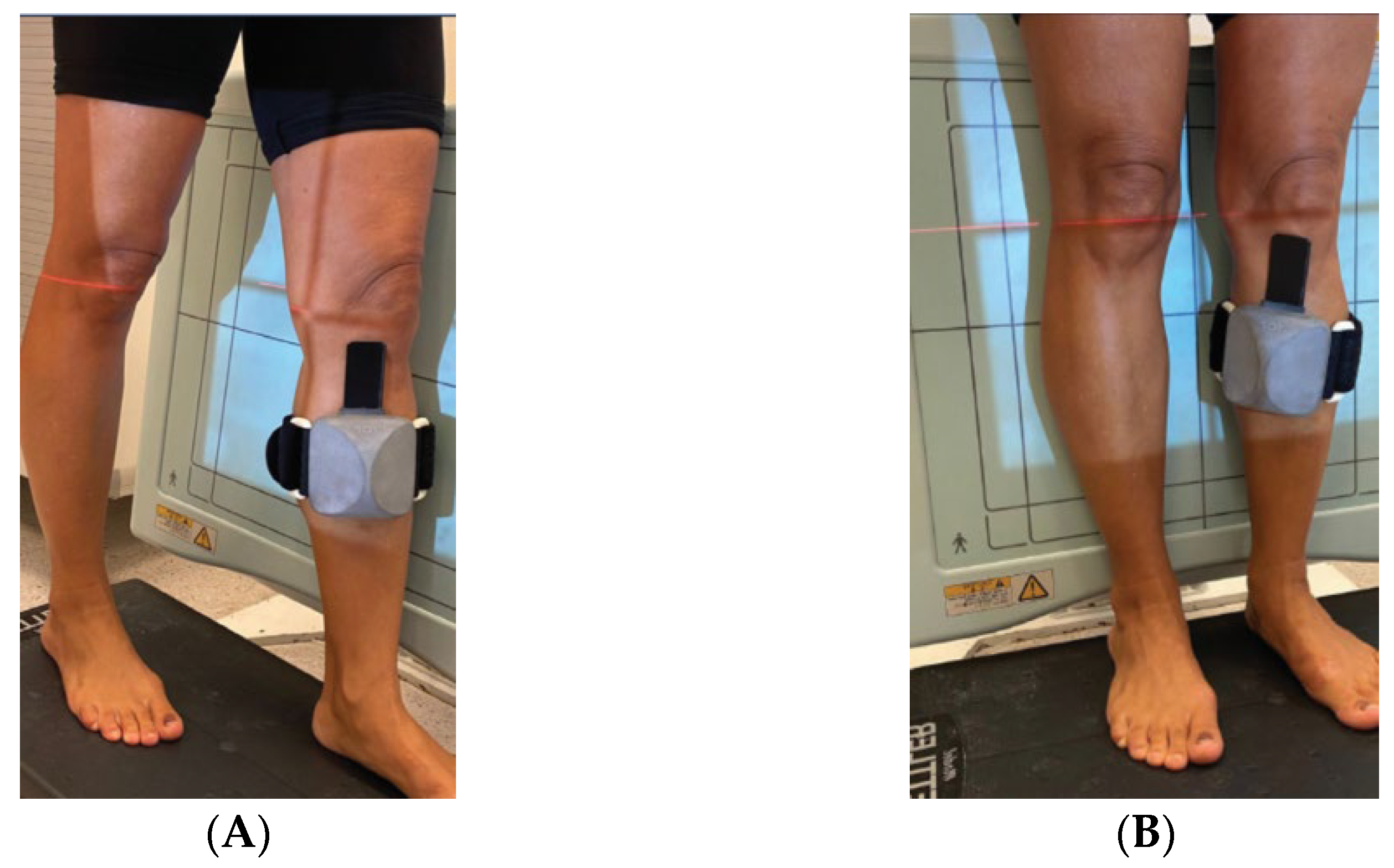
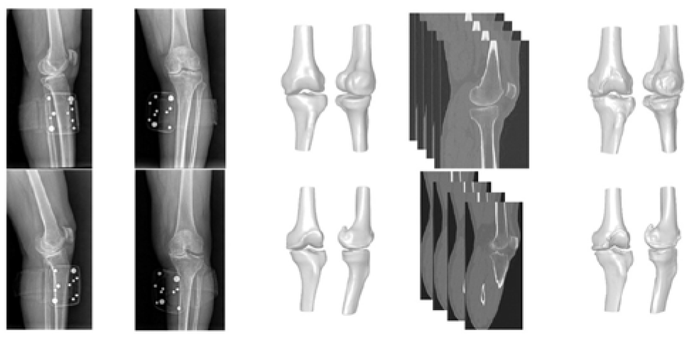
2. Materials and Methods
- = predicted surface point;
- = actual surface point;
- = # of points (For X-ray-based models.)
Statistical Analysis
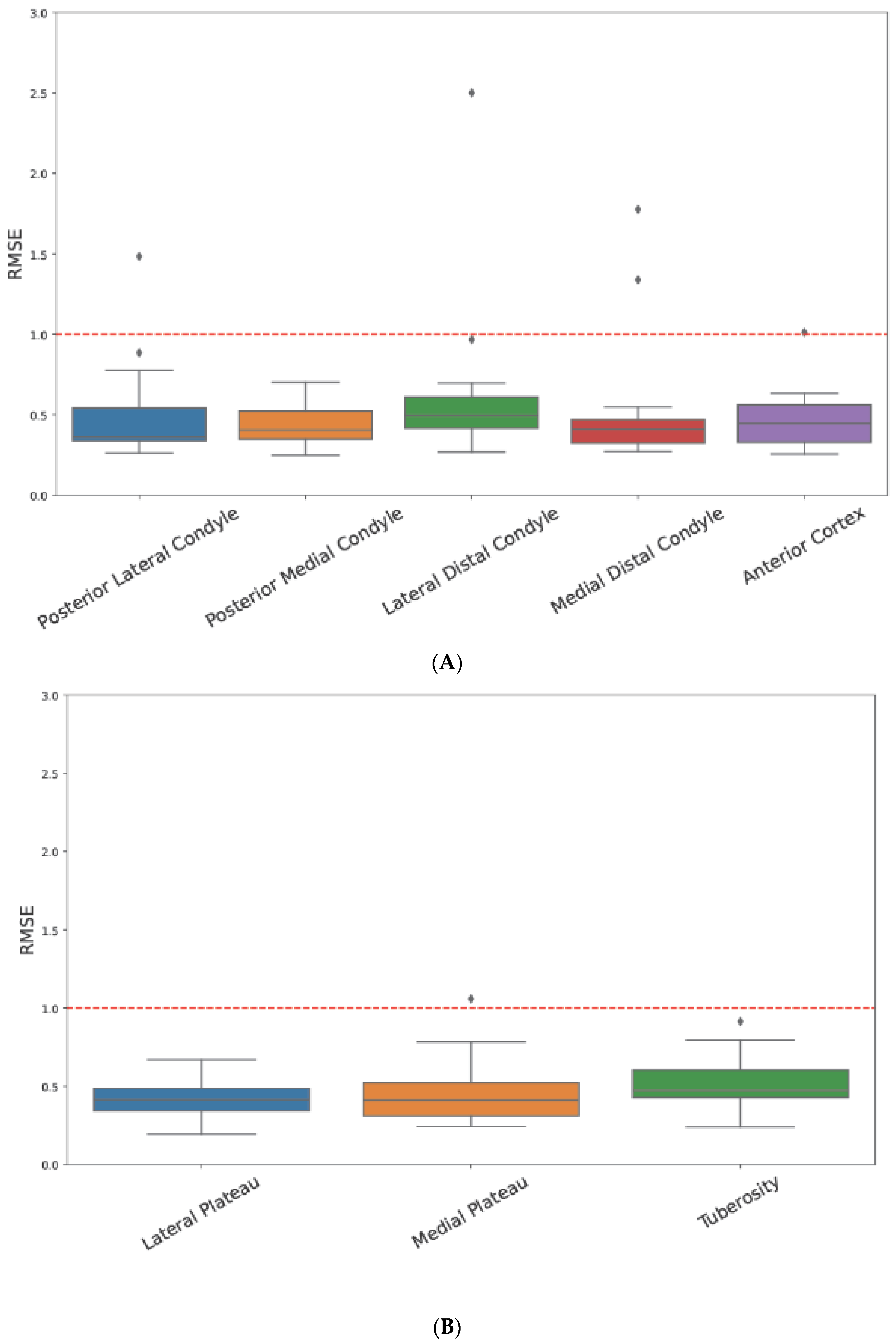
3. Results
4. Discussion
5. Conclusions
Author Contributions
Funding
Institutional Review Board Statement
Informed Consent Statement
Data Availability Statement
Conflicts of Interest
References
- Tanzer, M.; Makhdom, A.M. Preoperative Planning in Primary Total Knee Arthroplasty. J. Am. Acad. Orthop. Surg. 2016, 24, 220–230. [Google Scholar] [CrossRef] [PubMed]
- Kouyoumdjian, P.; Mansour, J.; Assi, C.; Caton, J.; Lustig, S.; Coulomb, R. Current concepts in robotic total hip arthroplasty. SICOT-J 2020, 6, 45. [Google Scholar] [CrossRef] [PubMed]
- Hsu, A.R.; Gross, C.E.; Bhatia, S.; Levine, B.R. Template-directed instrumentation in total knee arthroplasty: Cost savings analysis. Orthopedics 2012, 35, e1596–e1600. [Google Scholar] [CrossRef] [PubMed]
- Schotanus, M.G.M.; Schoenmakers, D.A.L.; Sollie, R.; Kort, N.P. Patient-specific instruments for total knee arthroplasty can accurately predict the component size as used peroperative. Knee Surg. Sports Traumatol. Arthrosc. 2017, 25, 3844–3848. [Google Scholar] [CrossRef] [PubMed]
- Mathis, D.T.; Hirschmann, M.T. Patient-specific instrumentation in total knee arthroplasty. Arthroskopie 2021, 34, 342–350. [Google Scholar] [CrossRef]
- Benignus, C.; Buschner, P.; Meier, M.K.; Wilken, F.; Rieger, J.; Beckmann, J. Patient Specific Instruments and Patient Individual Implants—A Narrative Review. J. Pers. Med. 2023, 13, 426. [Google Scholar] [CrossRef] [PubMed]
- Wang, J.; Wang, X.; Sun, B.; Yuan, L.; Zhang, K.; Yang, B. 3D-printed patient-specific instrumentation decreases the variability of patellar height in total knee arthroplasty. Front. Surg. 2023, 9, 954517. [Google Scholar] [CrossRef] [PubMed]
- Saffarini, M.; Hirschmann, M.T.; Bonnin, M. Personalisation and customisation in total knee arthroplasty: The paradox of custom knee implants. Knee Surg. Sports Traumatol. Arthrosc. 2023, 31, 1193–1195. [Google Scholar] [CrossRef] [PubMed]
- Fernandes, L.R.; Arce, C.; Martinho, G.; Campos, J.P.; Meneghini, R.M. Accuracy, Reliability, and Repeatability of a Novel Artificial Intelligence Algorithm Converting Two-Dimensional Radiographs to Three-Dimensional Bone Models for Total Knee Arthroplasty. J. Arthroplast. 2022, 38, 2032–2036. [Google Scholar] [CrossRef] [PubMed]
- Bhalodia, R.; Elhabian, S.Y.; Kavan, L.; Whitaker, R.T. DeepSSM: A Deep Learning Framework for Statistical Shape Modeling from Raw Images; Lecture Notes in Computer Science (including subseries Lecture Notes in Artificial Intelligence and Lecture Notes in Bioinformatics); Springer: Cham, Switzerland, 2018; Volume 11167. [Google Scholar]
- Heimann, T.; Meinzer, H.P. Statistical shape models for 3D medical image segmentation: A review. Med. Image Anal. 2009, 13, 543–563. [Google Scholar] [CrossRef]
- Cerveri, P.; Sacco, C.; Olgiati, G.; Manzotti, A.; Baroni, G. 2D/3D reconstruction of the distal femur using statistical shape models addressing personalized surgical instruments in knee arthroplasty: A feasibility analysis. Int. J. Med. Robot. Comput. Assist. Surg. 2017, 13, e1823. [Google Scholar] [CrossRef]
- Wysocki, M.A.; Lewis, S.A.; Doyle, S.T. Developing Patient-Specific Statistical Reconstructions of Healthy Anatomical Structures to Improve Patient Outcomes. Bioengineering 2023, 10, 123. [Google Scholar] [CrossRef]
- Sun, W.; Zhao, Y.; Liu, J.; Zheng, G. LatentPCN: Latent space-constrained point cloud network for reconstruction of 3D patient-specific bone surface models from calibrated biplanar X-ray images. Int. J. Comput. Assist. Radiol. Surg. 2023, 18, 989–999. [Google Scholar] [CrossRef] [PubMed]
- XPlan.ai. 3D Reconstruction from Standard 2D X-rays. Available online: https://www.xplan.ai/ (accessed on 23 December 2023).
- Zheng, G.; Hommel, H.; Akcoltekin, A.; Thelen, B.; Stifter, J.; Peersman, G. A novel technology for 3D knee prosthesis planning and treatment evaluation using 2D X-ray radiographs: A clinical evaluation. Int. J. Comput. Assist. Radiol. Surg. 2018, 13, 1151–1158. [Google Scholar] [CrossRef] [PubMed]
- Victor, J.; Van Doninck, D.; Labey, L.; Innocenti, B.; Parizel, P.M.; Bellemans, J. How precise can bony landmarks be determined on a CT scan of the knee? Knee 2009, 16, 358–365. [Google Scholar] [CrossRef] [PubMed]


| Bone | Landmark |
|---|---|
| Femur | Posterior Lateral Condyle |
| Posterior Medial Condyle | |
| Lateral Distal Condyle | |
| Medial Distal Condyle | |
| Anterior Cortex | |
| Tibia | Lateral Plateau |
| Medial Plateau | |
| Tuberosity |
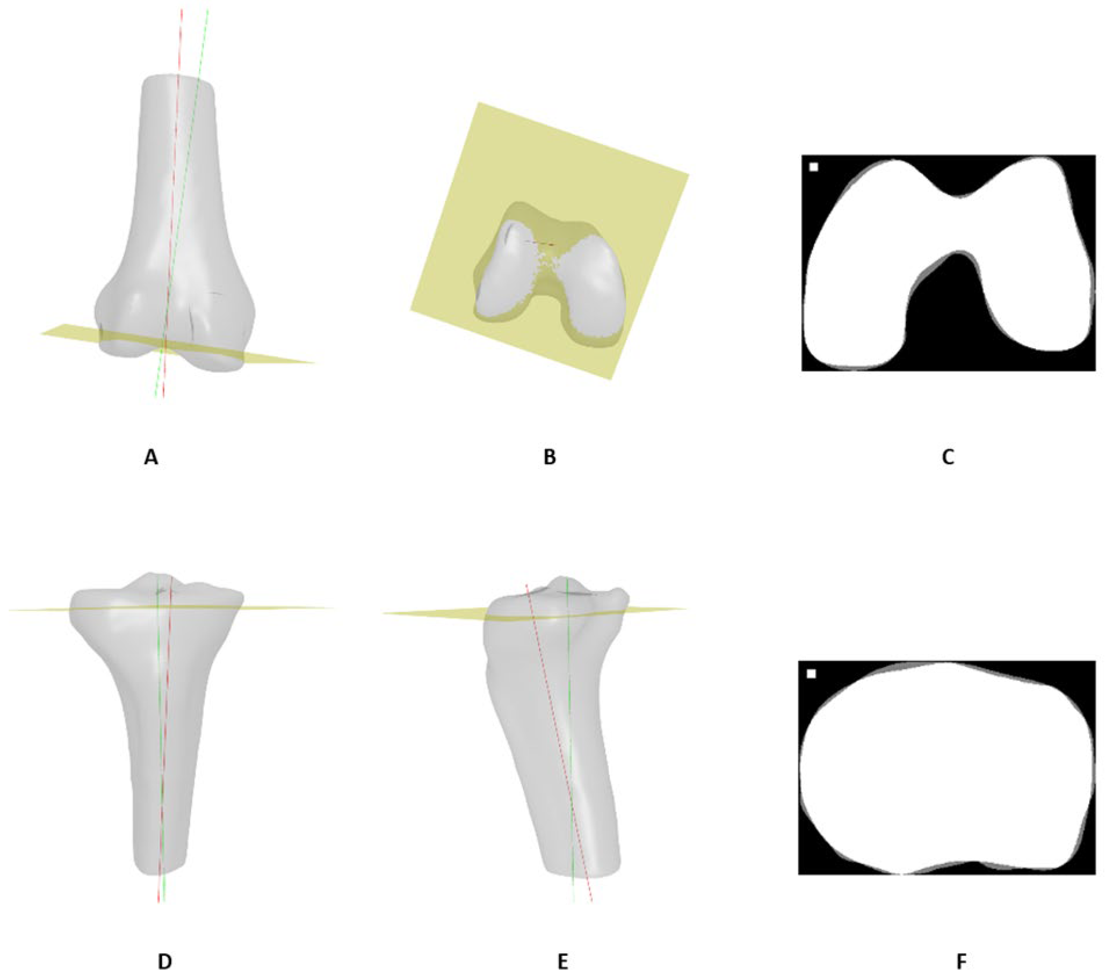
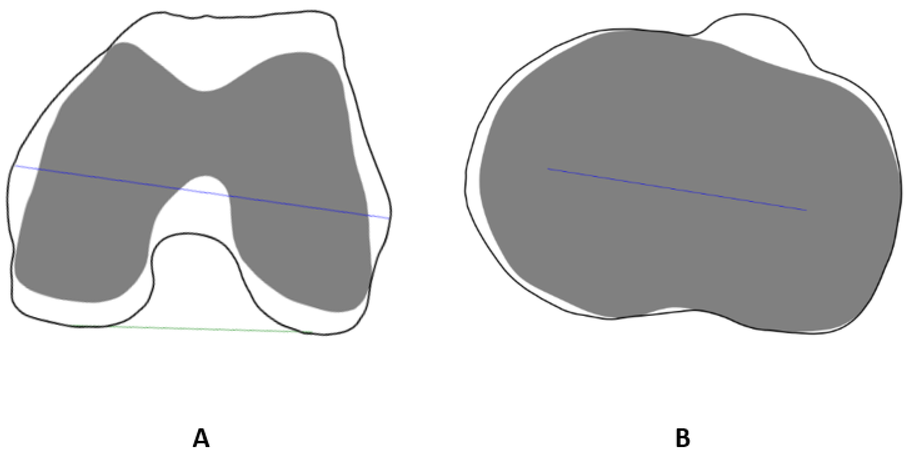
| Bone | Axis |
|---|---|
| Femur | Trans epicondylar axis (TEA) |
| Posterior condylar axis (PCA) | |
| Tibia | Medial–lateral transverse axis (MLTA) |
| Age (years) | 71 (±8.8) |
| Gender, Male (n, %) | 9 (50) |
| Height (m) | 1.67 (±0.41) |
| Weight (kg) | 86.9(±33.2) |
| BMI (kg/m2) | 30.7 (±10.7) |
| Side—affected knee | 11/7 (R/L) |
| Patient No. | Femur | Tibia |
|---|---|---|
| 1 | 0.57 | 0.74 |
| 2 | 0.97 | 0.94 |
| 3 | 0.82 | 0.81 |
| 4 | 0.77 | 1.03 |
| 5 | 0.90 | 0.97 |
| 6 | 1.04 | 0.79 |
| 7 | 0.72 | 0.70 |
| 8 | 1.21 | 0.98 |
| 9 | 1.03 | 1.09 |
| 10 | 1.57 | 1.09 |
| 11 | 1.41 | 0.90 |
| 12 | 0.75 | 0.84 |
| 13 | 0.85 | 0.93 |
| 14 | 0.87 | 0.88 |
| 15 | 0.97 | 0.99 |
| 16 | 0.72 | 0.86 |
| 17 | 0.74 | 0.69 |
| 18 | 0.87 | 0.62 |
| Mean ± SD | 0.93 ± 0.25 | 0.88 ± 0.14 |
| Human-Level Baseline (between-Measurement Angular Deviations, CT vs. CT) | CT vs. X-Ray Angular Deviation (between-Measurement Angular Deviations, CT vs. X-ray) | |
|---|---|---|
| TEA | 1.43° (±1.16°) | 1.89° (±1.52°) |
| PCA | 1.71° (±1.48°) | 1.78° (±1.49°) |
| MLTA | 2.56° (±1.82°) | 2.82° (±2.18°) |
Disclaimer/Publisher’s Note: The statements, opinions and data contained in all publications are solely those of the individual author(s) and contributor(s) and not of MDPI and/or the editor(s). MDPI and/or the editor(s) disclaim responsibility for any injury to people or property resulting from any ideas, methods, instructions or products referred to in the content. |
© 2024 by the authors. Licensee MDPI, Basel, Switzerland. This article is an open access article distributed under the terms and conditions of the Creative Commons Attribution (CC BY) license (https://creativecommons.org/licenses/by/4.0/).
Share and Cite
Factor, S.; Gurel, R.; Dan, D.; Benkovich, G.; Sagi, A.; Abialevich, A.; Benkovich, V. Validating a Novel 2D to 3D Knee Reconstruction Method on Preoperative Total Knee Arthroplasty Patient Anatomies. J. Clin. Med. 2024, 13, 1255. https://doi.org/10.3390/jcm13051255
Factor S, Gurel R, Dan D, Benkovich G, Sagi A, Abialevich A, Benkovich V. Validating a Novel 2D to 3D Knee Reconstruction Method on Preoperative Total Knee Arthroplasty Patient Anatomies. Journal of Clinical Medicine. 2024; 13(5):1255. https://doi.org/10.3390/jcm13051255
Chicago/Turabian StyleFactor, Shai, Ron Gurel, Dor Dan, Guy Benkovich, Amit Sagi, Artsiom Abialevich, and Vadim Benkovich. 2024. "Validating a Novel 2D to 3D Knee Reconstruction Method on Preoperative Total Knee Arthroplasty Patient Anatomies" Journal of Clinical Medicine 13, no. 5: 1255. https://doi.org/10.3390/jcm13051255
APA StyleFactor, S., Gurel, R., Dan, D., Benkovich, G., Sagi, A., Abialevich, A., & Benkovich, V. (2024). Validating a Novel 2D to 3D Knee Reconstruction Method on Preoperative Total Knee Arthroplasty Patient Anatomies. Journal of Clinical Medicine, 13(5), 1255. https://doi.org/10.3390/jcm13051255