Rainfall Spatial-Temporal Variability and Trends in the Thamirabharani River Basin, India: Implications for Agricultural Planning and Water Management

Abstract

Rainfall is critical to agricultural and drinking water supply in the Thamirabharani river basin. The upper catchment areas of the Thamirabharani basin are located in high-elevated forest regions, and rainfall variability affects dam inflow and outflow. The well-known methods for rainfall analysis such as the coefficient of variation (CV), the precipitation concentration index (PCI), and trend analysis by Mann-Kendall and Sen’s slope test, as well as the Sen’s graphical innovative trend method (ITA) recently reported in several studies, were used. Rainfall data from gauge stations and the satellite-gridded Multisource Weighted Ensemble Precipitation (MSWEP) dataset were chosen for analysis at the annual and four-season time scales, namely, the Southwest Monsoon, Northeast Monsoon, winter, and summer seasons from 1991 to 2020. The mean annual PCI value reflects irregular monthly rainfall distribution (PCI > 20) in all gauge stations. The spatial monthly rainfall distribution of PCI values remarkedly shows a moderate distribution in the western and an anomalous distribution in the eastern part of the basin. The annual mean rainfall ranges from 718.4 to 2268.6 mm/year, decreasing from the high altitude zone in the west to the low plains and coastal regions in the east. Seasonal rainfall contributes about 42% from the NEM, 30.6% from the SWM, 22.8% from summer, and 3.9% from winter, with moderate variability (CV less than 30%). Ground stations experienced extremely high interannual variability in rainfall (more than 60%). Trend analysis by the MK, TFPW-MK, and ITA methods shows increasing annual rainfall in the plains and coastal regions of the basin; particularly, more variations among the seasons were observed in the Lower Thamirabharani sub-basin. The NEM and summer season rainfall are statistically significant and contribute to the increasing trend in annual rainfall. The ITA method performed better in the annual and seasonal scale for detecting the rainfall trend than the MK and TFPW-MK test. The Lower Thamirabharani sub-basin in the eastern part of the basin receives more rain during the NEM than in other areas. To summarize, the low plains in the central and coastal regions in the southeast part experience an increase in rainfall with irregular monthly distribution. This study helps farmers, governments, and policymakers in effective agricultural crop planning and water management.

1. Introduction

Rainfall is a pivotal component of the hydrological cycle, and variations in its pattern have a direct impact on the water supply [1]. Climate change influences rainfall characteristics such as quantity, intensity, and seasonality, as well as the occurrence of drought and flood. Extreme rainfall events affect the seasonal or annual amount of precipitation [2]. Lack of rainfall lowers reservoir water levels, decreases moisture content, reduces streamflow, and causes a depletion of the groundwater table [3]. Changes in rainfall quantity and frequency have a direct impact on stream flow pattern and demand, spatiotemporal allocation of run-off [4], groundwater reserves [5,6], and soil moisture [7]. Understanding these changes has far-reaching implications for water resources, the environment, terrestrial ecosystems, the ocean, biodiversity, agriculture, and food security [8].

Drought and floodlike hazards are frequently caused by extreme fluctuations in rainfall patterns. Drought is characterized by reduced or inadequate rainfall, which restricts plant development and eventually affects yields. Flooding is caused by a heavy downpour of rainfall, which deteriorates crop growth [9,10]. The impact of climatic extremes varies throughout geographical features and time, depending on agricultural practices, agroecology, and a farmer’s ability to adapt to those conditions [11]. Changes in rainfall patterns also play a role in the emergence of new crop pests and diseases [12,13].

Rainfall has a significant role in determining water availability in an area. Analyzing precipitation characteristics and patterns is a critical task for improving water resource utilization and for practitioners engaged in water resource planning and making policy decisions [14,15]. The Intergovernmental Panel on Climate Change report (2008) also emphasized the growing importance of trend analysis in meteorological and hydrological data for detecting major changes induced by climate change [16]. A dense network of meteorological stations is required for effectively defining the spatial trends of climatic variables. In remote areas, owing to limited spatial coverage of meteorological stations, satellite-based gridded products are used as an input for trend identification, modelling, statistical analysis, and other climatological applications [17]. Several research works on gridded data have been conducted comparing and assessing the correlation between satellite-derived and observed data [18,19,20]. Gridded satellite data were validated and applied in trend and variability analyses across many river basins [21,22,23,24]. Extensive studies have been carried out for various places throughout the world, examining the pattern, trends, and distribution of rain using station and satellite-gridded datasets [25,26,27,28].

Many methodologies in the parametric [29,30] and nonparametric tests [31,32] have been reported for assessing trends using gridded rainfall datasets. Among them, the Sen’s slope estimation [33] and the Mann-Kendall (MK) test are the most often used nonparametric method for detecting trends in time series data [34,35,36,37,38,39,40]. Recently, an innovative trend analysis (ITA), a graphical method, was widely used, and it does not need any assumptions in time series data [5,25,33,35,41]. These nonparametric methods have several advantages, such as managing missing data and not requiring any assumptions [42,43]. The main drawback of these methods is the effect of autocorrelation on time series data, and to reduce this effect, many modifications have been proposed in the MK test [44,45,46]. Studies in analyzing precipitation trends have been reported across the world in various river basins such as the Indus basin [47], Vea catchment [48], Awash River basin [49], and Yarlung river basin [40]. Similarly, in India, trend studies using gridded satellite products have been performed in the Kosi River basin [50], the Cauvery basin [51,52,53], and the Gomati basin [54].

The Thamirabharani River originates in the Western Ghats; it is a perennial river that serves as a major source of water for agricultural and municipal needs in the southern districts of the Tamil Nadu [55]. The majority of the basin’s upstream area and reservoirs are at high altitude and close to the Western Ghats. Rainfall variability caused by global warming affects inflow, outflow, and water discharge in the dam [56], reducing agricultural production and negatively impacting areas that rely on dam water. Therefore, studying climate variability and trends may help the agriculture sector and government in effective water management planning. In a few studies, only rainfall trends were examined in the Thamirabharani basin [57] and the Lower Thamirabharani sub-basin [58] while no spatial scale study has been conducted in the basin. In the Thamirabharani basin, the distribution of gauge stations is quite sparse and also no rainfall stations have been located in the high elevated areas where the majority of the reservoirs are located, making it difficult to detect trends in isolated places. Hence, the current study was carried out to examine the spatial trend pattern and variability in rainfall over the Thamirabharani river basin using both gauge stations and satellite-gridded rainfall data and then to apply this information for appropriate agricultural planning.

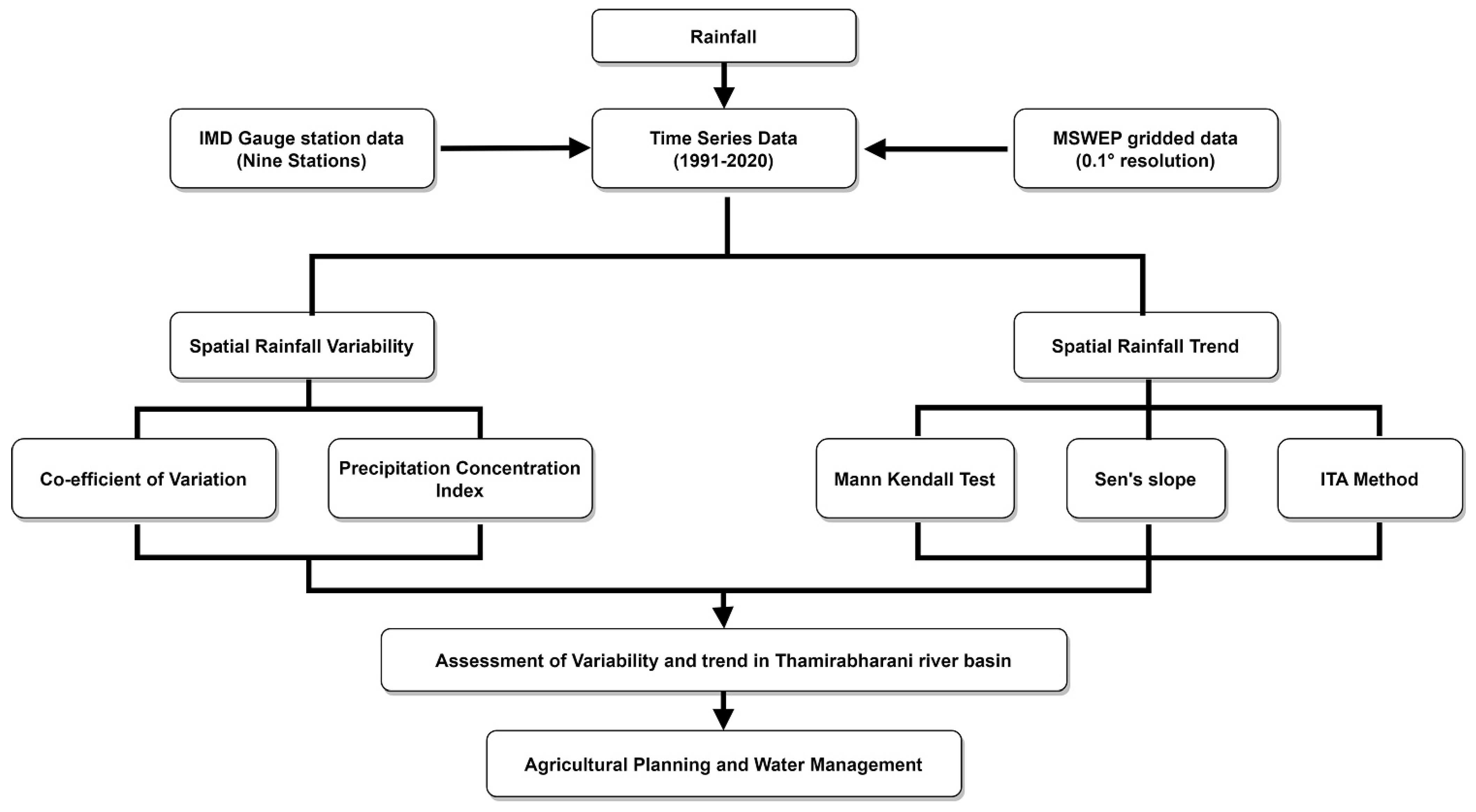
2. Materials and Methods

Overall methodology is represented as a flowchart in Figure 1 and the same is explained elaborately in the following subsections.

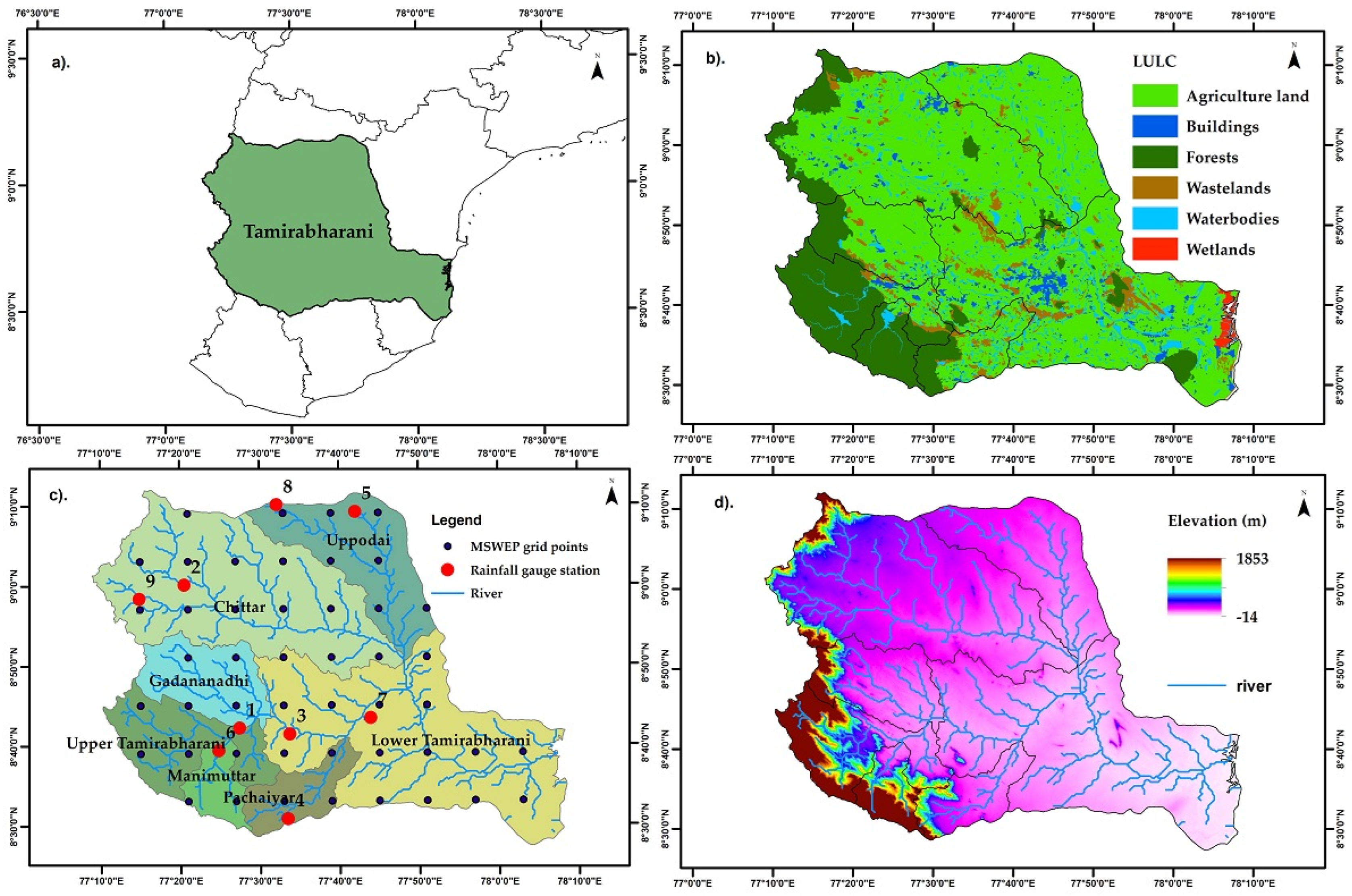
The Thamirabharani, a perennial river, originates from the Pothigai hills (Agastyarkoodam Peak) in the Western Ghats of Southern India. The entire river basin covers an area of approximately 5717.08 km² and is located in the Tenkasi, Tirunelveli, and Thoothukudi districts of Tamil Nadu. The river flows through 11 anicuts spread over three districts, with a total distance of 125 km [55]. The entire basin is divided into seven sub-basins, with catchment areas found in Chittar, Gadananadhi, Manimuthar, Pachiyar, and Upper Thamirabharani, and some parts of Chittar, Lower Thamirabharani, and the Uppodai sub-basin located largely in low stream areas (Figure 2). The basin area comprises three forms of natural features: dense forest in the high-altitude region, gentle agricultural areas, and low-lying coastal areas in the east [59]. The general climatic pattern of the basin is subtropical type with an annual mean temperature ranging from 23 to 27 °C. The entire basin receives an average rainfall of 985.77 mm per year. Agriculture in this region depends on water released from dams, and the main crops cultivated include rice, sugarcane, bananas, groundnuts, and floriculture. The major crop-growing seasons are the Kharif and rabi season, which coincide with two monsoon rainfalls [60].

2.1. Data Used

Ground level observed gauge station data was obtained from the India Meteorological Department (IMD). Data quality checking and validation were performed using the procedure described in [61]. After quality assessment, only 9 stations with no missing data were chosen for research out of 15 gauge stations. For this study, rainfall data from the years 1991 to 2020 was used, and it was classified as annually, Southwest Monsoon (SWM) (June–September), Northeast Monsoon (NEM) or postmonsoon season (October–December), winter season (January–February), and summer season or premonsoon season (March–May) [62]. The descriptive statistics of rainfall at nine gauge stations that include standard deviation, skewness, and kurtosis are presented in

Table 1. Descriptive statistics of annual and seasonal rainfall (mm) at study sites of the Thamirabharani river basin.

Stations	Annual			SWM			NEM			Summer			Winter
	SD	SK	KT	SD	SK	KT	SD	SK	KT	SD	SK	KT	SD	SK	KT
Ambasamuthiram	281.4	−0.4	0.4	248.9	0.1	−0.4	91.1	0.9	−0.1	112.1	1.2	1.5	52.8	0.5	−0.7
Ayikudi	304.3	1.2	2.7	238.2	1.2	2.3	73.2	−0.2	−1.4	101.1	0.6	−0.3	48.4	2.1	4.8
Cheranmahadevi	278.3	0.2	−0.5	216.4	0.1	−1.1	56.7	1.3	2.1	109.7	2.1	5.9	46.9	1.8	4.2
Kalugumalai	391.0	−0.4	0.2	256.2	−0.1	0.0	76.0	0.0	−0.9	121.3	0.3	−0.7	95.8	1.8	2.5
Kalakadu	268.8	0.1	−0.5	219.7	0.7	0.6	84.5	1.2	1.6	77.2	1.4	2.2	35.7	1.4	2.0
Manimuthar	400.8	−0.5	0.3	337.5	−0.4	−0.8	82.3	0.4	−0.9	136.1	1.5	2.2	78.6	0.8	0.1
Palayamkottai	238.3	0.1	−0.3	198.1	0.3	−0.6	56.7	0.5	−0.1	80.0	0.5	0.2	59.1	2.2	5.2
Sankarankovil	304.8	0.5	0.3	253.6	1.1	1.7	62.6	0.9	1.2	85.4	0.8	0.3	44.4	2.5	7.2
Shenkottai	620.2	0.2	0.2	371.4	1.4	4.3	268.3	0.9	0.4	209.7	1.3	1.4	121.9	1.9	3.2

SD—Standard deviation, SK—Skewness, KT—Kurtosis.

. This indicates that mean rainfall of the annual and seasonal period exhibits both negative and positive values in skewness and kurtosis. Figure 1 illustrates the location, Land-use and land cover, geographical location of rainfall gauge station, and elevation profile of the Thamirabharani river basin, whereas

Table 2. Details of rainfall gauge stations located in the Thamirabharani river basin.

Station No.	Station Name	Latitude (°N)	Longitude (°E)	Elevation (m)	Sub-Basin
1	Ambasamuthiram	8.70	77.46	67	Upper Thamirabharani
2	Ayikudi	9.00	77.34	167	Chittar
3	Cheranmahadevi	8.69	77.56	62	Lower Thamirabharani
4	Kalakadu	8.51	77.56	127	Pachiyar
5	Kalugumalai	9.15	77.71	119	Uppodai
6	Manimuthar	8.66	77.41	85	Manimuthar
7	Palayamkottai	8.72	77.73	43	Lower Thamirabharani
8	Sankarankovil	9.17	77.54	157	Uppodai
9	Shengottai	8.97	77.25	179	Chittar

presents the details of the rainfall gauge stations.

The recently released Multisource Weighted Ensemble Precipitation (MSWEP) dataset with a 0.1° resolution was derived by merging gauge data, satellite, and reanalysis data and used for spatial analysis. This dataset includes bias-corrected climate mean data from the Climate Hazards Group Precipitation Climatology (CH-Pclim), stream flow data from the USGS Geospatial Attributes, PRISM climatic precipitation data, and global runoff data from the Global Runoff Data Centre (GRDC). Additionally, it includes various gridded satellite-based precipitation products, including TMPA 3B42RT, PERSIANN, CHIRPS, CMORPH, SM2RAIN-ASCAT, and GSMaPMV, as well as reanalysis datasets such as ERA-Interim, NCEP-CFSR, JRA-55, and many others [63]. The methodology, accuracy, and quality assessment of the MSWEP product can be seen in [64]. In India, MSWEP data are compared and validated with IMD data [65,66] and used in rainfall analysis [21,27,32]. The statistical comparison of MSWEP-gridded data shows a relative absolute error of less than 1, indicating a good relation with gauge station data (

Table A1. Comparative statistics of ground station and satellite-gridded data.

Statistics\Station	Ambasamuthiram	Ayikudi	Cheranmahadevi	Kalakadu	Kalugumalai	Manimuthar	Palayamkottai	Sankarankovil	Shengottai
Annual
MAE	80.7	95.6	69.4	64.6	104.4	253.2	124.0	150.4	248.1
RAE	0.6	0.5	0.3	0.5	0.6	0.8	0.7	0.8	0.6
MBE	−54.4	−95.6	−52.0	27.7	−83.8	−28.6	−59.4	−138.5	60.2
PBE	−5.3	−11.1	−6.5	3.1	−11.7	−2.6	−7.7	−17.6	4.0
NSE	0.6	0.8	0.9	0.7	0.6	0.3	0.5	0.4	0.6
SWM
MAE	29.4	70.1	26.5	36.1	45.7	53.6	38.1	35.3	49.4
RAE	0.4	0.5	0.3	0.5	0.4	0.5	0.4	0.5	0.5
MBE	13.9	−6.5	9.1	5.9	−2.8	−15.4	7.0	−13.9	−4.6
PBE	3.1	−1.5	2.2	1.5	−0.6	−3.8	1.8	−3.7	−0.9
NSE	0.9	0.6	0.9	0.8	0.9	0.8	0.9	0.8	0.9
NEM
MAE	17.8	9.7	7.9	13.8	11.4	11.8	14.6	11.6	30.3
RAE	0.2	0.2	0.2	0.2	0.2	0.2	0.3	0.2	0.2
MBE	−5.6	−7.6	−5.0	−5.0	−9.8	−9.6	−4.8	−9.7	−17.4
PBE	−4.6	−6.4	−5.7	−3.9	−8.2	−6.8	−5.1	−11.4	−4.3
NSE	0.9	1.0	1.0	0.9	1.0	1.0	0.8	0.9	1.0
Winter
MAE	14.8	11.4	9.2	25.1	16.6	14.3	10.6	8.4	22.1
RAE	0.4	0.6	0.4	0.5	0.7	0.5	0.5	0.5	0.6
MBE	9.5	−2.5	6.4	6.3	−4.7	11.3	3.7	−1.1	5.8
PBE	14.3	−6.9	13.7	8.9	−11.9	20.6	9.4	−3.1	10.8
NSE	0.7	0.6	0.9	0.6	0.1	0.8	0.7	0.8	0.5
Summer
MAE	17.3	24.4	54.4	23.2	24.4	33.4	14.4	14.1	29.7
RAE	0.2	0.4	1.0	0.5	0.5	0.4	0.3	0.3	0.3
MBE	−4.3	−21.8	−29.1	13.0	−19.1	−10.3	−8.1	−5.0	9.1
PBE	−2.8	−12.5	−17.2	6.9	−16.3	−5.0	−5.2	−2.5	3.7
NSE	1.0	0.8	0.4	0.8	0.8	0.8	0.9	0.9	0.9

MAE—mean absolute error, RAE—relative absolute error, MBE—mean bias error, PBE—percentage bias error, NSE—Nash–Sutcliffe model efficiency.

). These gridded data were analyzed and interpolated in ArcGIS 10.5 using the IDW and Kriging approach [67].

2.2. Rainfall Analysis

Variability in rainfall was analyzed using Coefficient of variation (CV) and Precipitation Concentration Index (PCI).

2.2.1. Coefficient of Variation (CV)

To assess the variability of the rainfall in the study area, the coefficient of variation (CV) was used (see [68] for more details). The level of variability depends on the indicator; thus, it follows that the higher the CV value, the higher the variability in rainfall and vice versa. It is expressed in percentage (%).

The value of CV was obtained by the above-described method and was used to categorize the degree of variability of rainfall events as low variability (CV < 20%), moderate variability (20 < CV < 30%), high variability (CV > 30%), very high variability (CV > 40%), and extremely high interannual variability of rainfall (CV > 70%) [69].

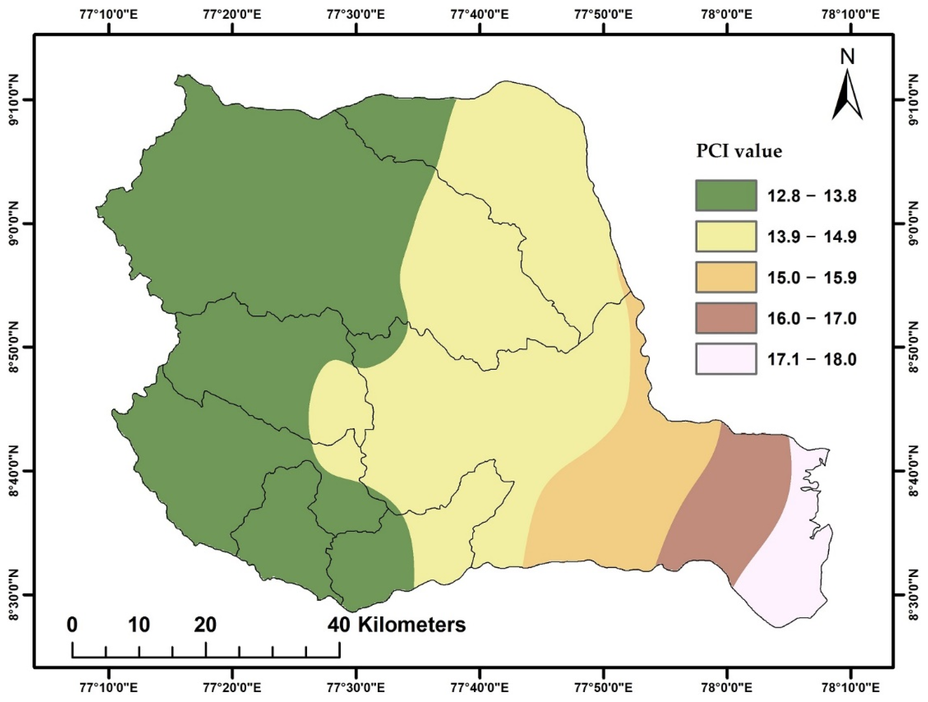
2.2.2. Precipitation Concentration Index (PCI)

The PCI is a monthly rainfall distribution index derived from time series data that can be used to assess the seasonality of rainfall. It is calculated using the method described by Oliver [70], and PCI values less than 10 indicate a consistent precipitation distribution, values 11 to 15 indicate a moderate precipitation concentration, and values 16 to 20 indicate an anomalous precipitation distribution. PCI values greater than 20 dramatically indicate an irregular precipitation distribution. PCI is calculated by the given equation

$$PCI=\frac{{\displaystyle {\sum }_{i=1}^{12}{P}_i{}^2}}{{({\displaystyle {\sum }_{i=1}^{12}{P}_i})}^2}$$

(1)

where P_i is the quantity of rainfall on ith month, used to calculate annual PCI values.

2.3. Rainfall Trend Analysis

The trend in time series rainfall data was analyzed using the methods: i. Mann-Kendall test, ii. Sen’s slope estimator, iii. trend-free prewhitening Mann-Kendall test, and iv. innovative trend analysis (graphical method).

The Mann-Kendall (MK) trend test is a nonparametric, rank-based method for detecting significant monotonic trends in meteorological and hydrological data [71,72]. It has the advantage of not requiring any prerequisite conditions for the time series data to be normally distributed or the presence of a linear line or missing data values, etc. [73]. To determine whether there is a uniform linear growth or fall tendency in the trend analysis, the MK test was first applied. Then, the linear trend was evaluated using the nonparametric Sen’s slope estimate, which provides a statistical (mm/year) representation of the increase or decrease in the rainfall under consideration [74].

Historically, linear regression was the most commonly used method for trend identification, but it is parametric and needs data to be normally distributed. The MK test has been widely used in trend analysis due to its simplicity, flexibility to accept missing and non-normal data distributions, and ability to mitigate the impact of outliers and remove major data imperfections [75]. Additionally, the MK test can be used for different time periods, including monthly, seasonal, and yearly.

$$S={\displaystyle \sum _{i=1}^{n-1}{\displaystyle \sum _{j=i+1}^n\mathrm{sgn}(x_j-x_i)}}$$

(2)

where

$$\mathrm{sgn}(x_j-x_i)=\{\begin{array}{ccc}1& if& (x_j-x_i) > 0\\ 0& if& (x_j-x_i)=0\\ -1& if& (x_j-x_i) < 0\end{array}$$

(3)

In which x_j and x_i are the rainfall observations recorded at times j and i (with j > i), respectively, and n is the length of the time series data. Under the null hypothesis (H₀) condition, the distribution of S is symmetrical and normal in the limit as n becomes large, with zero mean and variance:

$$Var (S)=\left[n(n-1) (2n+5) - {\displaystyle \sum _{i=1}^m{t}_i(t_i-1)(2t_i+5)}\right]/18$$

(4)

where t_i indicates the number of ties with extend i.

Finally, the statistic (Z_mk) for the given variance (S) is calculated by Equation (5)

$$Z_{mk}=\{\begin{array}{ccc}\frac{S-1}{\sqrt{Var(S)}}& for \mathrm{S} > 0& \\ 0& for \mathrm{S}=0& \\ \frac{S+1}{\sqrt{Var(S)}}& for \mathrm{S} < 0& \end{array}$$

(5)

The positive (or negative) of Z_mk from Equation (5) indicates the increasing (or decreasing) direction of the trend in the time series. In this study, data were employed for trend analysis at a 95% significance level and the null hypothesis for no trend in rainfall was rejected if Z_mk was greater than 1.96.

2.3.1. Sen’s Slope Estimator

Sen’s slope estimation is a nonparametric method for calculating the magnitude of the trend in meteorological/hydrological time series data. It was computed using the method outlined by Sen [73]. In a given time series data, a positive coefficient indicates an upward trend and vice versa.

The magnitude of the trend for a given time series, viz., x₁, x₂, x₃,…, x_n rainfall data at time t₁, t₂, t₃, …, t_n (t₁ < t₂ < t₃ < … < t_n), for each N pairs of rainfall observations x_j and x_i taken at times t_j and t_i, the gradient (Q_k) can be calculated by the equation given below:

$$Q_k=\frac{x_j-x_i}{t_j-t_i} \mathrm{for} \mathrm{k}=1, 2,\mathrm{\dots }, \mathrm{N}$$

(6)

With 1 < i < j < n and t_j > t_i. The trend estimates in the time series data x_1, x_2, x_3,…, x_n can be calculated as the median Q_med of the N values of Q_k, ranked from the smallest to the largest.

$${\mathrm{Q}}_{med}=\{\begin{array}{cc}{Q}_{\frac{(N+1)}{2}}& if \mathrm{N} \mathrm{is} \mathrm{odd}\\ \frac{Q_{[N/2]}+Q_{[(N+2)/2]}}{2}& if \mathrm{N} \mathrm{is} \mathrm{even}\end{array}$$

(7)

The positive (or negative) value of Q_med represents the increasing (or declining) trend and the zero value represents no trend in rainfall data.

2.3.2. Trend Free Prewhitening (TFPW)-Mann-Kendall Test

In order to eliminate the presence of serial correlation in time series rainfall data, prewhitening of the data is important [76]. When the time series data are not random and influenced by autocorrelation, the trend factor is eliminated from the data and prewhitened before the trend test is applied [77]. The linear trend component of the original time series data is removed and prewhitened using the lag-1 serial correlation coefficient. Finally, the prewhitened data is used to find the trend through the Mann-Kendall trend test [78].

2.3.3. Innovative Trend Analysis (ITA)

The innovative trend analysis (ITA) method is a graphical trend analysis method that does not require any assumptions such as serial correlation, sample or population size, non-normality, and so on, which are required by traditional trend analysis methods (Mann-Kendall test, Spearman’s rho tests, cumulative sum, and so on). Trend graphs were generated using the method adopted and the procedures followed as per [33,41].

First, the time series is separated into two equal parts that are then sorted in ascending order individually. The first and second halves of the time series are then plotted on the X- and Y-axes, respectively. There is no trend in the time series if the data are accumulated on the 1:1 ideal line (45° line). If the data are in the top triangular section of the 1:1 ideal line, there is an increasing tendency in the time series. When data are gathered in the bottom triangular area of the 1:1 line, the time series shows a falling trend. The trend slope (TS) and significance were calculated as represented in [79]. In this study, the ITA method was applied at 95% significance levels in time series rainfall data.

3. Results

3.1. Mean Rainfall Distribution and Variability over the Thamirabharani River Basin

The Thamirabharani river basin has two monsoon seasons: SWM and NEM. The average annual and seasonal rainfall received at nine locations is given in

Table 3. Mean rainfall (mm) over the Thamirabharani basin during the annual and seasonal period.

Station	Annual	SWM	NEM	Winter	Summer
Ambasamuthiram	1039.2	121.2	692.4	66.7	158.9
Ayikudi	744.6	118.5	429.7	37.3	159.1
Cheranmahadevi	797.3	86.8	514.4	45.2	151.0
Kalakadu	969.8	125.1	560.1	80.1	204.5
Kalugumalai	666.1	115.7	420.3	34.9	95.1
Manimuthar	1119.2	138.7	739.3	87.9	153.3
Palayamkottai	759.0	94.8	481.4	46.4	136.4
Sankarankovil	666.3	80.8	406.8	31.0	147.7
Shenkottai	1465.3	430.8	664.1	84.5	285.9
Mean	914.1	145.8	545.4	57.1	165.8

. The annual mean rainfall received across the nine stations ranged from 666.1 to 1465.3 mm/year, with maximum rainfall in Shengottai followed by Manimuthar (1119.2 mm/year) and Ambasamuthiram (1039.2 mm/year), respectively. Shengottai received higher mean seasonal rainfall during the SWM (430.5 mm) and summer (285.9 mm), but Manimuthar received more rainfall during the NEM (739.3 mm) and winter (87.9 mm), respectively. Figure 3 depicts the spatial distribution of mean annual rainfall over the basin, which ranges from 718.4 to 2268.6 mm. The highest mean annual rainfall (more than 2000 mm) was recorded in regions of the Gadananadhi, Upper Thamirabharani, and Manimuthar sub-basins located in the basin’s western region, as well as in higher elevation areas. However, the Thamirabharani basin’s low stream command regions (the eastern part of the basin) received the least rainfall (less than 1000 mm).

Figure 4 represents the spatial distribution of mean seasonal rainfall in the SWM (152.6 to 964.0 mm), the NEM (377.7 to 727.5 mm), summer (119.8 to 436.8 mm), and winter (29.7 to 63.8 mm). Because of the cyclonic activity and nearness to the Indian Ocean, certain areas of the Lower Thamirabharani sub-basin (especially the eastern part) receive more rainfall (approximately more than 400 mm) during the NEM season than the central part of the basin (Figure 4b). The regions in the southwestern section of the basin (upstream regions) receive more seasonal and annual rainfall than those in the east due to higher elevation, extensive forest cover, being near the Western Ghats, and receiving bimodal rainfall.

The coefficient of variation (CV) calculated for each station at yearly and seasonal time intervals is shown in

Table 4. The coefficient of variation (%) in rainfall over the Thamirabharani basin during the annual and seasonal period.

Station	Annual	SWM	NEM	Winter	Summer
Ambasamuthiram	27.1	75.2	35.9	79.2	70.6
Ayikudi	40.9	61.8	55.4	130.0	63.6
Cheranmahadevi	34.9	65.4	42.1	103.7	72.7
Kalakadu	40.3	60.7	45.7	119.6	59.3
Kalugumalai	40.4	73.0	52.3	102.3	81.2
Manimuthar	35.8	59.4	45.7	89.5	88.8
Palayamkottai	31.4	59.8	41.2	127.4	58.7
Sankarankovil	45.7	79.3	62.3	143.3	57.8
Shenkottai	42.3	62.3	55.9	144.3	73.3

. The CV for annual mean rainfall ranges from 27.1 to 45.9%, indicating moderate to extremely high variability in rainfall distribution across all locations. The seasonal rainfall variability ranged from 35.9% in the NEM (Ambasamuthiram) to 143.3% in the winter season (Shengottai). This conclusion agrees with the findings of Malarvizhi [57], who reported increasing variability in rainfall over the Thamirabharani river basin in both annual and seasonal periods.

In Figure 5, the MSWEP data reveals that the mean annual variability in rainfall is low (12.8 to 20.1%), whereas rainfall variability is moderate to high during the SWM and NEM seasons. Winter has very high to extremely high interannual variability compared to the summer CV, which shows moderate to very high variability (greater than 60% CV). Throughout the year, the eastern portions of the basin, especially in the Lower Thamirabharani sub-basin, experience higher variability than other areas. Some parts of the Manimuthar and Upper Thamirabharani sub-basin (high elevation areas) have larger variability throughout the NEM and winter seasons (the red-colored region in Figure 5).

3.2. Precipitation Concentration Index (PCI) over the Thamirabharani River Basin

Figure 6 shows a heat map of the yearly PCI value calculated from 30 years (1991–2020) of monthly rainfall data. Annual PCI values ranged from 11.8 to 42.3, indicating a moderate to irregular monthly rainfall distribution across the basin. Except for Shengottai, all other stations experienced a greater number of erratic monthly rainfall distribution. Shengottai station (17.7) has the lowest mean PCI value during the 30 years, followed by Ayikudi (21.5) and Manimuthar (21.7), both of which are located in the vicinity of the Western Ghats. Sankarankovil, Palayamkottai, and Cheranmahadevi stations have the highest mean PCI values (PCI greater than 23) and are located in the low-plain areas of the basin. The reason could be the NEM season, which is largely governed by the cyclonic activity in the Bay of Bengal of the Indian Ocean [80].

Figure 7 depicts the number of years of the precipitation concentration distribution. Over the study period, most years with an irregular monthly distribution (PCI > 20) of rainfall were seen with an average of 19 years. Shengottai and Ayikudi stations had the maximum number of years with an anomalous precipitation distribution (approximately more than 15 years), this could be because these two stations are located in the western part of the basin, near a narrow pass in the Western Ghats, and receive rain from both monsoons. From Figure 6, it is also observed that there is a greater number of years with irregular monthly rainfall distribution, followed by an anomalous precipitation concentration.

Figure 8 represents the spatial distribution of the mean PCI values over 30 years (1991–2020) using MSWEP-gridded data. Annual PCI values ranged from 12.9 to 18.2, reflecting that the Thamirabharani river basin had a consistent to moderate monthly rainfall distribution. In comparison to the eastern low plain region, the majority of the western part of the river basin experiences a moderate monthly rainfall distribution, but the southeastern part of the basin has an anomalous precipitation distribution. This indicates the rainfall distribution is moderate in the western regions of the basin, where these regions located on the leeward side of the Western Ghats may receive rainfall from both monsoons. The anomalous precipitation in the low plain areas of the southeast part of the basin, mainly due to NEM, depends on cyclone intensity in the Bay of Bengal.

3.3. Mann-Kendall Trend in Rainfall over the Thamirabharani River Basin

The results of increasing and decreasing trends by MK and TFPWT-MK tests in rainfall over the Thamirabharani River Basin are summarized in

Table A2. Trend statistics over the Thamirabharani river basin.

Station No.		Ambasamuthiram	Ayikudi	Cheranmahadevi	Kalakadu	Kalugumalai	Manimuthar	Palayamkottai	Sankarankovil	Shengottai
Annual
MK	Zmk	−0.9	1.3	−0.5	1.1	−1.6	−0.8	−1.3	−0.3	0.9
	SS	−5.8	6.0	−3.0	9.3	−19.5	−6.1	−7.6	−0.9	5.0
TFPWMK	Z	−0.9	1.7	−0.9	−0.9	−1.0	1.4	−0.8	0.4	−1.7
	SS	−6.7	8.5	−4.7	−9.6	−6.2	10.3	−3.0	3.3	−21.6
SWM
MK	Zmk	0.7	0.5	−0.2	0.0	0.1	0.5	0.7	0.3	0.9
	SS	0.3	0.6	−0.2	0.03	0.7	0.8	1.0	0.5	0.8
TFPWMK	Z	0.7	1.7	0.6	1.6	0.3	0.6	0.6	0.7	0.4
	SS	1.6	2.6	0.4	2.4	0.5	1.0	0.9	1.0	1.8
NEM
MK	Zmk	−0.6	0.8	−0.5	0.9	−1.6	−1.3	−0.8	0.5	0.5
	SS	−3.6	3.9	−2.9	9.6	−11.9	−6.1	−3.0	2.1	2.0
TFPWMK	Z	−1.2	1.3	−0.8	−0.6	−1.5	0.6	−0.1	0.2	−2.1
	SS	−6.8	5.8	−3.4	−3.8	−7.6	4.8	−0.5	1.2	−13.6
Winter
MK	Zmk	−0.3	−0.4	−1.1	0.0	−1.7	0.6	−0.7	−1.8	−0.6
	SS	−0.3	−0.04	−0.8	−0.01	−2.4	0.5	−0.4	−1.3	−0.1
TFPWMK	Z	−0.3	0.1	−1.1	−0.1	0.6	0.3	−1.6	−0.8	−1.4
	SS	−0.3	0.0	−0.9	−0.1	0.6	0.3	−0.8	−0.4	−1.3
Summer
MK	Zmk	−1.3	1.9	−0.2	−0.5	−0.3	0.5	−1.2	−0.04	1.9
	SS	−2.5	4.6	−0.3	−0.9	−1.7	1.7	−1.6	−0.1	2.8
TFPWMK	Z	−1.0	2.1	−0.2	−1.3	0.1	−0.4	−0.5	1.5	−0.5
	SS	−1.9	4.3	−0.5	−1.3	0.5	−0.8	−0.5	2.5	−2.9

MK—Mann-Kendal test, TFPWMK—trend-free prewhitening Mann-Kendall test, Z—Z value, SS—Sen’s slope (mm). Bold text—represents significant at 95% significance level.

. The annual rainfall did not show any significant trends in both tests. A nonsignificant decreasing trend (p > 0.05) in annual rainfall was observed at Ambasamuthiram, Cheranmahadevi, Kalakadu, Kalugumalai, and Palayamkottai locations. During the SWM, all stations show a nonsignificant positive trend in MK and TFPWT-MK tests, except Cheranmahadevi, which shows a negative in the MK test. Rainfall in Shengottai was found to be significantly lower (−13.6 mm/year) than in other locations during the NEM. Summer rainfall increased significantly at Ayikudi in both tests and Shengottai in the MK test. Though station data does not show any significant trends, however, the TFPW-MK method detected some trends after applying prewhitening. This finding is consistent with [57], who stated that stations in the western part of the basin had a significantly increasing trend over the summer.

Figure 9 shows the spatial variation of annual and seasonal rainfall trends from 1991 to 2020, based on MSWEP data. Figure 9a depicts that annual precipitation is increasing across the whole basin, and this trend is statistically significant in the low plain region only. The annual increase in rainfall ranges from 5.2 to 9.6 mm. However, the high-elevation region in the basin’s southwestern part (part of the Manimuthar and Upper Thamirabharani sub-basins) shows a nonsignificant increase in annual rainfall, ranging from 9.7 to 14.4 mm/year. SWM rainfall shows a nonsignificant (Z_mk < 1.96) declining trend in the southeastern part, more reduction in the Lower Thamirabharani sub-basin regions, and an increase in the regions of the west part (Figure 9b). This supports the trend of decreasing SWM rainfall reported by Isabella et al. [58]. Figure 9c shows a significant (Z > 1.96) increase in rainfall during the NEM in the eastern part of the basin, especially in the Lower Thamirabharani sub-basin region. The eastern region of the basin exhibits a greater increase throughout the NEM season (more than 4.3 mm/year), while the western part has a nonsignificant decrease in rainfall, which may be related to cyclonic activity during the NEM season. Rainfall in winter does not show any significant trends over the entire basin (Figure 9d). The rainfall trend pattern in the summer season shows a significant (Z_mk > 1.96) increase in the western part of the basin. The quantity of rainfall detected using the Sen’s slope method shows an increase in rainfall in part of the Chittar, Gadananadhi, Upper Thamirabharani, and Manimuthar sub-basins, ranging between 2.2 and 7 mm/year (Figure 9e). These regions are mostly high-elevated and densely forested areas, and these forests act as a moisture regime for summer rainfall [52]. Additionally, a nonsignificant increase in the part of the Lower Thamirabharani sub-basin areas (low plain area) was observed.

The trend-free prewhitening Mann-Kendall (TFPW-MK) method is used to remove series correlation in rainfall data, and Figure 10 illustrates the spatial pattern of the trend observed during the annual and seasonal periods. Both this methodology and the one that was previously explained showed similar trends. Rainfall increased during the annual, NEM, and summer but non significantly decreased during the SWM and winter (Figure 10b,d). However, the number of significant points was reduced after prewhitening the rainfall data. Annual rainfall indicated a pattern of increase from 5.8 to 12.2 mm/year over the basin (Figure 9a), 4.2 to 6.9 mm/year during the NEM season (Figure 10c), and 3.2 to 6.1 mm/year during the winter season (Figure 10e). A similar pattern of trend in the MK test and the TFPW-MK test was found; however, significant points reduced in the TFPW-MK test imply that the presence of serial correlation was removed. Additionally, the increase in rainfall quantity was found to be higher in the TFPW-MK compared to the MK test.

3.4. Innovative Trend Analysis over the Thamirabharani River Basin

The slope of the innovative trend observed over the Thamirabharani river basin based on the analysis of the study period (1991–2020) is portrayed in

Table A3. Statistics of trend analysis by ITA method in Thamirabharani river basin.

Stations	Annual		SWM		NEM		Winter		Summer
	TS	TY	TS	TY	TS	TY	TS	TY	TS	TY
Ambasamuthiram	−1.53	NM	−0.39	NM	−0.65	NM	−0.34	NM	−0.15	NM
Ayikudi	12.71	MT	2.81	NM	8.37	MT	−0.94	NM	2.48	NM
Cheranmahadevi	5.67	NM	−0.40	NM	3.90	NM	−1.31	NM	3.49	NM
Kalakadu	−0.12	NM	1.02	NM	−0.37	NM	−0.42	NM	−0.35	NM
Kalugumalai	6.12	NM	1.89	NM	1.34	NM	−1.26	NM	4.15	MT
Manimuthar	24.11	MT	0.44	NM	17.91	NM	1.78	NM	3.98	NM
Palayamkottai	1.36	NM	0.14	NM	3.92	NM	−2.70	MT	0.01	NM
Sankarankovil	8.67	MT	1.42	MT	2.55	NM	−1.07	MT	5.56	MT
Shengottai	−12.22	NM	5.10	NM	−7.72	NM	−5.17	MT	−4.43	NM

TS—trend slope (mm), TY—trend type, NM—Nonmonotonic, MT—monotonic trend. Bold text indicates significance at a 95% level.

. The trend slope of mean annual rainfall is dominated by positive values (increasing trend). From the above table, an increasing slope of trend for Ayikudi (12.71 mm/year), Cheranmahadevi (5.67 mm/year), Manimuthar (24.11 mm/year), Sankarankovil (8.67 mm/year), and Kalugumalai (6.12 mm/year) was observed. Meanwhile, decreasing trends in Shenkottai (−12.22 mm/year), Ambasamuthiram (−1.53 mm/year), and Kalakadu (−0.12 mm/year) were noted. Rainfall at the Cheranmahadevi station increased significantly (at p = 0.05), while it dropped at the Shengottai station. The decreasing trend was observed more at the Shengottai station, which is located upstream and near the Western Ghats. It was observed that three of the nine stations only exhibit monotone trends.

Figure S1 also shows ITA graphs for the annual mean rainfall. Except for two stations (Ambasamuthiram and Cheranmahadevi), the rest of the stations in the SWM season exhibited increasing rainfall trend, but it was more in Shengottai (5.10 mm/year) and Ayikudi (2.81 mm/year). Except in the SWM season, Shengottai showed a decrease in rainfall on an annual and seasonal scale. The related ITA graphs for the four seasons are given in Figures S2–S5. The seasonal analysis of rainfall showed that most of the stations observed positive values, except in the winter, where negative values (decreasing trend) dominated the most. Overall, the annual and seasonal trend analysis of station data revealed varied rainfall trends. Furthermore, when compared with MK trend analysis, the ITA method detected more significant trends [35].

Figure 11 illustrates the spatial pattern of the trend slope during annual and seasonal mean rainfall as determined using the ITA method. The positive trend slope values range from 5.3 to 14.3 mm/year, with the highest increase (more than 9 mm/year) seen in the western part of the basin, especially in the Upper Thamirabharani, Manimuthar, and Gadananadhi sub-basins (Figure 11a). More than 90% of the grid points showed an upward trend at a 95% significant level. On a seasonal scale, except during the NEM season, the increased rainfall trend was more in the western part of the basin compared to the eastern low stream areas (Figure 11b–e). The Lower Thamirabharani sub-basin received more rainfall throughout the NEM season than other places. During the SWM, rainfall decreased in the eastern half of the basin (Figure 11b), and the percentage of significant points was lower (around 40 per cent). Comparing the ITA technique and MK trend test, the identified trend pattern was similar in annual and seasonal rainfall across the Thamirabharani river basin.

3.5. Comparison Results of Trend Analysis Methods

The percentage of significant gridded points identified by the Mann-Kendall, trend-free prewhitening-Mann-Kendall, and innovative trend analysis methods is shown in Figure 12. In the annual and seasonal periods, the ITA approach found more significant points than other methods. According to the MK test, the percentage of significant points in the annual, the NEM, and summer season were 79, 39, and 33%, respectively, while they were reduced in the TFPW-MK test. Both methods did not find any significant trends in the SWM and winter. In the ITA method, the corresponding significant points were 100, 35, 91, 78, and 100% for the annual, the SWM, the NEM, winter, and summer, respectively. This finding is similar to the report by [29,45], in which the ITA method identified a trend that was not detected by the MK test.

4. Discussion

Rainfall has both direct and indirect impacts on agricultural production. It is a critical element in deciding crop type, cropping pattern, and yields in rainfed areas. Water released from reservoirs is primarily responsible for agriculture and drinking water supply in the Thamirabharani river basin [55]. Hence, characterizing the trend and variability of rainfall is important for sustainable crop planning and water management strategies [81,82]. Previous studies in the same basin [57] and in the Lower Thamirabharani sub-basin [58] used only station data and did not examine spatial pattern. Recently, ITA has been used in many studies due to its advantages over other trend analysis methodologies [35]. From the highlighted gaps in the expertise, the current study was conducted to determine rainfall variability and trend using gauge station and satellite-gridded data.

The annual mean rainfall in gauge stations ranged from 666.1 to 1465.3 mm/year, with an overall average of 914.1 mm/year. Considering the seasonal average, the NEM got 545.4 mm of rain, followed by summer (165.8 mm) and the SWM (145.8 mm). NEM rainfall makes the most significant contribution (more than 59 per cent), followed by summer rainfall (18.1%), and SWM (16%). This is supported by a similar report by [57,83] in the Thamirabharani river basin and also in the Vellar basin [84] and Lower Bhavani basin [85] of Tamil Nadu, where NEM contributed major rainfall to the basin. NEM rainfall is ideal for agricultural activity throughout the rabi season. 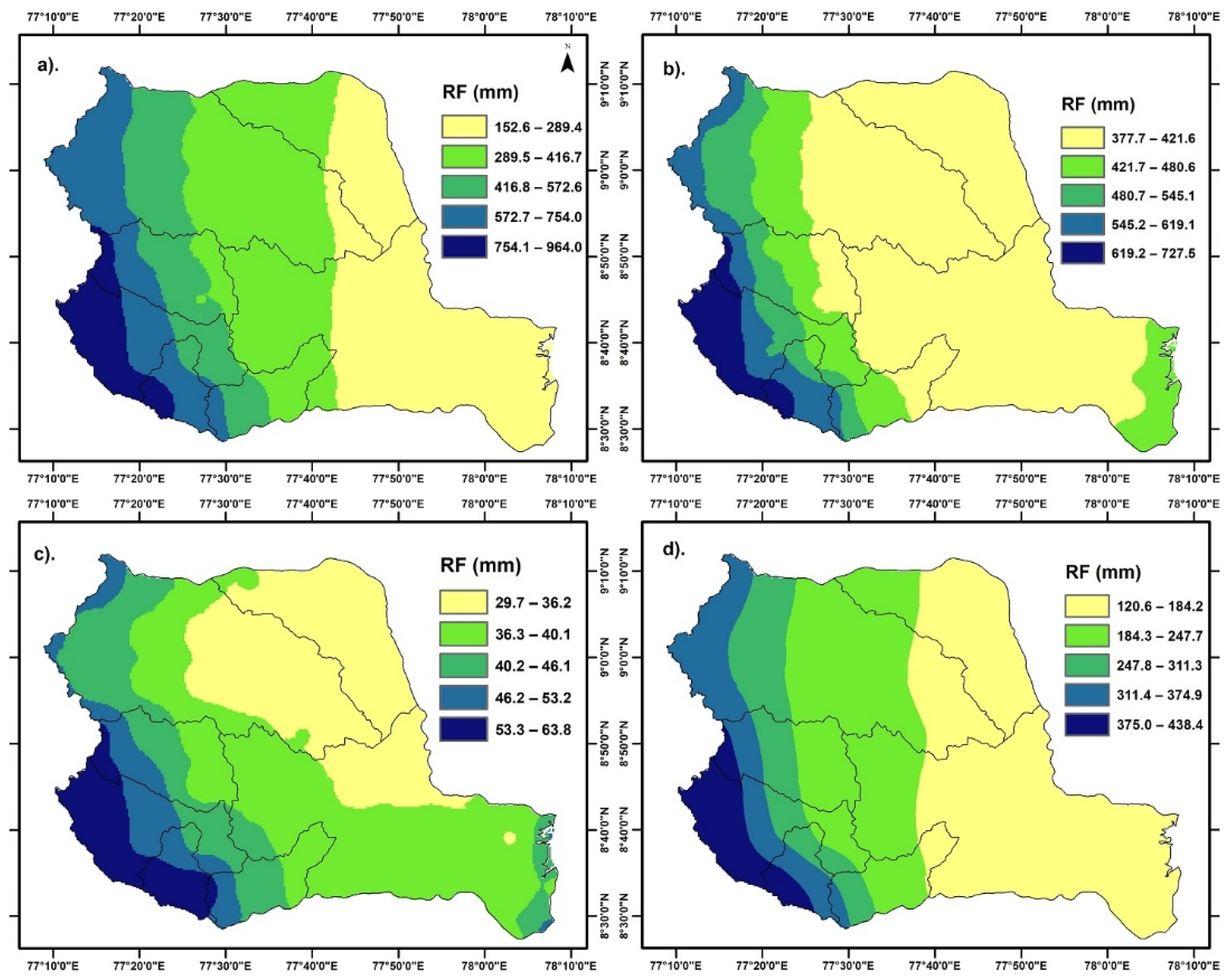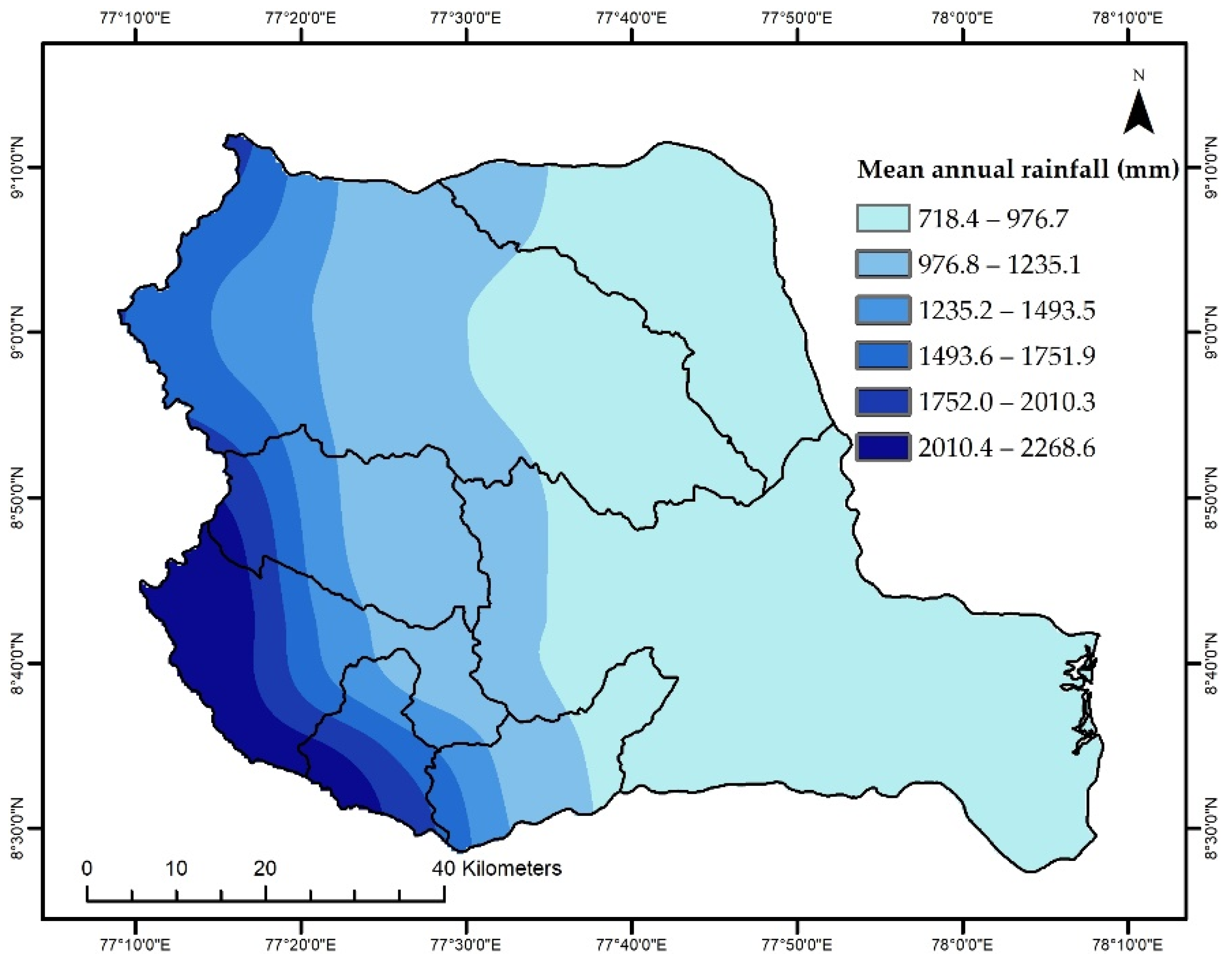Summer rainfall determines premonsoon crop planning for the Kharif season; however, later crop cultivation and production are dependent on rainfall from the SWM in the Thamirabharani river basin [86,87]. The spatial pattern of mean annual rainfall spans from 744.36 to 2189.47 mm/year, with rainfall increasing from the low plains to the high-elevation zones in the western region. MSWEP data showed more rainfall than ground data, it has been observed that the catchments (highly elevated areas) receive more rainfall (Figure 3), which might increase dam inflow and outflow and these regions that are located on the western side of the basin have largely deep forests and receive rainfall throughout the year [88].

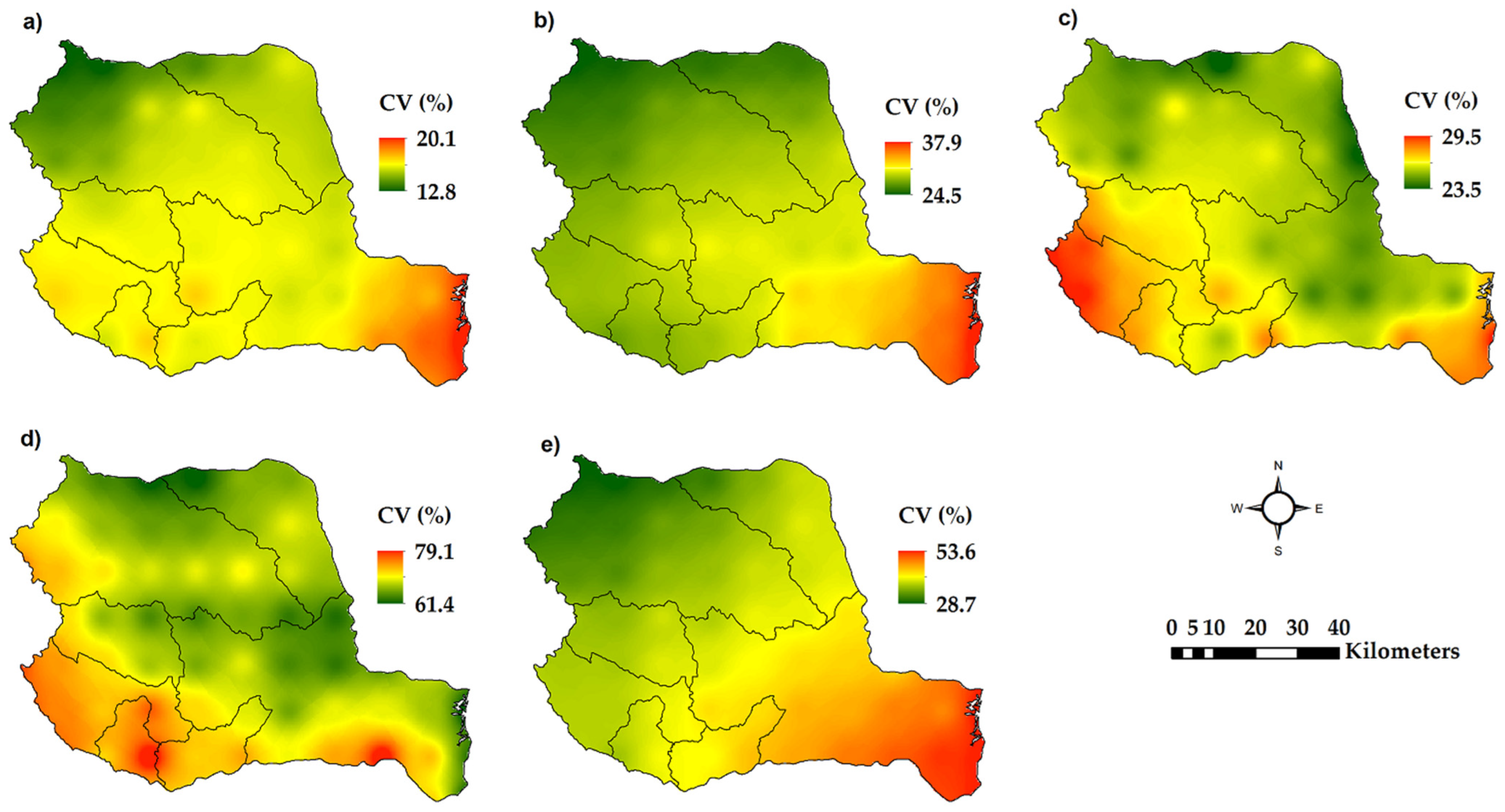
Variability in annual mean rainfall exhibits very high variability (CV greater than 40%) in all stations, except Ambasamuthiram (Table 3), which could have an impact on the agricultural activity in the basin. A similar result was reported in the Thamirabharani basin [57]. Seasonal rainfall in all stations experiences very high interannual variability (on average, more than 60% CV). Spatial variation of the CV on annual rainfall is low (12.8 to 20.1%) while seasonal rainfall has moderate to extremely high interannual variability. A similar report by [88] also mentioned high to very high interannual variability of rainfall in the Western Ghats, which could be attributed to moisture supply by the lower tropospheric winds that govern rainfall activity over the Western Ghats [89]. Low-lying coastal areas in the southeast part experience higher variability in annual and seasonal rainfall than other regions of the basin (Figure 5). The spatial scale assessment aids in a better understanding of rainfall variability and its impacts on water availability [46]. It is also necessary at the basin level for environmental impact studies, crop planning, and watershed management planning [29,45]. In rainfed agriculture, the seasonal unpredictability of rainfall has a substantial impact on crop productivity [90,91,92]. 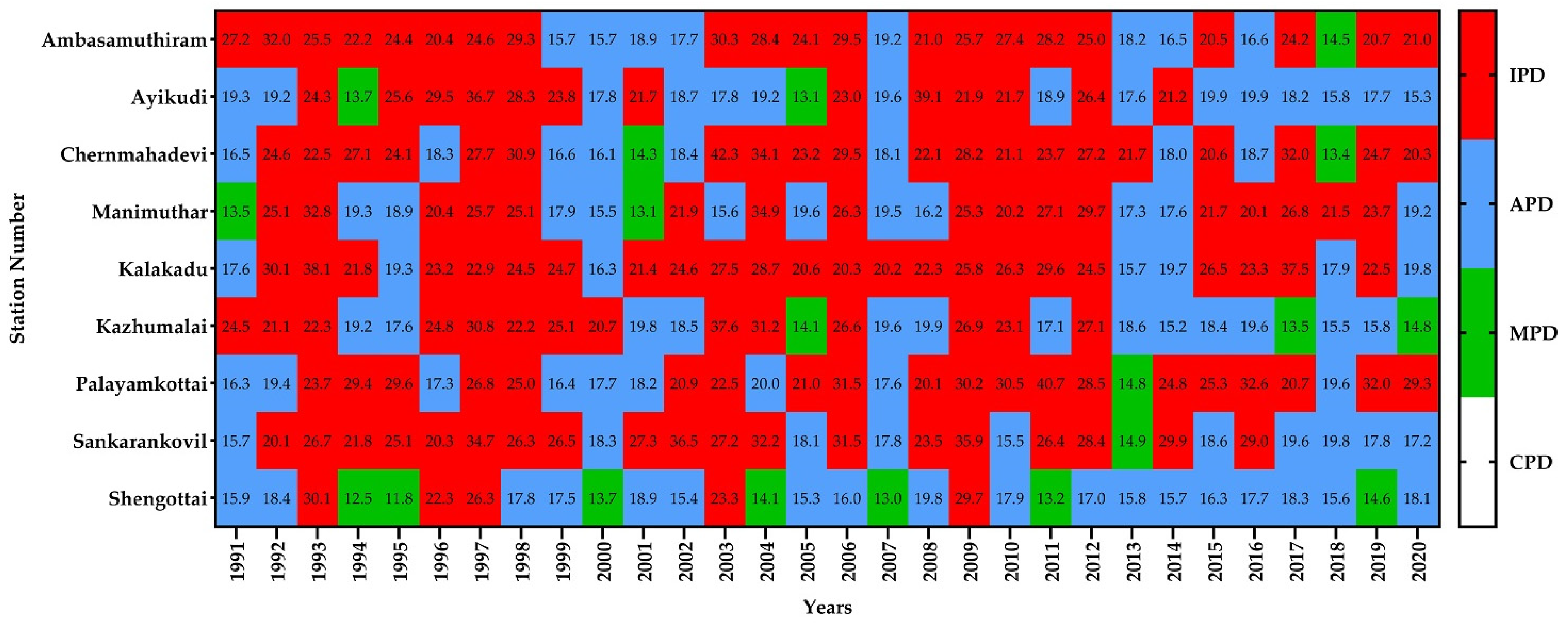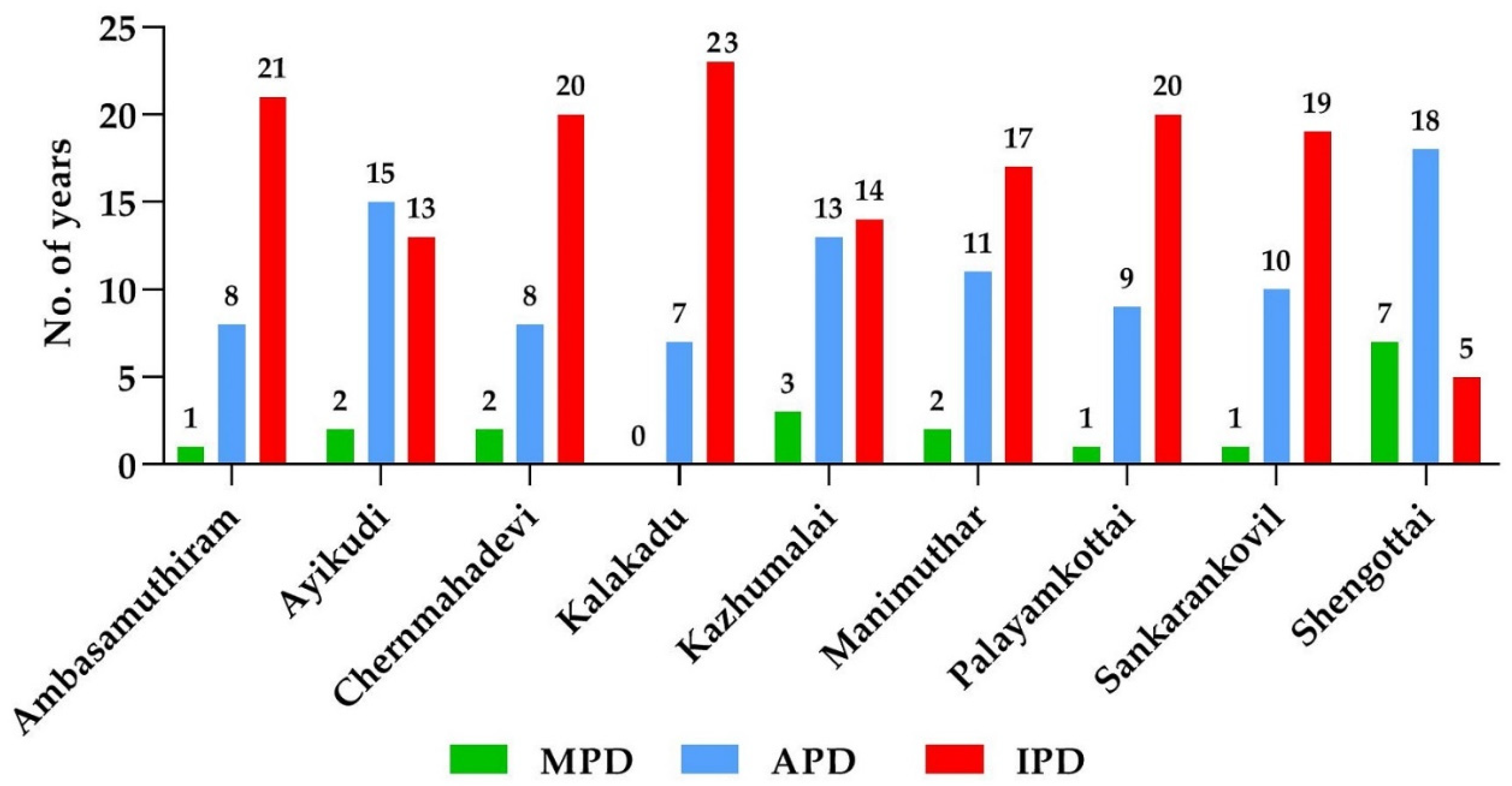PCI values show moderate to irregular monthly distribution of rainfall, whereas satellite data indicates a moderate distribution in the western half (Figure 8) and an anomalous to irregular pattern of precipitation distribution in low plain and low-lying coastal areas of the basin. The precipitation concentration index is crucial for integrated water resource management, drought and flood risk identification, and environmental conservation [93].

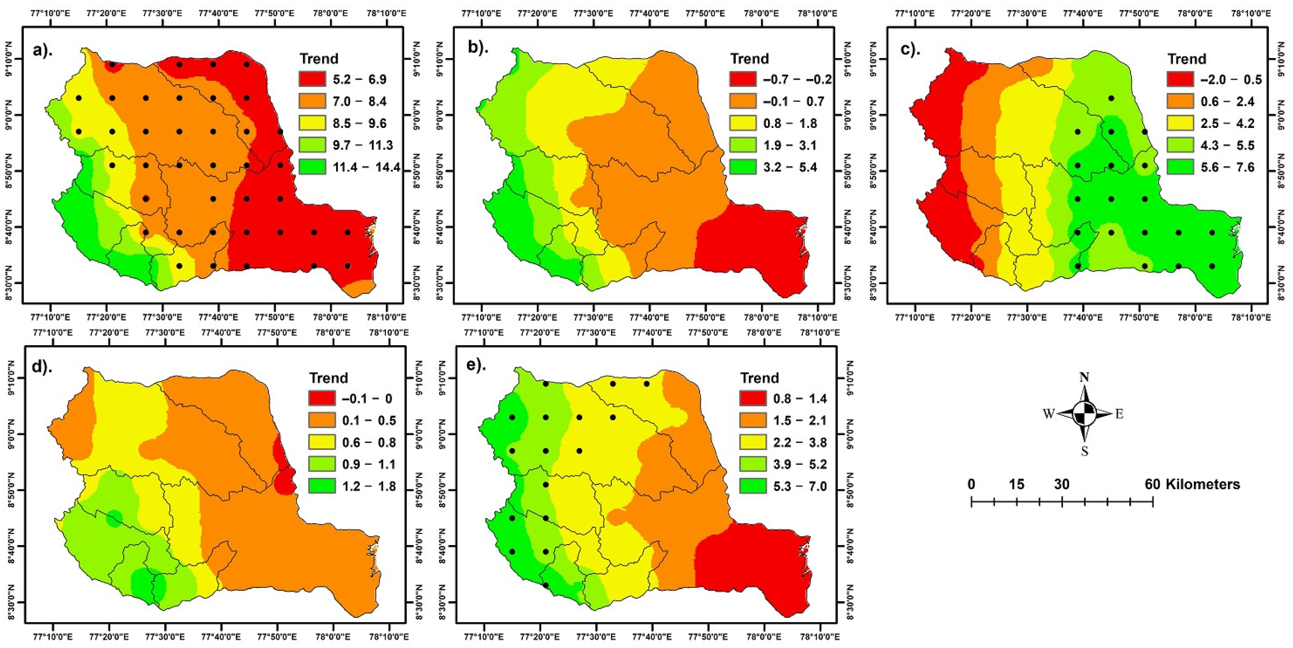
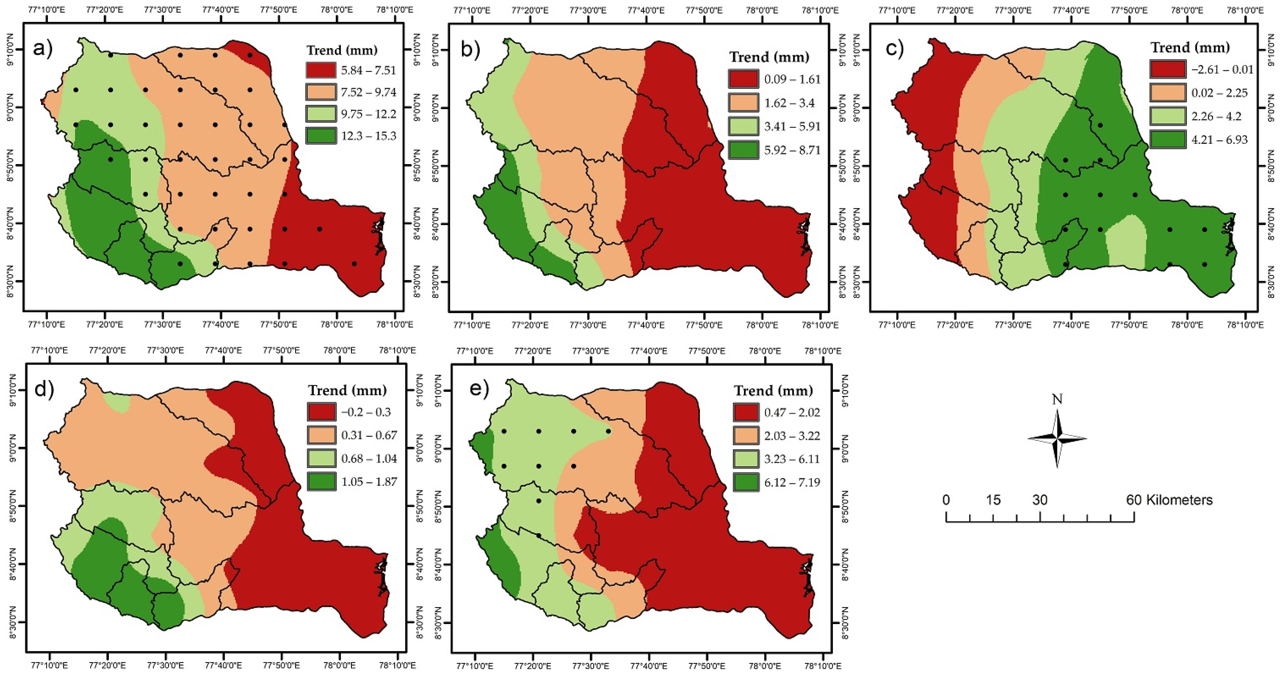
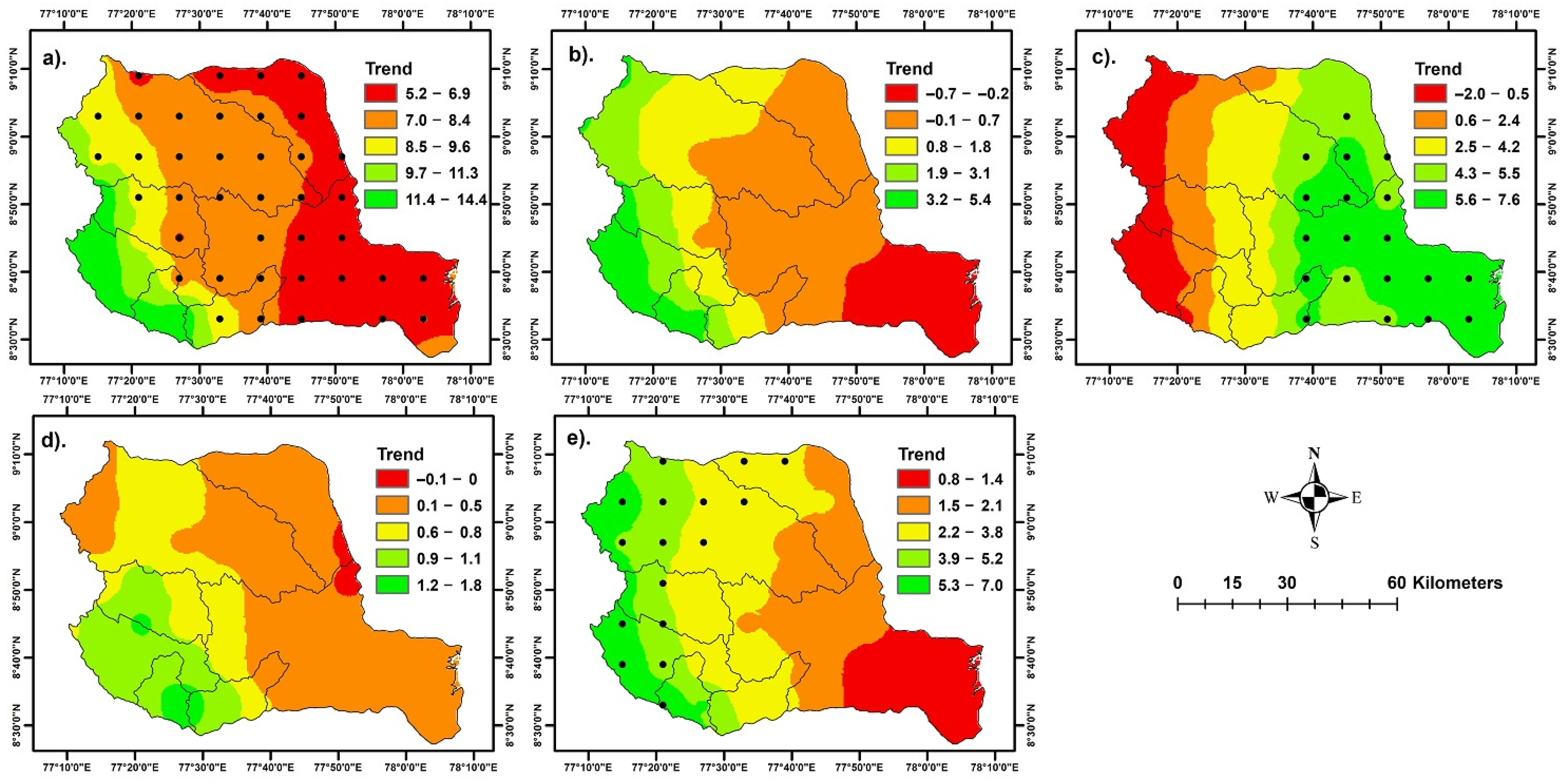
Rainfall trend analysis by MK, TFPW-MK, and ITA methods revealed heterogeneous results. Except for a few stations in the summer, the MK and TPFPW-MK trend analysis in gauge stations found no significant trend; however, in the ITA method, more than 60% of stations showed a significantly positive increase in rainfall (Table A2 and Table A3). The spatial pattern of the rainfall trend is given in Figure 9, Figure 10 and Figure 11. The comparison of spatial annual and seasonal rainfall trends revealed that the rainfall trends for the SWM, winter and summer rainfall are similar to the annual trend, with the trend being higher in the western regions than in the low plains, particularly the Lower Thamirabharani sub-basin in the basin’s east. The low plain zones only show a statistically significant rising tendency. Meanwhile, the rising trend in summer rainfall does not affect annual rainfall because the western half of the basin experiences a statistically significant increase in summer rainfall, but the same region does not see significant increases in yearly precipitation. This overall observed trend is similar to research conducted over major rivers in India [32]. The SWM does not show any significant rising tendency across the entire basin. During the NEM season, the low plains in the eastern part of the basin receive more rainfall and a significantly increased trend in the rainfall. Though the NEM is a major contributor of rainfall in the basin, especially the low plains areas might have intensive agriculture. It was also reported that the increase in rainfall during the NEM also increases the electrical conductivity and turbidity of water in the basin [94]. 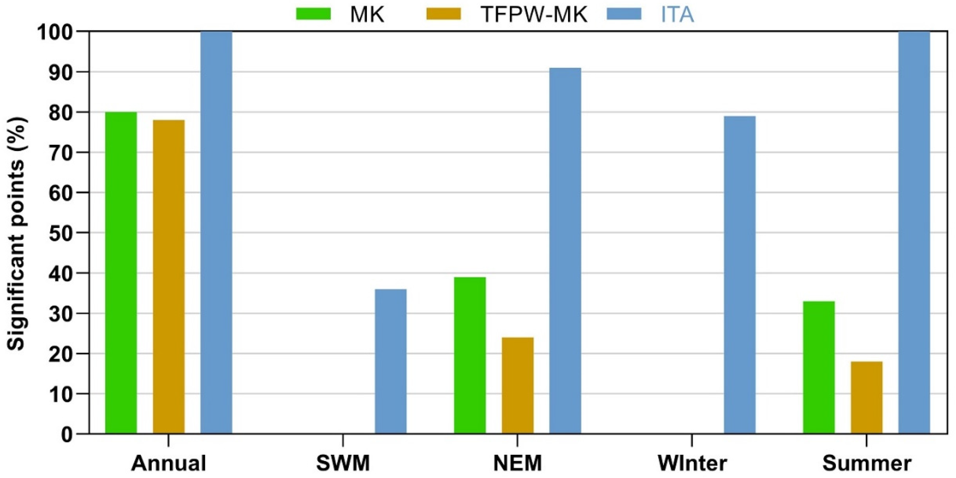The topography and monsoon activity both impact the rainfall pattern and trends in the Thamirabharani river basin [82]. The percentage of significant points was higher in the ITA approach than with the other methods (Figure 12). This confirms the research results that the ITA method has a greater advantage in detecting trends that the MK trend analysis did not detect [29,45]. However, the percentage of significant points was lesser in the trend-free prewhitening test, which might be due to the removal of serial correlation in the data.

Generally, spatiotemporal investigation of the seasonal contribution of rainfall in annual rainfall indicated that small regions in the basin’s western part have a significant rising trend in the summer. A significant upward trend was observed during the NEM over the central and southeast part of the basin, including the Lower Thamirabharani sub-basin. However, except during the NEM, the contribution of other seasonal trends to annual precipitation does not show a significant trend. Moreover, the results show that the contribution of each season to total annual rainfall varies between seasons in some parts of the basin. The results indicate that rainfall that occurs over the central, eastern, and southeast regions of the Thamirabharani basin during the NEM season, especially in the months of October, November, and December, could decrease in catchment areas and increase in the low plains of the basin.

5. Conclusions

Satellite-gridded data offered considerable potential for improving spatial aspects. Due to the significant variations of rainfall in monsoon-dependent areas, analyzing precipitation patterns in these locations is essential for effective water management planning. The current study used gridded satellite data as well as station data to analyze rainfall patterns and variability in the Thamirabharani river basin. The results indicated a good agreement between ground station data and satellite-gridded data. Spatiotemporal representation had greater variance and improved the identification of regional heterogeneity of trend and variability compared with gauge station data.

• The amount of annual rainfall received is higher in the western part of the basin than in the central and southeastern parts of the basin. The coastal, low-lying southeastern part of the basin gets more rainfall during the retreating monsoon.
• Variability in the annual rainfall across the basin is moderate and varies greatly from high to extremely high during the winter and summer, respectively.
• The monthly distribution of rainfall shows a moderate distribution in the western and central parts of the basin, where there was an anomalous distribution in the coastal regions.
• Trend analysis using the MK, TFPW-MK, and ITA methods revealed rising yearly rainfall in the basin’s low plains and coastal zones, with larger seasonal changes noted in the Lower Thamirabharani sub-basin. The annual rainfall pattern is influenced by the rainfall increasing tendency of the NEM and the summer season. Rainfall trends in SWM and winter were not statistically significant.
• Comparatively, on the annual and seasonal scale, the ITA method found trends that the MK and TFPW-MK tests did not. The Lower Thamirabharani sub-basin in the eastern half of the basin receives more rain throughout the NEM season than in other locations.
• To summarize, the low plains in the central part and coastal regions in the southeast experience increased rainfall with erratic monthly rainfall distribution; agricultural crop planning and water management planning should be undertaken properly in accordance with cyclonic activity.

References

1. Tripathi, A.K.; Pandey, P.C.; Sharma, J.K.; Triantakonstantis, D.; Srivastava, P.K. Climate Change and Its Impact on Forest of Indian Himalayan Region: A Review. Clim. Chang. 2022, 207–222. [Google Scholar] [CrossRef]
2. Milly, P.C.; Dunne, K.A. Potential evapotranspiration and continental drying. Nat. Clim. Change 2016, 6, 946–949. [Google Scholar] [CrossRef]
3. Kumar, N.; Khamzina, A.; Knöfel, P.; Lamers, J.P.A.; Tischbein, B. Afforestation of Degraded Croplands as a Water-Saving Option in Irrigated Region of the Aral Sea Basin. Water 2021, 13, 1433. [Google Scholar] [CrossRef]
4. Kim, J.; Kang, J. Analysis of flood damage in the Seoul Metropolitan government using climate change scenarios and mitigation technologies. Sustainability 2020, 13, 105. [Google Scholar] [CrossRef]
5. Alifujiang, Y.; Abuduwaili, J.; Maihemuti, B.; Emin, B.; Groll, M. Innovative trend analysis of precipitation in the Lake Issyk-Kul Basin, Kyrgyzstan. Atmosphere 2020, 11, 332. [Google Scholar] [CrossRef] [Green Version]
6. Toure, A.; Diekkrüger, B.; Mariko, A. Impact of climate change on groundwater resources in the Klela basin, southern Mali. Hydrology 2016, 3, 17. [Google Scholar] [CrossRef] [Green Version]
7. Wasko, C.; Nathan, R. Influence of changes in rainfall and soil moisture on trends in flooding. J. Hydrol. 2019, 575, 432–441. [Google Scholar] [CrossRef]
8. Abbot, J.; Marohasy, J. Skilful rainfall forecasts from artificial neural networks with long duration series and single-month optimization. Atmos. Res. 2017, 197, 289–299. [Google Scholar] [CrossRef]
9. Muthoni, F.K.; Baijukya, F.; Bekunda, M.; Sseguya, H.; Kimaro, A.; Alabi, T.; Mruma, S.; Hoeschle-Zeledon, I. Accounting for correlation among environmental covariates improves delineation of extrapolation suitability index for agronomic technological packages. Geocarto Int. 2019, 34, 368–390. [Google Scholar] [CrossRef] [Green Version]
10. Liu, Y.; Yuan, X.; Guo, L.; Huang, Y.; Zhang, X. Driving force analysis of the temporal and spatial distribution of flash floods in Sichuan Province. Sustainability 2017, 9, 1527. [Google Scholar] [CrossRef]
11. Zampieri, M.; Ceglar, A.; Dentener, F.; Toreti, A. Wheat yield loss attributable to heat waves, drought and water excess at the global, national and subnational scales. Environ. Res. Lett. 2017, 12, 64008. [Google Scholar] [CrossRef]
12. Skendžić, S.; Zovko, M.; Živković, I.P.; Lešić, V.; Lemić, D. The impact of climate change on agricultural insect pests. Insects 2021, 12, 440. [Google Scholar] [CrossRef] [PubMed]
13. Shahzad, A.; Ullah, S.; Dar, A.A.; Sardar, M.F.; Mehmood, T.; Tufail, M.A.; Shakoor, A.; Haris, M. Nexus on climate change: Agriculture and possible solution to cope future climate change stresses. Environ. Sci. Pollut. Res. 2021, 28, 14211–14232. [Google Scholar] [CrossRef]
14. Hu, W.; Wang, Y.; Li, H.; Huang, M.; Hou, M.; Li, Z.; She, D.; Si, B.J. Dominant role of climate in determining spatio-temporal distribution of potential groundwater recharge at a regional scale. J. Hydrol. 2019, 578, 124042. [Google Scholar] [CrossRef]
15. Tabari, H. Climate change impact on flood and extreme precipitation increases with water availability. Sci. Rep. 2020, 10, 13768. [Google Scholar] [CrossRef] [PubMed]
16. Bernstein, L.; Bosch, P.; Canziani, O.; Chen, Z.; Christ, R.; Riahi, K. IPCC, 2007: Climate Change 2007: Synthesis Report; IPCC: Geneva, Switzerland, 2008. [Google Scholar]
17. Gulizia, C.; Camilloni, I. A spatio-temporal comparative study of the representation of precipitation over South America derived by three gridded data sets. Int. J. Clim. 2016, 36, 1549–1559. [Google Scholar] [CrossRef]
18. Sidău, M.R.; Croitoru, A.-E.; Alexandru, D.-E. Comparative Analysis between Daily Extreme Temperature and Precipitation Values Derived from Observations and Gridded Datasets in North-Western Romania. Atmosphere 2021, 12, 361. [Google Scholar] [CrossRef]
19. Wong, C.L.; Liew, J.; Yusop, Z.; Ismail, T.; Venneker, R.; Uhlenbrook, S. Rainfall characteristics and regionalization in Peninsular Malaysia based on a high resolution gridded data set. Water 2016, 8, 500. [Google Scholar] [CrossRef] [Green Version]
20. Wang, F.; Yang, H.; Wang, Z.; Zhang, Z.; Li, Z. Drought evaluation with CMORPH satellite precipitation data in the Yellow River Basin by using gridded standardized precipitation evapotranspiration index. Remote Sens. 2019, 11, 485. [Google Scholar] [CrossRef] [Green Version]
21. Mondal, A.; Lakshmi, V.; Hashemi, H. Intercomparison of trend analysis of multisatellite monthly precipitation products and gauge measurements for river basins of India. J. Hydrol. 2018, 565, 779–790. [Google Scholar] [CrossRef]
22. Irannezhad, M.; Liu, J. Evaluation of six gauge-based gridded climate products for analyzing long-term historical precipitation patterns across the Lancang-Mekong River Basin. Geogr. Sustain. 2022, 3, 85–103. [Google Scholar] [CrossRef]
23. Kumar, M.; Hodnebrog, Ø.; Daloz, A.S.; Sen, S.; Badiger, S.; Krishnaswamy, J. Measuring precipitation in Eastern Himalaya: Ground validation of eleven satellite, model and gauge interpolated gridded products. J. Hydrol. 2021, 599, 126252. [Google Scholar] [CrossRef]
24. Baudouin, J.-P.; Herzog, M.; Petrie, C.A. Cross-validating precipitation datasets in the Indus River basin. Hydrol. Earth Syst. Sci. 2020, 24, 427–450. [Google Scholar] [CrossRef] [Green Version]
25. Gedefaw, M.; Yan, D.; Wang, H.; Qin, T.; Girma, A.; Abiyu, A.; Batsuren, D. Innovative trend analysis of annual and seasonal rainfall variability in Amhara regional state, Ethiopia. Atmosphere 2018, 9, 326. [Google Scholar] [CrossRef] [Green Version]
26. Mosaffa, H.; Sadeghi, M.; Hayatbini, N.; Afzali Gorooh, V.; Akbari Asanjan, A.; Nguyen, P.; Sorooshian, S. Spatiotemporal variations of precipitation over Iran using the high-resolution and nearly four decades satellite-based PERSIANN-CDR dataset. Remote Sens. 2020, 12, 1584. [Google Scholar] [CrossRef]
27. Bhattacharyya, S.; Sreekesh, S.; King, A. Characteristics of extreme rainfall in different gridded datasets over India during 1983–2015. Atmos. Res. 2022, 267, 105930. [Google Scholar] [CrossRef]
28. Sharma, S.; Chen, Y.; Zhou, X.; Yang, K.; Li, X.; Niu, X.; Hu, X.; Khadka, N. Evaluation of GPM-Era satellite precipitation products on the southern slopes of the Central Himalayas against rain gauge data. Remote Sens. 2020, 12, 1836. [Google Scholar] [CrossRef]
29. Malik, A.; Kumar, A. Spatio-temporal trend analysis of rainfall using parametric and non-parametric tests: Case study in Uttarakhand, India. Theor. Appl. Climatol. 2020, 140, 183–207. [Google Scholar] [CrossRef]
30. Zakwan, M.; Ara, Z. Statistical analysis of rainfall in Bihar. Sustain. Water Resour. Manag. 2019, 5, 1781–1789. [Google Scholar] [CrossRef]
31. Velasco-Forero, C.A.; Sempere-Torres, D.; Cassiraga, E.F.; Gómez-Hernández, J.J. A non-parametric automatic blending methodology to estimate rainfall fields from rain gauge and radar data. Adv. Water Resour. 2009, 32, 986–1002. [Google Scholar] [CrossRef]
32. Mondal, A.; Khare, D.; Kundu, S. Spatial and temporal analysis of rainfall and temperature trend of India. Theor. Appl. Climatol. 2015, 122, 143–158. [Google Scholar] [CrossRef]
33. Şen, Z. Innovative trend analysis methodology. J. Hydrol. Eng. 2012, 17, 1042–1046. [Google Scholar] [CrossRef]
34. Chen, Y.; Guan, Y.; Shao, G.; Zhang, D. Investigating trends in streamflow and precipitation in Huangfuchuan Basin with wavelet analysis and the Mann-Kendall test. Water 2016, 8, 77. [Google Scholar] [CrossRef] [Green Version]
35. Ali, R.; Kuriqi, A.; Abubaker, S.; Kisi, O. Long-term trends and seasonality detection of the observed flow in Yangtze River using Mann-Kendall and Sen’s innovative trend method. Water 2019, 11, 1855. [Google Scholar] [CrossRef] [Green Version]
36. Tan, M.L.; Samat, N.; Chan, N.W.; Lee, A.J.; Li, C. Analysis of precipitation and temperature extremes over the Muda River Basin, Malaysia. Water 2019, 11, 283. [Google Scholar] [CrossRef] [Green Version]
37. Patakamuri, S.K.; Muthiah, K.; Sridhar, V. Long-term homogeneity, trend, and change-point analysis of rainfall in the arid district of Ananthapuramu, Andhra Pradesh State, India. Water 2020, 12, 211. [Google Scholar] [CrossRef] [Green Version]
38. Sediqi, M.N.; Shiru, M.S.; Nashwan, M.S.; Ali, R.; Abubaker, S.; Wang, X.; Ahmed, K.; Shahid, S.; Asaduzzaman, M.; Manawi, S.M.A. Spatio-temporal pattern in the changes in availability and sustainability of water resources in Afghanistan. Sustainability 2019, 11, 5836. [Google Scholar] [CrossRef] [Green Version]
39. Shiru, M.S.; Shahid, S.; Alias, N.; Chung, E.-S. Trend analysis of droughts during crop growing seasons of Nigeria. Sustainability 2018, 10, 871. [Google Scholar] [CrossRef] [Green Version]
40. Fan, J.; Sun, W.; Zhao, Y.; Xue, B.; Zuo, D.; Xu, Z. Trend analyses of extreme precipitation events in the Yarlung zangbo river basin, China using a high-resolution precipitation product. Sustainability 2018, 10, 1396. [Google Scholar] [CrossRef] [Green Version]
41. Şen, Z. Trend identification simulation and application. J. Hydrol. Eng. 2014, 19, 635–642. [Google Scholar] [CrossRef]
42. Öztopal, A.; Şen, Z. Innovative trend methodology applications to precipitation records in Turkey. Water Resour. Manag. 2017, 31, 727–737. [Google Scholar] [CrossRef]
43. Almazroui, M.; Şen, Z. Trend analyses methodologies in hydro-meteorological records. Earth Syst. Environ. 2020, 4, 713–738. [Google Scholar] [CrossRef]
44. Tian, Y.; Yan, Z.; Li, Z. Spatial and Temporal Variations of Extreme Precipitation in Central Asia during 1982–2020. Atmosphere 2021, 13, 60. [Google Scholar] [CrossRef]
45. Malik, A.; Kumar, A.; Guhathakurta, P.; Kisi, O. Spatial-temporal trend analysis of seasonal and annual rainfall (1966–2015) using innovative trend analysis method with significance test. Arab. J. Geosci. 2019, 12, 328. [Google Scholar] [CrossRef]
46. Harka, A.E.; Jilo, N.B.; Behulu, F. Spatial-temporal rainfall trend and variability assessment in the Upper Wabe Shebelle River Basin, Ethiopia: Application of innovative trend analysis method. J. Hydrol. Reg. Stud. 2021, 37, 100915. [Google Scholar] [CrossRef]
47. Krakauer, N.Y.; Lakhankar, T.; Dars, G.H. Precipitation trends over the Indus basin. Climate 2019, 7, 116. [Google Scholar] [CrossRef] [Green Version]
48. Larbi, I.; Hountondji, F.C.; Annor, T.; Agyare, W.A.; Mwangi Gathenya, J.; Amuzu, J. Spatio-temporal trend analysis of rainfall and temperature extremes in the Vea Catchment, Ghana. Climate 2018, 6, 87. [Google Scholar] [CrossRef] [Green Version]
49. Mulugeta, S.; Fedler, C.; Ayana, M. Analysis of long-term trends of annual and seasonal rainfall in the Awash river basin, Ethiopia. Water 2019, 11, 1498. [Google Scholar] [CrossRef] [Green Version]
50. Srivastava, P.K.; Pradhan, R.K.; Petropoulos, G.P.; Pandey, V.; Gupta, M.; Yaduvanshi, A.; Wan Jaafar, W.Z.; Mall, R.K.; Sahai, A.K. Long-term trend analysis of precipitation and extreme events over Kosi river basin in India. Water 2021, 13, 1695. [Google Scholar] [CrossRef]
51. Raju, B.C.K.; Nandagiri, L. Analysis of historical trends in hydrometeorological variables in the upper Cauvery Basin, Karnataka, India. Curr. Sci. 2017, 112, 577–587. [Google Scholar] [CrossRef]
52. Sreelash, K.; Mathew, M.M.; Nisha, N.; Arulbalaji, P.; Bindu, A.G.; Sharma, R.K. Changes in the Hydrological Characteristics of Cauvery River draining the eastern side of southern Western Ghats, India. Int. J. River Basin Manag. 2020, 18, 153–166. [Google Scholar] [CrossRef]
53. Gowri, R.; Dey, P.; Mujumdar, P.P. A hydro-climatological outlook on the long-term availability of water resources in Cauvery river basin. Water Secur. 2021, 14, 100102. [Google Scholar] [CrossRef]
54. Kalyan, A.V.S.; Ghose, D.K.; Thalagapu, R.; Guntu, R.K.; Agarwal, A.; Kurths, J.; Rathinasamy, M. Multiscale spatiotemporal analysis of extreme events in the Gomati River Basin, India. Atmosphere 2021, 12, 480. [Google Scholar] [CrossRef]
55. NWC. Action Plan on Rejuvenation of River Thamirabarani Pappankulam to Arumuganeri Stretch; Tamil Nadu Pollution Control Board: Chennai, India, 2017.
56. Geethalakshmi, V.; McBride, J.; Huda, S. Impact of ENSO on Tamil Nadu rainfall. J. Meteorol. 2005, 29, 9–16. [Google Scholar]
57. Malarvizhi, R.; Ravikumar, G. Statistical research on rainfall and river discharge patterns over time from a hydrological perspective. Appl. Ecol. Environ. Res. 2021, 19, 2091–2110. [Google Scholar] [CrossRef]
58. Isabella, M.M.; Ambujam, N.K.; Krishnan, S. Trend analysis of streamflow and its relation to rainfall in the lower tamiraparani sub-basin of Tamilnadu, India. Appl. Ecol. Environ. Res. 2020, 18, 863–878. [Google Scholar] [CrossRef]
59. WRD. Tamil Nadu—Irrigated Agriculture Modernization and Water-Bodies Restoration and Management Project; Water Resource Organiztion: Chennai, India, 2008.
60. CPG. Crop Production Guide; Directorate of Agriculture, Government of Tamil Nadu and Tamil Nadu Agricultural University: Coimbatore, India, 2020. [Google Scholar]
61. Yadav, B.P.; Saxena, R.; Das, A.K.; Bharwani, H.M. Standard Operation Procedures (SOP) for Hydromet Services; India Meteorological Department: New Delhi, India, 2021.
62. Attri, S.D.; Tyagi, A. Climate Profile of India; Environment Monitoring and Research Center, India Meteorology Department: New Delhi, India, 2010.
63. Beck, H.E.; Wood, E.F.; Pan, M.; Fisher, C.K.; Miralles, D.G.; Van Dijk, A.I.; McVicar, T.R.; Adler, R.F. MSWEP V2 global 3-hourly 0.1 precipitation: Methodology and quantitative assessment. Bull. Am. Meteorol. Soc. 2019, 100, 473–500. [Google Scholar] [CrossRef] [Green Version]
64. Beck, H.E.; Pan, M.; Roy, T.; Weedon, G.P.; Pappenberger, F.; van Dijk, A.I.J.M.; Huffman, G.J.; Adler, R.F.; Wood, E.F. Daily evaluation of 26 precipitation datasets using Stage-IV gauge-radar data for the CONUS. Hydrol. Earth Syst. Sci. 2019, 23, 207–224. [Google Scholar] [CrossRef] [Green Version]
65. Prakash, S. Performance assessment of CHIRPS, MSWEP, SM2RAIN-CCI, and TMPA precipitation products across India. J. Hydrol. 2019, 571, 50–59. [Google Scholar] [CrossRef]
66. Nair, A.S.; Indu, J. Performance assessment of multi-source weighted-ensemble precipitation (MSWEP) product over India. Climate 2017, 5, 2. [Google Scholar] [CrossRef]
67. Childs, C. Interpolating surfaces in ArcGIS spatial analyst. ArcUser July Sept. 2004, 3235, 32–35. [Google Scholar]
68. Asfaw, A.; Simane, B.; Hassen, A.; Bantider, A. Variability and time series trend analysis of rainfall and temperature in northcentral Ethiopia: A case study in Woleka sub-basin. Weather Clim. Extrem. 2018, 19, 29–41. [Google Scholar] [CrossRef]
69. Pandey, V.; Srivastava, P.K.; Singh, S.K.; Petropoulos, G.P.; Mall, R.K. Drought identification and trend analysis using long-term CHIRPS satellite precipitation product in Bundelkhand, India. Sustainability 2021, 13, 1042. [Google Scholar] [CrossRef]
70. Oliver, J.E. Monthly precipitation distribution: A comparative index. Prof. Geogr. 1980, 32, 300–309. [Google Scholar] [CrossRef]
71. Mann, H.B. Nonparametric tests against trend. Econom. J. Econom. Soc. 1945, 13, 245–259. [Google Scholar] [CrossRef]
72. Kendall, M.G. Rank Correlation Methods; American Psychological Association: Washington, DC, USA, 1948. [Google Scholar]
73. Sen, P.K. Estimates of the regression coefficient based on Kendall’s tau. J. Am. Stat. Assoc. 1968, 63, 1379–1389. [Google Scholar] [CrossRef]
74. Alahacoon, N.; Edirisinghe, M. Spatial variability of rainfall trends in Sri Lanka from 1989 to 2019 as an indication of climate change. ISPRS Int. J. Geo Inf. 2021, 10, 84. [Google Scholar] [CrossRef]
75. Koudahe, K.; Kayode, A.J.; Samson, A.O.; Adebola, A.A.; Djaman, K. Trend analysis in standardized precipitation index and standardized anomaly index in the context of climate change in Southern Togo. Atmos. Clim. Sci. 2017, 7, 401. [Google Scholar] [CrossRef] [Green Version]
76. von Storch, H. Misuses of Statistical Analysis in Climate Research. In Analysis of Climate Variability: Applications of Statistical Techniques; von Storch, H., Navarra, A., Eds.; Springer: Berlin/Heidelberg, Germany, 1995; pp. 11–26. [Google Scholar]
77. Kulkarni, A.; von Storch, H. Monte Carlo experiments on the effect of serial correlation on the Mann-Kendall test of trend. Meteorol. Z. 1995, 4, 82–85. [Google Scholar] [CrossRef]
78. Yue, S.; Pilon, P.; Phinney, B.; Cavadias, G. The influence of autocorrelation on the ability to detect trend in hydrological series. Hydrol. Process. 2002, 16, 1807–1829. [Google Scholar] [CrossRef]
79. Şen, Z. Innovative trend significance test and applications. Theor. Appl. Climatol. 2017, 127, 939–947. [Google Scholar] [CrossRef]
80. Misra, V.; Bhardwaj, A. Defining the Northeast Monsoon of India. Mon. Weather Rev. 2019, 147, 791–807. [Google Scholar] [CrossRef]
81. Veeraputhiran, R.; Karthikeyan, R.; Geethalakshmi, V.; Selvaraju, R.; Sundarsingh, S.D.; Balasubramaniyan, T.N. Crop Planning–Climate Atlas, Manual. A. E. Publications: Coimbatore, India, 2003; pp. 45–49. [Google Scholar]
82. Rajalakshmi, D.; Jagannathan, R.; Geethalakshmi, V. Future Climate Uncertainty And Spatial Variability Over Tamilnadu State, India. Glob. Nest J. 2015, 17, 175–185. [Google Scholar]
83. Sivapragasam, C.; Balamurli, S.; Deepak, M.; Prakhar, A.; Muttil, N. Trends in rainfall patterns over the Tamarabarani basin in Tamil Nadu, India. In Proceedings of the 20th International Congress on Modelling and Simulation, Adelaide, Australia, 1–6 December 2013; pp. 2583–2589. [Google Scholar]
84. Palaniswami, S.; Muthiah, K. Change Point Detection and Trend Analysis of Rainfall and Temperature Series over the Vellar River Basin. Polish J. Environ. Stud. 2018, 27, 1673–1681. [Google Scholar] [CrossRef]
85. Anand, B.; Karunanidhi, D. Long term spatial and temporal rainfall trend analysis using GIS and statistical methods in Lower Bhavani basin, Tamil Nadu, India. Indian J. Geo-Mar. Sci. 2020, 49, 419–427. [Google Scholar]
86. Vengateswari, M.; Geethalakshmi, V.; Bhuvaneswari, K.; Panneerselvam, S. Influence of ENSO on wet and dry spell frequency for rainfed cropping period over Tamil Nadu. Int. Arch. Photogramm. Remote Sens. Spat. Inf. Sci. 2019, 42, 63–65. [Google Scholar] [CrossRef] [Green Version]
87. Geethalakshmi, V.; Lakshmanan, A.; Rajalakshmi, D.; Jaganathan, R.; Sridhar, G.; Ramaraj, A.P. Climate change impacts assessment and adaption strategies to sustain rice production in Cauvery basin of Tamil Nadu. Curr. Sci. 2011, 101, 342–347. [Google Scholar]
88. Hrudya, P.H.; Varikoden, H.; Vishnu, R. A review on the Indian summer monsoon rainfall, variability and its association with ENSO and IOD. Meteorol. Atmos. Phys. 2021, 133, 1–14. [Google Scholar] [CrossRef]
89. Rajendran, K.; Kitoh, A.; Srinivasan, J.; Mizuta, R.; Krishnan, R. Monsoon circulation interaction with Western Ghats orography under changing climate. Theor. Appl. Climatol. 2012, 110, 555–571. [Google Scholar] [CrossRef]
90. Bayable, G.; Amare, G.; Alemu, G.; Gashaw, T. Spatiotemporal variability and trends of rainfall and its association with Pacific Ocean Sea surface temperature in West Harerge Zone, Eastern Ethiopia. Environ. Syst. Res. 2021, 10, 7. [Google Scholar] [CrossRef]
91. Guna, M.; Ramanathan, S.P.; Geethalakshmi, V.; Chandrakumar, K.; Kokilavani, S.; Djanaguiraman, M. Effect of high night temperature and CO2 on yield and seed quality of summer green gram (Vigna radiata) under soil plant atmospheric research (SPAR). J. Agrometeorol. 2022, 24, 229–234. [Google Scholar] [CrossRef]
92. Ramasamy, G.; Geethalakshmi, V.; Kumar, N.; Lakshmanan, A.; Bhuvaneswari, K.; Dheebakaran, G.A.; Senthilraja, K. Drought analysis and management for Tamil Nadu: Science-stakeholder-policy linkage. J. Agrometeorol. 2020, 22, 429–438. [Google Scholar]
93. Zhang, K.; Yao, Y.; Qian, X.; Wang, J. Various characteristics of precipitation concentration index and its cause analysis in China between 1960 and 2016. Int. J. Climatol. 2019, 39, 4648–4658. [Google Scholar] [CrossRef]
94. Ravichandran, S. Hydrological influences on the water quality trends in Tamiraparani Basin, South India. Environ. Monit. Assess. 2003, 87, 293–309. [Google Scholar] [CrossRef]
Figure 1. Flowchart of the overall methodology used for studying rainfall variability and trends in the Thamirabharani river basin.
Sustainability 14 14948 g001
Figure 2. Location of the study area. (a) Location of the Thamirabharani river basin in southern part of Tamil Nadu. (b) Land-use and land cover map of the Thamirabharani river basin. (c) Map showing the location of rain gauge station, MSWEP data points, and sub-basins. (d). Topographic map showing elevation (m) from mean sea level.
Sustainability 14 14948 g002
Figure 3. MSWEP mean annual rainfall (mm) of the Thamirabharani basin from 1991 to 2020.
Sustainability 14 14948 g003
Figure 4. MSWEP mean seasonal rainfall (mm) of the Thamirabharani basin from 1991 to 2020. (a) SWM season, (b) NEM season, (c) winter season, and (d) summer season.
Sustainability 14 14948 g004
Figure 5. Spatial variation of coefficient of variation (CV) in rainfall over Thamirabharani basin. (a) Annual, (b) SWM, (c) NEM, (d) winter, and (e) summer season.
Sustainability 14 14948 g005
Figure 6. A heat map shows the yearly PCI values at each station. CPD—consistent precipitation distribution (White), MPD—moderate precipitation distribution (Green), APD—anomalous precipitation distribution (Blue), and IPD—irregular precipitation distribution (Red) of rainfall.
Sustainability 14 14948 g006
Figure 7. The graph shows the number of years with MPD, APD, and IPD of rainfall events observed in the Thamirabharani river basin from 1991 to 2020.
Sustainability 14 14948 g007
Figure 8. Distribution of annual mean PCI values (1991–2020) across the Thamirabharani river basin.
Sustainability 14 14948 g008
Figure 9. Slope of trend (mm/year) by Mann-Kendall test in annual and seasonal rainfall over the Thamirabharani river basin. (a)Annual, (b) SWM, (c) NEM, and (d) winter (e) summer season. Black dot points on map represent the significance (Zmk > 1.96) at p = 0.05.
Sustainability 14 14948 g009
Figure 10. Slope of trend (mm/year) by trend-free prewhitening Mann-Kendall test in annual and seasonal rainfall over the Thamirabharani river basin. (a) Annual, (b) SWM, (c) NEM, (d) winter, and (e) summer season. Black dot points on map represent the significance (Z > 1.96) at p = 0.05.
Sustainability 14 14948 g010
Figure 11. Trend slope (TS) (mm/year) over the Thamirabharani river basin. (a) Annual, (b) SWM, (c) NEM, (d) winter, and (e) summer season. Black dot points on map represent the significance at p = 0.05.
Sustainability 14 14948 g011
Figure 12. Comparison of the percentage of significant points by trend analysis methods.
Sustainability 14 14948 g012