Article

Performance Assessment of Global Horizontal Irradiance Models in All-Sky Conditions

Department of Mechanical Engineering, Kookmin University, 77 Jeongneung-ro, Seongbuk-gu, Seoul 02727, Korea
*
Author to whom correspondence should be addressed.
Energies 2021, 14(23), 7939; https://doi.org/10.3390/en14237939
Submission received: 27 September 2021 / Revised: 2 November 2021 / Accepted: 22 November 2021 / Published: 26 November 2021
(This article belongs to the Special Issue Simulation Modelling and Analysis of a Renewable Energy System)

Abstract

:
Solar irradiance models contribute to mitigating the lack of measurement data at a ground station. Conventionally, the models relied on physical calculations or empirical correlations. Recently, machine learning as a sophisticated statistical method has gained popularity due to its accuracy and potential. While some studies compared machine learning models with other models, a study has not yet been performed that compares them side-by-side to assess their performance using the same datasets in different locations. Therefore, this study aims to evaluate the accuracy of three representative models for estimating solar irradiance using atmospheric variables measurement and cloud amount derived from satellite images as the input parameters. Based on its applicability and performance, this study selected the fast all-sky radiation model for solar applications (FARMS) derived from the radiative transfer approach, the Hammer model that simplified atmospheric correlation, and the long short-term memory (LSTM) model specialized in sequential datasets. Global horizontal irradiance (GHI) data were modeled for five distinct locations in South Korea and compared with hourly measurement data of two years to yield the error metrics. When identical input parameters were used, LSTM outperformed the FARMS and the Hammer model in terms of relative root mean square difference (rRMSD) and relative mean bias difference (rMBD). Training an LSTM model using the input parameters of FARMS, such as ozone, nitrogen, and precipitable water, yielded more accurate results than using the Hammer model. The result shows unbiased and accurate estimation with an rRMSD and rMBD of 23.72% and 0.14%, respectively. Conversely, the FARMS has a faster processing speed and does not require significant data to make a fair estimation.

Graphical Abstract

1. Introduction

With photovoltaic technology leading the escalating integration of renewable sources into domestic and industrial clusters, accurate estimation of global horizontal irradiance (GHI) becomes an important challenge since it can easily correlate to solar generation performance [1]. However, due to constant fluctuations in the weather and the earth’s atmospheric conditions, estimating solar power generation is frequently unpredictable [2].
Solar radiation reaching the ground is scattered, absorbed, or transmitted by intervening atmospheric variables such as ozone, ambient pressure, and precipitable water [3], but in particular, the most prominent effect is due to clouds [4]. A moving cloud with varying shading strength has been shown to change irradiance value by over 300 W/m2 in 0.1 s, implying that irradiance transitions produced by overpassing cloud shadows can be significant and severe [5]. Thus, reliable data that describe atmospheric conditions and cloudiness is essential to estimate GHI under certain times and locations.
Direct ground measurements with a pyranometer and pyrheliometer provide the most reliable solar irradiance data. Presently, solar irradiance measurement technology has progressed to real-time data that can be collected and monitored automatically. However, ground measurement systems are expensive and require careful maintenance. As a result, ground measurement has limited spatial coverage, and the measurement database remains inadequate to meet the needs of a solar power society. Despite some work attempting to use conventional methodologies, such as interpolation, to overcome the limited spatial coverage of direct measurement, the accuracy of the interpolated data is still inadequate [6,7]. Consequently, the data generally comes from an open-source database or an organization.
Although cloud cover is crucial observation data for global weather and climate, ground-based automatic recording has not been conducted in various countries, including Brazil, United States of America, and South Korea [8,9,10]. To put it another way, some cloud cover data (octa or tenth) has only been recorded through the eyes of a human observer and hence could be affected by the observer’s subjective judgment [11,12]. Observation data recorded by an unskilled observer, in particular, will contain multiple inaccuracies, lowering its quality [13,14].
Multiple studies have figured out a more reliable way to determine the cloud conditions based on easily accessible data (i.e., satellite images) [15,16,17]. Compared with human observation, the satellite-derived calculation is more precise when utilized for solar applications. A simple satellite model uses the visible channel of the satellite to calculate a cloud index ( CI ). The CI is then used to modulate a clear-sky global irradiance model. The satellite’s ability to reliably access information in any location around the globe is another notable feature of this method. Even though the absolute precision for any given location may not be perfect, satellites have proven to be a more reliable source of cloud detection than human observation.
The variability in cloud amount usually changes in each location, especially due to the fact that the level of humidity changes according to the climate [18]. As stated by Rubel et al. [19], the most widely used method of climate characterization is the work of Wladimir Köppen [20,21]. Based on seasonal precipitation and temperature trend, climates are classified into five main groups by the Köppen–Geiger climate classification. All climates were given a letter to symbolize each group, subgroup, and temperature conditions. Cwa, for example, denotes a temperate climate with dry winters and hot summers. Figure 1 shows the climate classification for South Korea.
Since each climate has its unique set of atmospheric conditions, the GHI model is divided based on three approaches: physical, semi-empirical, and statistical modelling; some results are summarized in Table 1. In order to avoid miscalculation due to less essential parameters, most physical models use physics-based calculations and regressive correlation. Once the coefficients of correlation equations have been determined, the model is easy to implement. Over time, the solar irradiance measurement models have been extensively revised. For example, Kasten et al. [22] proposed a model to connect cloud amounts to GHI. More GHI parameters, such as temperature, humidity, wind speed, and cloud level, were added by Zhang et al. [23]. Physical models that also simulate light scattering and absorption by air molecules and that are solved using a radiative transfer (RT) equation are called RT models (e.g., discrete ordinates RT [24], rapid RT model [25], and moderate resolution atmospheric transmission [26]). Although RT models have an adequate result in estimating solar irradiance, RT computations under certain cloudy skies are substantially more computationally expensive than standard physical models due to the complexity of solving the RT equation. As a result, a radiation model that inherits the computation ability of a physical model is needed. The fast all-sky radiation model for solar applications (FARMS) is one model that addresses these issues [27]. By precomputing cloud transmittance and reflectance into simulated lookup tables, this model improves on existing RT as it did not explicitly solve the RT equation for each cloud condition, which consumes considerable computational resources. As a consequence, the model’s computational time is greatly reduced.
Several computational methods for estimating GHI from satellite observations have been established in recent decades [6]. The Hammer model, developed after extensive field analysis and data collecting, has been used in several European studies to collect solar irradiance data for solar energy and daylight use [30]. In addition, recent developments in machine learning allow for sophisticated statistical approaches. Machine learning models are more accurate in complex physics because they estimate the mapping function from input to output variables. Several machine learning models, especially for GHI, have been successfully implemented [1]. Those methods that specialize in handling sequential or time-series data, such as text, voice, and image, have had a lot of success. Since solar forecasting is intrinsically based on sequential data, the most common models are the recurrent neural network (RNN), long short-term memory (LSTM), gated recurrent unit (GRU), and a convolutional neural network LSTM model. According to Ramadhan et al. [33], the LSTM model is the best sequential data set for solar applications.
GHI estimation is a challenging task, and many significant and crucial steps need consideration. Selecting the model for estimating GHI values is one of the essential steps in obtaining an accurate result. Hence, this work proposes a direct examination of the accuracy performance of the physical, semi-empirical, and machine learning models, using solar irradiance observation data, satellite images, and atmospheric conditions, for two years in Korea and at five different locations based on its Köppen–Geiger climate classifications. The models in this paper were chosen based on their performances and input variables, in which the FARMS, Hammer model, and LSTM model represent the physical, semi-empirical, and machine learning models, respectively. The machine learning model uses both the Hammer and the FARMS inputs.

2. Data Collection

The Korea Meteorological Administration (KMA) regularly measure solar irradiance over the northern hemisphere, including the Korean peninsula. The KMA uses a pyranometer to measure the amount of GHI at each station [9]. This study used in situ solar irradiance measurements from five KMA station locations, as shown in Table 2. These locations were chosen based on the Köppen–Geiger climate classification.
For model input, all KMA stations provided hourly cumulative GHI measurements (MJ/m2) that were divided by 3600 s to yield hourly GHI averages (W/m2). The measurement period for all KMA stations was from 1 January 2018 to 31 December 2019. Quality control was used in this analysis based on the technique established by Gueymard and Lave, to ensure accurate data from the ground measurements [35,36]. All accumulated data needed to follow the criteria outlined below, or the data were marked as invalid:
  • θ z   <   85 ° ;
  • GHI   >   0   W / m 2 ;
  • GHI   <   1 . 5 G ext cos 1 . 2 θ z + 100   W / m 2 .
The solar zenith angle and extraterrestrial irradiance on a normal surface, respectively, were denoted by θ z and G ext . Data that did not follow the criteria were discarded. Note that the GHI values at low sun elevation were removed using the θ z   <   85 ° criterion. As part of the KMA, the National Meteorological Satellite Center (NMSC) generates Communication, Ocean, and Meteorological Satellite (COMS) Level-1B data in five separate channels:
  • Visible (0.67 μm);
  • Shortwave infrared (3.7 μm);
  • Water vapor (6.7 μm);
  • Infrared (10.8 μm);
  • Infrared (12.0 μm).
The visible and infrared channels have horizontal resolutions of 1 and 4 km, respectively; the image radius covered all of the chosen sites on the Korean peninsula (32° N–40° N, 125° E–130° E) 291.92 km. The COMS images were collected hourly from 1 January 2018 to 31 December 2019.
The aerosol robotic network (AERONET) is a National Aeronautics and Space Administration (NASA) network of ground-based measurements that provides information on atmospheric conditions, such as ozone ( O 3 ), nitrogen concentration ( N 2 ), precipitable water ( W P ), optical thickness ( OT ), Angstrom coefficient ( α ), Angstrom turbidity ( β ), and pressure ( P ). The AERONET data have three levels of quality: level-1 data are raw measurement data that have not been filtered or normalized, level-1.5 data are filtered data, and level-2 data are filtered data that have been quality checked. Level-2 data were arranged hourly for a one-year period from 1 January 2018 to 31 December 2019. The AERONET measurement of O 3 was obtained according to a formula by Komhyr et al. [37], which uses ozone concentration ( C O 3 ) and the ozone optical air mass ( m O 3 ) from a total ozone mapping spectrometer (TOMS) [38]. Similarly, N 2 calculation uses the nitrogen concentration ( C N 2 ) and nitrogen coefficient ( α N 2 ) from an ozone monitoring instrument (OMI) [39]. A sun photometer (Cimel CE-318-4) was used to measure W P at different wavelengths using interference filters. Six filters were centered at 340, 380, 440, 670, 870, and 1020 nm. Since the majority of the variables in the proposed models come from a wavelength of 940 nm, data from the filters in the 870 to 1020 nm range were used. Further information and standardization of calibration regarding this instrument can be found in Holben et al. [40,41]. The Angstrom optical depth (AOD) at 935 nm was extrapolated using the angstrom coefficient and the turbidity was derived by a linear regression of the AOD and wavelengths within 870 nm, excluding the channels affected by water vapor [41]. To compute the local pressure, the National Center for Environmental Prediction (NCEP) analyzed mean sea level pressure at standard levels (1000, 925, 850, 700, and 600 hPa) and fitted to a quadratic function in logarithmic space [42]. Error in the local pressure is generally less than two hPa. Additionally, an aethalometer was used to determine the amount of optical thickness at seven different wavelengths [43].

3. Global Horizontal Irradiance Estimation

Based on their accuracy, versatility, and popularity, three models for estimating GHI was chosen in this study from three well-known methods: FARMS, the Hammer model, and LSTM [27,30,44]. The FARMS formula is constructed by combining two calculations, clear-sky and overcast, to estimate all-sky irradiance. The clear-sky computation is based on the reference evaluation of solar transmittance, two bands (REST2) [45], which is a simplified clear-sky RT model. In overcast conditions, the overcast computation is obtained from the total of all transmittance and reflectance in direct and diffuse irradiance. To obtain an all-sky irradiance value, the two calculations are combined using a cloud index value as a dot product. The result of FARMS revealed a root mean square difference (RMSD) of 130.28 W/m2 and mean bias difference (MBD) of −5.40 W/m2.
The Hammer model was developed to estimate GHI using normalized satellite pictures that create CI and the HELIOSAT method as a clear-sky model [23]. Based on the work of Garniwa et al. [34], the accuracy of this model has an RMSD of 106.23 W/m2 and a relative RMSD of 19.89%.
Despite its popularity, the RNN model commonly suffered from the vanishing and exploding gradient problem since the network does not have a memory cell. Hochreiter, et al. [44] presented an upgrade to the well-known RNN model, so the model was able to learn the long-term reliance of information known as LSTM. The LSTM has an operation within the cells that may recollect information for a long time while also forgetting some information that is deemed unnecessary, thus solving both the vanishing and exploding gradient problems. Based on a review by Rajaguguk, et al. [46], LSTM performs well in the solar irradiance field with an RMSD of 1.39 kW and a mean average error of 0.61 kW. Each model’s detailed inputs and procedures are listed below. For clarity and simplicity, these selected models in three categories will be referred to as “FARMS”, “Hammer”, and “LSTM”, respectively. The summary of each model is explained below.

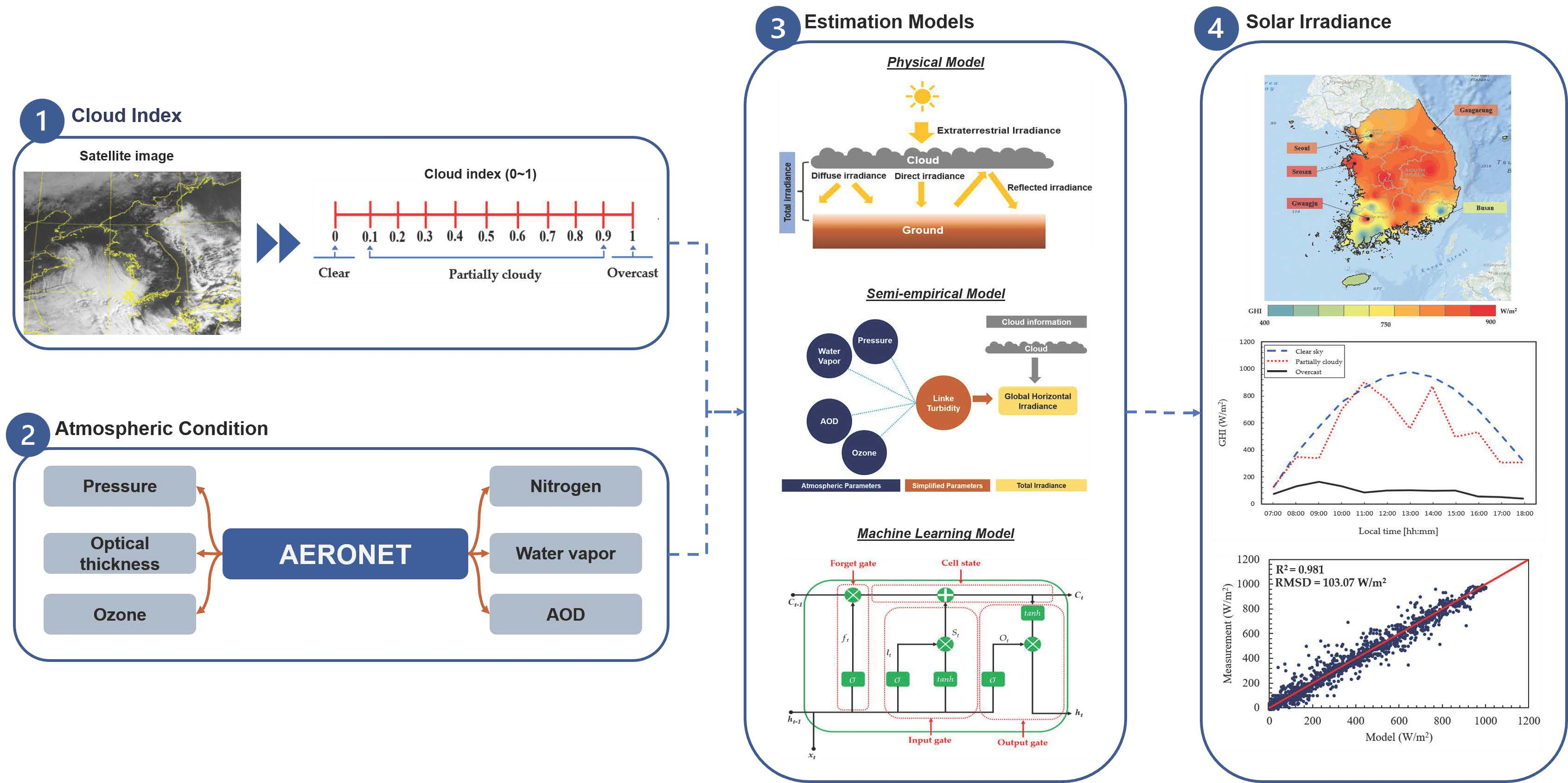
3.1. Cloud Estimation
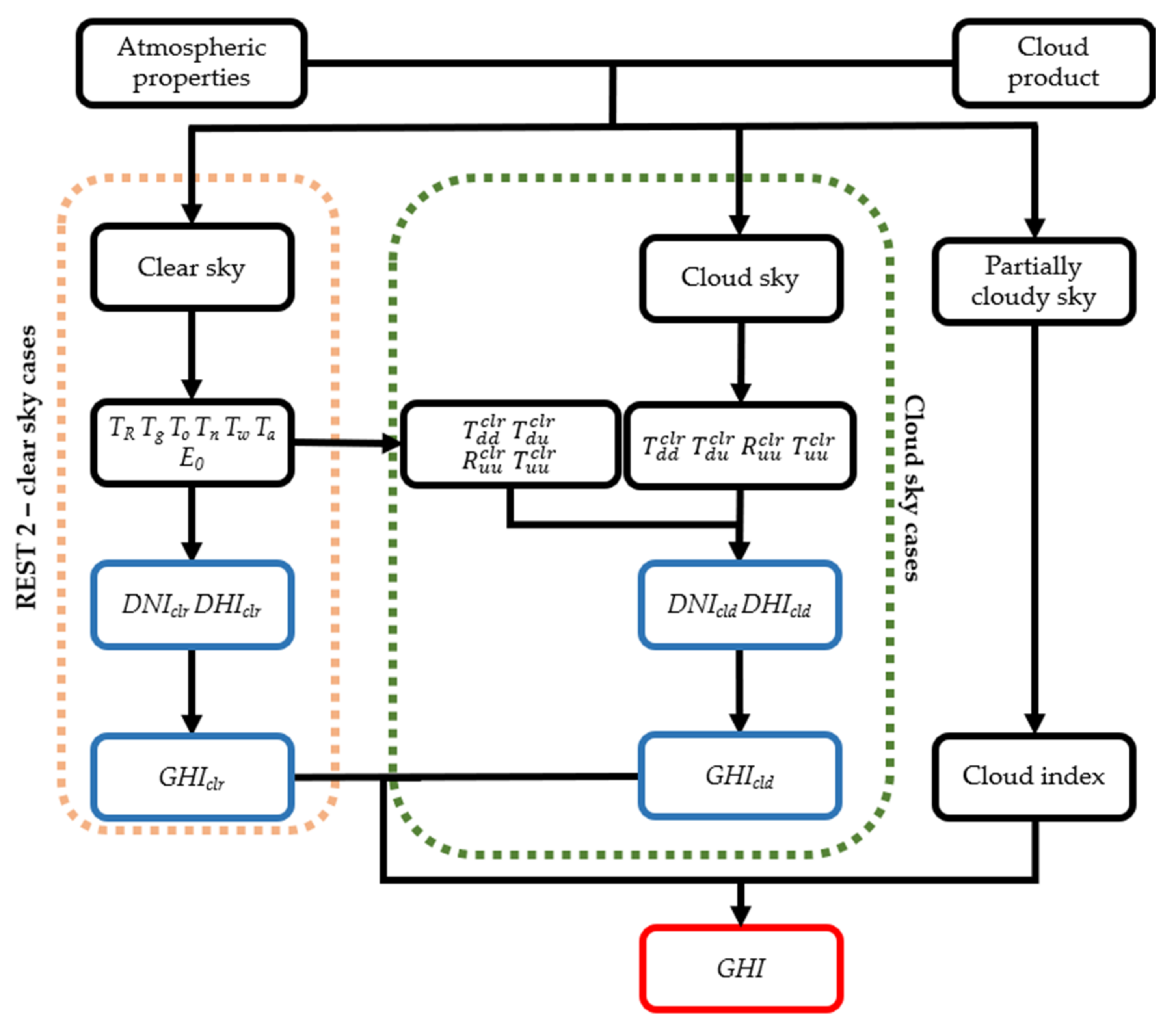
Some agencies, such as KMA, use human observation to scale cloud amounts with an integer value from zero to ten because of its easy practice. Even though this method is convenient, it yields a lot of errors. To reduce these errors, a method to derive cloud conditions was created. This method utilizes an abundant resource of satellite images to select a single pixel and calculates it as a cloud amount, as shown in Figure 2. When sunlight penetrates the atmosphere, clouds are the key factor attenuating solar irradiance. A relative difference in the normalized pixel value between the lower and upper limits of its dynamic range is then used to quantify the amount of cloud. The lower and upper limits correspond to reflectances of the ground and the cloud layer, respectively.
The highest and lowest values of the satellite pixels ( C sat ) are denoted by C max and C min , respectively. The CI value varies from zero to one, with zero indicating the darkest state (clear-sky) and one indicating the brightest condition (overcast).
CI = C sat C min C max C min

3.2. FARMS

It is necessary to calculate both the clear- and cloudy-sky circumstances (denoted by the superscripts clr and cld , respectively) to develop an RT model that can account for solar radiation in all-sky situations. FARMS is based on a solar radiation model with a two-band formulation, where i represents the variable for each band. Each clear-sky direct normal irradiance (DNI) band is derived from the sum of individual transmittances as follows:
DNI clr = T R i T g i T o i T n i T w i T a i T 0 n i μ
where the band transmittances for Rayleigh scattering, evenly mixed gases absorption, ozone ( O 3 ), nitrogen dioxide absorption ( N 2 ), precipitable water ( W P ), and aerosol extinction are T R i , T g i , T o i , T n i , T w i , and T a i , respectfully, and μ is the value of the cosine zenith angle. It also counts the extra-atmospheric irradiances at the mean sun–earth distance, E 0 n i . Note that T R i and T a i were affected by the pressure ( P ), Angstrom coefficient, and turbidity ( α and β ).
For the case of clear-sky diffuse horizontal irradiance (DHI), assuming that the ground is perfectly absorbent (i.e., with zero albedos), the formulation becomes:
E d p i = T o i T g i T w i T n i B R i 1 T R i T a i 0.25 + B a F i T R i 1 T a s i 0.25 E 0 n i μ
where the function F i is a correction factor to compensate for the multiple scattering and B R i is the forward scattering fractions for Rayleigh extinction. Even though the contribution is not significant under normal conditions, a backscattering contribution must be added to get the real interaction between the DHI and the earth’s reflectance. When the scattering effect is added, the formula becomes:
DHI clr = ρ g i ρ s i ( DNI clr + E d p i ) / ( 1 ρ g i ρ s i )
where ρ gi and ρ si are the ground albedo and sky albedo, respectively. Finally, for clear-sky circumstances, total solar irradiance equals the sum of diffuse solar irradiance and direct solar irradiance, as is demonstrated by the following equation:
GHI clr = DNI clr + DHI clr
Figure 3 shows a need for a solar irradiance formulation that is constructed with the premise of considerable cloud accumulation as is required to calculate solar irradiance for all situations fully. In order to calculate this scenario, the direct and diffuse radiation must be separated using two subscript character notations ( d or u ). The character specifies whether the incident radiation is direct (“ d ”) or diffuse (“ u ”) in nature. The second character specifies the state of the outgoing radiation after atmospheric scattering, so “ dd ” signifies incident and outgoing fluxes that are both direct and diffuse, respectively.
The solar irradiance is computed by calculating the transmittance and reflectance of each clear and cloudy condition, as well as the diffuse and direct state of the solar radiation. The transmittance equation is shown below.
T uu clr = 2 0 1 μ T dd clr ( μ )   d μ
T du clr = E d p i E 0 n i
T dd clr = DNI clr E 0 n i
T dd cld = e τ μ
T du cld = s T du , p cld exp log 10 τ τ p 2 D
where T du , p cld and τ P are the maximum of T du cld for each given solar zenith angle and cloud optical thickness as T du cld reaches its maximum, D is a function related to the width of T du cld , and s is a scaling factor that adjusts T du cld when cloud optical thickness is large. The total downward fluxes must be determined to obtain the GHI in these circumstances, so the equation for the first order of total downward flux is as follows:
F 1 = F 0 cos θ z T dd cld T dt clr + T du cld T uu clr
where F 0 denotes the radiative flux at top of the atmosphere. Using the Equation stated above, it is straightforward to calculate the GHI for cloud scenarios using the following equation:
GHI cld = F 1 1 R s R uu clr + R uu cld T uu clr 2 1
where R s is the surface reflectance, R uu clr and R uu cld are the aerosol and cloud reflectance for diffuse fluxes, respectively. Ultimately, using the following function, the cloud index is used to derive GHI under all-sky conditions:
GHI = GHI cld CI + 1 CI GHI clr

3.3. LSTM

The LSTM was proposed as a solution for RNN long-term information incapability. Since the inner cells may carry information unmodified at will, LSTMs can remember information for lengthy periods. The flow of the LSTM is comparable to that of the RNN. However, the network has complete control over the state of the cell, and it may use specific structures (called gates) to add, update, or remove information from the cell. An LSTM unit is made of forget, input, and output gates as shown by Figure 4.
The forget gate determines whether information should be discarded or saved. The input gate changes the state of the cells, and the output gate determines the hidden state. The formula related to the LSTM gates are given as follow:
f t = σ A w f X t + U f h t 1 + b f
i t = σ A w i X t + U i h t 1 + b i
o t = σ A w 0 X t + U o h t 1 + V o C t + b o
where X t is the input vector to the memory cell at time, t and b are bias vectors for every corresponding gates, w and U are weight matrices, and f t , i t , and O t are the values of the input, forget, and output gates. The forget gate ( f t ), input gate ( i t ), and output gate ( O t ) in Equations (14)–(16) have values from 0 to 1 through the sigmoid function ( σ ). A value of 1 indicates that all input data passes through the gate, whereas a value of 0 indicates that no data passes through [47]. An LSTM recognizes the importance of information using backpropagation [48]. The LSTM then uses an internal memory unit to keep important information of the past to boost its performance and further ensure that the vanishing gradient and exploding gradient problems did not occur while training [49]. The formula related to the LSTM memory cell is given as follow:
C t = i t S t + f t S t 1
S t = tanh w c X t + U c h t 1 + b c
h t = O t tan h C t
where S t and C t are the values of the candidate state of the memory cell and the state of the memory cell at time t , respectively, and h t is the value of the memory cell at time t . Equation (17) uses the values of the candidate state of the memory cells to calculate new information at a time t , and the tan h function outputs a value between −1 and 1. The memory state at the cell, controlled by the forget and input gates, is determined as a variable C t of time t according to Equation (16). Then, the specified values are converted to outputs by multiplying them by O t and the output becomes h t , as shown by Equation (19).

3.4. Hammer Model

Using satellite images and Linke turbidity, the Hammer model was developed to estimate GHI (as is shown in Figure 5). A single pixel with an area of 1 km2 is taken from the satellite images, and the pixel brightness defines its value in the range of 0 to 1024. This pixel value is then normalized with the cosine zenith angle, resulting in a geometrically aligned pixel value. This model’s process is visualized in Figure 5.
The C sat is calculated using Equation (20) from the normalized pixel value. Equation (1) can be used to obtain the value of CI after obtaining the value of C sat , with C 0 being the correction factor and C raw as the raw satellite pixel data.
C sat = C raw C 0 I 0 cos θ z ε
With the conversion formula in Equation (21), the CI value is converted into the clearness index k c .
CI 0 . 2   ;   k c = 1 . 2 0 . 2   <   CI 0 . 8   ;   k c = 1     CI 0 . 8 < CI 1 . 1   ;   k c = 2 . 0667     3 . 6667 CI + 1 . 6667 CI 2 1 . 2   <   CI   ;   k c = 0 . 05
The clear-sky model is typically used as the basis for calculating the GHI value in all conditions. The Linke turbidity (accounts for atmospheric conditions) is an essential input parameter in the clear-sky model. The Linke turbidity is also useful for calculating the degree of attenuation owing to absorption and scattering in the atmosphere. In this investigation, the Linke turbidity was calculated using the model developed by Remund et al. [50].
T L = 1 . 8498 + 0 . 2425 W p 0 . 0203 W p 2 + 12 . 427 + 0 . 3153 W p 0 . 0254 W p 2 β
After obtaining the value T L , the values of two of the most important solar irradiance components (DNI and DHI) can now be determined. The Hammer model uses the following formula to find DNI and DHI:
DHI clr = G ext ε 0 . 0065 + 0 . 045 + 0 . 0646 T L cos θ z + 0 . 014 0 . 00326 T L cos 2 θ z
DNI clr = I o ε cos θ z exp 0 . 8662 T L δ R A M
The two components are then added together to form the clear-sky GHI:
GHI clr = DNI clr cos θ z + DHI clr
Finally, the GHI value for all-sky conditions can now be calculated by multiplying the GHI clear-sky and clearness index:
GHI = k c GHI clr

3.5. Model Performance Criteria

In this study, the following metrics were used to calculate the difference rate between the measurements and models. The degree of dispersion of the model against the measurement can be determined using the root mean square difference (RMSD). The overestimation or underestimation of the model against the measurement can be determined using the mean bias difference (MBD). When the RMSD and MBD values are low, the model is regarded as a good model. However, because of the differences between RMSD and MBD, it is tough to claim that a model should be good if only one of them is low. The relative root mean square difference (rRMSD) and relative mean bias difference (rMBD) values were also presented, which can be used to evaluate the accuracies in different cities and models as well as the results from other studies.
RMSD = 1 n i = 1 n P pred P meas 2
rRMSD = 1 n i = 1 n P pred P meas 2 1 n i = 1 n P meas 100 %
MBD = 1 n i = 1 n P pred P meas
rMBD = 1 n i = 1 n P pred P meas 1 n i = 1 n P meas 100 %

4. Result Analysis

The findings were analyzed using multiple metrics with the same dataset, such as data inputs, locations, and accuracy. The results were analyzed in different sections that focused on data inputs, locations, and metrics.
This paper evaluated the performance of the proposed techniques using observed datasets for solar irradiance in Korea. The KMA provided these data sets. The datasets included global sun irradiance measurements with a one-hour resolution for six different locations in Korea over a one-year period. As mentioned, these sites are distributed from the north to the south of Korea, where each site represents a different climate zone.
Figure 6 shows the variability in GHI measurements at all five locations when the sky is clear, partially cloudy, and overcast. The graphs exhibit the highest potential GHI value in each site and the effect of cloud conditions. The scales of 1055.55 W/m2 in Busan at 13:00 on 21 May 2019, and 13.88 W/m2 in Seoul at 18:00 on 27 May 2019, reflect the maximum and minimum values, respectively. Figure 7 shows the distribution of solar irradiance measurement throughout South Korea.
The KMA weather measurement data were used to derive the solar irradiance using the FARMS, Hammer, and LSTM models. Each model flow process was shown in Section 3 and demonstrates how each input influences the output solar irradiance in each model. These inputs are exported to the LSTM as training, validation, and test sets, using the same inputs to generate the FARMS and Hammer models. Table 3 summarizes the input variables utilized in the FARMS, Hammer, and LSTM models.
This part is devoted to examining each model’s output in all the appropriate locations. As each site has its climate, the model’s reliability performance may be determined by comparing the results with other locations using four different metrics. In the original work, the FARMS claims a low RMSD error of approximately 130.28 W/m2 with the selected datasets from 2009 to 2012 [27]. This study confirms that the FARMS performed with an average error of 138.97 W/m2 (the lowest error of 125.34 W/m2 occurred in Seoul and the highest error of 148.75 W/m2 occurred in Seosan). It has a relative RMSD of 32.06% and 33.57%, respectively. This study’s results indicate that FARMS is a fast-processing FARMS with a computation time of roughly 1.02 s and good accuracy even when varied climate conditions are used. The relative error using the Hammer model in every city was tested. The results show that in Korea, the maximum and minimum values of rRMSD were 32.78% in Gwangju and 29.32% in Busan, respectively. This study confirms that this particular method delivers steady and reliable results, as there is not a large gap between the extrema. While the bias error may have a larger value than expected, this is a predictable result since the pixel correction sometimes has extreme error for one or two cases; this can inflate the bias error (as it did in Busan). In most cases, however, it has a value below 10%.
LSTM performs with an R2 above 0.90, as is shown in Figure 8 and Figure 9. However, the best result occurs when LSTM is paired with FARMS, resulting in an R2 of 0.981 in Gangneung. This is the most stable location compared with the other locations. On the other hand, the LSTM–Hammer has a lower correlation, with an R2 of 0.973; this occurred since the Hammer model required C sat as an input, in which the pixel value is subjected to overestimation.
Table 4 is a compilation of the results from each location using four different metrics.
When utilized in temperate, dry winter, and hot summer climates, such as Busan and Seosan, the FARMS is subjected to a significant bias and accuracy error due to the broader range of temperatures throughout the year and more distinct seasonal fluctuations in these locations, which significantly impact pressure and precipitable water. The Hammer model tends to overestimate cities with no dry season. Since the Hammer model simplifies atmospheric conditions, which rely primarily on precipitable water, the estimation becomes less accurate as the value fluctuates, resulting in larger rMBD. The LSTM, unlike the FARMS and the Hammer models, was less affected by the change in climate. Because the LSTM model is based on the correlation of each parameter, it can adapt to the characteristics of various environments.
In Seoul, LSTM using input from FARMS has the lowest rRMSD error compared to other methods, making it the most suitable for that location. Note that LSTM–FARMS has a higher RMSD metric error than LSTM using the Hammer model’s input parameters. This is because Seoul has a cold winter and a dry summer, meaning there is a large gap between the maximum and minimum value of its optical thickness. This could affect the output for LSTM–FARMS, but not for LSTM–Hammer. Hammer’s method does not count optical thickness as a singular input; it counts as one of the Linke turbidity parameters.
When paired with LSTM–FARMS, Gangneung has the lowest error value; however, when utilizing the same method, Gangneung has the greatest value of MBD error compared with the other cities. This is because the method to retrieve the CI value depends on the pixel value of each location since Gangenung is located near the ocean, and the sky is clear most of the time. This resulted in a determination that most CI data were clear-sky data. This is not an issue for the FARMS or Hammer models. However, one cloudy day in Gangenung (even though it is rare) can be overestimated when employing the LSTM, resulting in a greater MBD error. Unlike Gangneung, Seosan has a relatively low bias error but has the highest RMSD of all the locations. This is due to Seosan having a high GHI average compared with the other cities, but has a lower variability between clear-sky, partially cloudy, and overcast cases, as shown in Figure 6. This condition made it easy to overestimate the value of GHI when the sky condition is clear, resulting in a higher average error for this specific location when using both Hammer and FARMS input.
Gwangju has the lowest RMSD error value of all the locations. This was not surprising, as Gwangju has the highest GHI average compared with other locations, making it easier to predict in a clear-sky scenario. It is also easier to see the changes caused by the number of clouds since the value will drastically decrease compared with the normal situation. The lowest value for relative RMSD happens in Busan using the LSTM–FARMS method, as Busan is one of the most stable locations compared with the other cities. This result is strongly correlated to the estimation of this study.

5. Conclusions

Three representatives of physical, semi-empirical, and machine learning models (i.e., FARMS, Hammer, and LSTM) that estimate GHI based on atmospheric and cloud information were evaluated. The models were compared using the same two-year dataset in Korea with hourly measurements from five different locations. This study demonstrated that the LSTM was selected as the most appropriate model for deriving the GHI in Korea in terms of the RMSD and the MBD. Major findings can be summarized as follows.
  • Compared to the Hammer model, the FARMS provides a more precise estimation because the FARMS takes advantage of more detailed information of atmospheric conditions. On the other hand, the Hammer model is more accessible since the input parameters are fewer and commonly measured by an open-access organization.
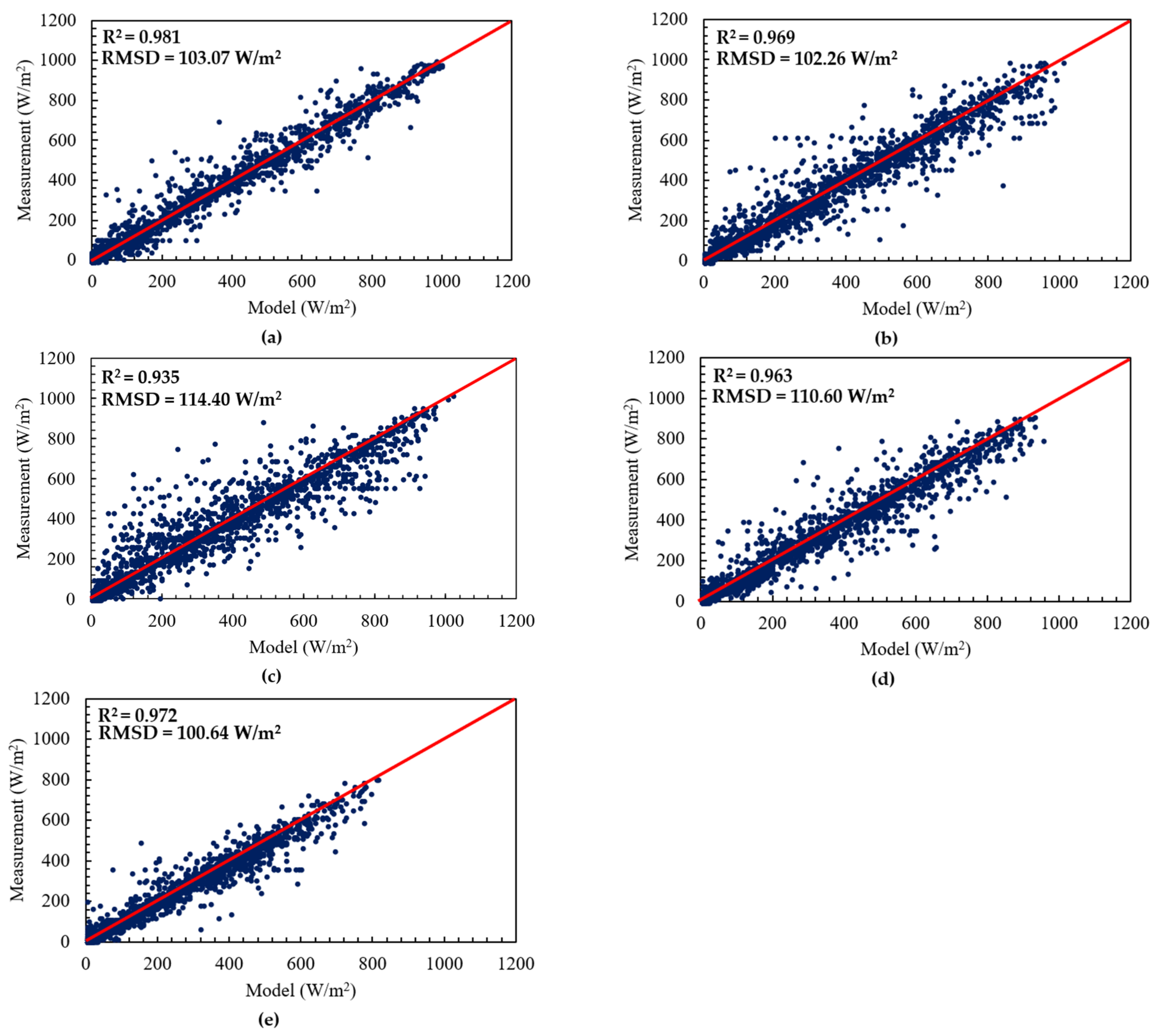
  • In general, the LSTM outperforms the FARMS and the Hammer model in estimating GHI. In comparison to the slight improvement in rRMSD, the improvement in rMBD by the LSTM is significant. The rMBD value less than 1% indicates that long-term means of GHI can be accurately estimated.
  • The LSTM using the FARMS input parameters produces the best accuracy, with a difference in rRMSD of 4.44% compared to its Hammer model counterpart.
  • Based on the climate, the FARMS was subjected to considerable bias and error in locations with a temperate, dry winter, and hot summer climate due to the distinct seasonal fluctuations. On the other hand, the Hammer model tends to overestimate in the cities with no dry season since the value of precipitable water varies. Conversely, the LSTM was primarily unaffected by the change in climate.
This study concludes that the machine learning model performs well regardless of the climate conditions compared to the physical and semi-empirical models. Nevertheless, the advantages of physical and semi-empirical models, such as the lack of training data, ease of implementation, and faster calculation, should also be considered when an estimation model is chosen.

Author Contributions

Conceptualization, R.K., P.M.P.G., H.L.; methodology, R.K.; software and algorithm, R.K.; formal analysis, R.K.; data collection, R.K., P.M.P.G.; review and editing, P.M.P.G., H.L.; funding acquisition, H.L. All authors have read and agreed to the published version of the manuscript.

Funding

This study was financially supported by grants from the National Research Foundation of Korea (NRF), Ministry of Science and ICT (2018M1A3A3A02065823, 2019R1A2C1009501) and the Korea Evaluation Institute of Industrial Technology (KEIT) (20011377) funded by the Ministry of Trade, Industry and Energy.

Institutional Review Board Statement

This research does not involve human or animal.

Informed Consent Statement

This research does not involve humans.

Data Availability Statement

Data are contained within this study.

Conflicts of Interest

The authors declare no conflict of interest.

Nomenclature

A M Air mass
CI Cloud index
C sat Satellite pixel value
C 0 Normalized satellite pixel value
C raw Raw satellite pixel value
G ext Extraterrestrial irradiance
k c Clearness index
P Local pressure, hPa
T Temperature, °C
T L Linke turbidity
O 3 Ozone, atm-cm
OT Optical thickness, cm
N 2 Nitrogen, atm-cm
W P Precipitable water, cm
Greek Symbols
θ back Backscattering angle, deg
θ sat Satellite zenith angle, deg
θ z Solar zenith angle, deg
ε Normalized variation of the sun-to-earth distance from its mean value
ρ Albedo
δ R Rayleigh optical thickness
α Angstrom coefficient
β Angstrom turbidity
Subscripts
clr Clear case
cld Cloudy case
Abbreviations
DHI Diffuse Horizontal Irradiance, W/m2
DNI Direct Normal Irradiance, W/m2
GHI Global Horizontal Irradiance, W/m2
RNN Recurrent Neural Network
LSTM Long Short-Term Memory
MBD Mean Bias Differences (W/m2)
RMSD Root Mean Square Differences (W/m2)
rMBD Relative Mean Bias Differences (%)
rRMSD Relative Root Mean Square Differences (%)
FARMS Fast All-sky Radiation Model for Solar applications
RT Radiative Transfer
KMA Korea Meteorological Administration
COMS Communication, Ocean, and Meteorological Satellite
NASA The National Aeronautics and Space Administration

References

  1. Inman, R.H.; Pedro, H.; Coimbra, C.F. Solar forecasting methods for renewable energy integration. Prog. Energy Combust. Sci. 2013, 39, 535–576. [Google Scholar] [CrossRef]
  2. Duffie, J.A.; Beckman, W.A. (Eds.) Solar Engineering of Thermal Processes, 4th ed.; Wiley: Hoboken, NJ, USA, 2013; ISBN 978-1-118-41541-2. [Google Scholar]
  3. Kleissl, J. Solar Energy Forecasting and Resource Assessment; Elsevier: Amsterdam, The Netherlands, 2013. [Google Scholar] [CrossRef]
  4. Paudel, I.; Cohen, S.; Stanhill, G. The Role of Clouds in Global Radiation Changes Measured in Israel during the Last Sixty Years. Am. J. Clim. Chang. 2019, 8, 61–76. [Google Scholar] [CrossRef] [Green Version]
  5. Lappalainen, K.; Valkealahti, S. Recognition and modelling of irradiance transitions caused by moving clouds. Sol. Energy 2015, 112, 55–67. [Google Scholar] [CrossRef]
  6. Zelenka, A.; Perez, R.; Seals, R.; Renné, D. Effective Accuracy of Satellite-Derived Hourly Irradiances. Theor. Appl. Clim. 1999, 62, 199–207. [Google Scholar] [CrossRef]
  7. Mouhamet, D.; Tommy, A.; Primerose, A.; Laurent, L. Improving the Heliosat-2 method for surface solar irradiation estimation under cloudy sky areas. Sol. Energy 2018, 169, 565–576. [Google Scholar] [CrossRef]
  8. Kim, B.-Y.; Cha, J. Cloud Observation and Cloud Cover Calculation at Nighttime Using the Automatic Cloud Observation System (ACOS) Package. Remote. Sens. 2020, 12, 2314. [Google Scholar] [CrossRef]
  9. Kim, C.K.; Kim, H.-G.; Kang, Y.-H.; Yun, C.-Y. Toward Improved Solar Irradiance Forecasts: Comparison of the Global Horizontal Irradiances Derived from the COMS Satellite Imagery Over the Korean Peninsula. Pure Appl. Geophys. 2017, 174, 2773–2792. [Google Scholar] [CrossRef]
  10. Mommert, M. Cloud Identification from All-sky Camera Data with Machine Learning. Astron. J. 2020, 159, 178. [Google Scholar] [CrossRef]
  11. Huo, J.; Lu, D. Cloud Determination of All-Sky Images under Low-Visibility Conditions. J. Atmos. Ocean. Technol. 2009, 26, 2172–2181. [Google Scholar] [CrossRef]
  12. Wacker, S.; Gröbner, J.; Zysset, C.; Diener, L.; Tzoumanikas, P.; Kazantzidis, A.; Vuilleumier, L.; Stöckli, R.; Nyeki, S.; Kämpfer, N. Cloud observations in Switzerland using hemispherical sky cameras. J. Geophys. Res. Atmos. 2015, 120, 695–707. [Google Scholar] [CrossRef] [Green Version]
  13. Liu, S.; Zhang, L.; Zhang, Z.; Wang, C.; Xiao, B. Automatic Cloud Detection for All-Sky Images Using Superpixel Segmentation. IEEE Geosci. Remote. Sens. Lett. 2014, 12, 354–358. [Google Scholar] [CrossRef]
  14. Kim, B.-Y.; Jee, J.-B.; Zo, I.-S.; Lee, K.-T. Cloud cover retrieved from skyviewer: A validation with human observations. Asia-Pac. J. Atmos. Sci. 2016, 52, 1–10. [Google Scholar] [CrossRef]
  15. Perez, R.; Ineichen, P.; Moore, K.; Kmiecik, M.; Chain, C.; George, R.; Vignola, F. A new operational model for satellite-derived irradiances: Description and validation. Sol. Energy 2002, 73, 307–317. [Google Scholar] [CrossRef] [Green Version]
  16. Sengupta, M.; Xie, Y.; Lopez, A.; Habte, A.; Maclaurin, G.; Shelby, J. The National Solar Radiation Data Base (NSRDB). Renew. Sustain. Energy Rev. 2018, 89, 51–60. [Google Scholar] [CrossRef]
  17. Perez, R.; Seals, R.; Zelenka, A. Comparing satellite remote sensing and ground network measurements for the production of site/time specific irradiance data. Sol. Energy 1997, 60, 89–96. [Google Scholar] [CrossRef]
  18. Sherwood, S.C.; Ingram, W.; Tsushima, Y.; Satoh, M.; Roberts, M.; Vidale, P.L.; O’Gorman, P.A. Relative humidity changes in a warmer climate. J. Geophys. Res. Atmos. 2010, 115, 1–11. [Google Scholar] [CrossRef] [Green Version]
  19. Rubel, F.; Brugger, K.; Haslinger, K.; Auer, I. The climate of the European Alps: Shift of very high resolution Köppen-Geiger climate zones 1800–2100. Meteorol. Z. 2017, 26, 115–125. [Google Scholar] [CrossRef]
  20. Köppen, W. The thermal zones of the Earth according to the duration of hot, moderate and cold periods and to the impact of heat on the organic world. Meteorol. Z. 2011, 20, 351–360. [Google Scholar] [CrossRef]
  21. Kottek, M.; Grieser, J.; Beck, C.; Rudolf, B.; Rubel, F. World Map of the Köppen-Geiger climate classification updated. Meteorol. Z. 2006, 15, 259–263. [Google Scholar] [CrossRef]
  22. Kasten, F.; Czeplak, G. Solar and terrestrial radiation dependent on the amount and type of cloud. Sol. Energy 1980, 24, 177–189. [Google Scholar] [CrossRef]
  23. Qingyuan, Z.; Huang, J.; Siwei, L. Development of Typical Year Weather Data for Chinese Locations. ASHRAE Trans. 2002, 108, 1063–1075. [Google Scholar]
  24. Hu, Y.X.; Stamnes, K. An accurate parameterization of the radiative properties of water clouds suitable for use in climate models. J. Clim. 1993, 6, 728–742. [Google Scholar] [CrossRef] [Green Version]
  25. Mlawer, E.J.; Taubman, S.J.; Brown, P.D.; Iacono, M.J.; Clough, S.A. Radiative transfer for inhomogeneous atmospheres: RRTM, a validated correlated-k model for the longwave. J. Geophys. Res. Space Phys. 1997, 102, 16663–16682. [Google Scholar] [CrossRef] [Green Version]
  26. Berk, A.; Bernstein, L.; Anderson, G.; Acharya, P.; Robertson, D.; Chetwynd, J.; Adler-Golden, S. MODTRAN Cloud and Multiple Scattering Upgrades with Application to AVIRIS. Remote Sens. Environ. 1998, 65, 367–375. [Google Scholar] [CrossRef]
  27. Xie, Y.; Sengupta, M.; Dudhia, J. A Fast All-sky Radiation Model for Solar applications (FARMS): Algorithm and performance evaluation. Sol. Energy 2016, 135, 435–445. [Google Scholar] [CrossRef] [Green Version]
  28. Kim, C.K.; Kim, H.-G.; Kang, Y.-H.; Yun, C.-Y.; Lee, S.-N. Evaluation of Global Horizontal Irradiance Derived from CLAVR-x Model and COMS Imagery Over the Korean Peninsula. New Renew. Energy 2016, 12, 13–20. [Google Scholar] [CrossRef]
  29. Fu, C.-L.; Cheng, H.-Y. Predicting solar irradiance with all-sky image features via regression. Sol. Energy 2013, 97, 537–550. [Google Scholar] [CrossRef]
  30. Hammer, A.; Heinemann, D.; Hoyer, C.; Kuhlemann, R.; Lorenz, E.; Müller, R.; Beyer, H.G. Solar energy assessment using remote sensing technologies. Remote. Sens. Environ. 2003, 86, 423–432. [Google Scholar] [CrossRef]
  31. Rigollier, C.; Lefèvre, M.; Wald, L. The method Heliosat-2 for deriving shortwave solar radiation from satellite images. Sol. Energy 2004, 77, 159–169. [Google Scholar] [CrossRef] [Green Version]
  32. Aslam, M.; Lee, J.-M.; Kim, H.-S.; Lee, S.-J.; Hong, S. Deep Learning Models for Long-Term Solar Radiation Forecasting Considering Microgrid Installation: A Comparative Study. Energies 2019, 13, 147. [Google Scholar] [CrossRef] [Green Version]
  33. Ramadhan, R.A.; Heatubun, Y.R.; Tan, S.F.; Lee, H.-J. Comparison of physical and machine learning models for estimating solar irradiance and photovoltaic power. Renew. Energy 2021, 178, 1006–1019. [Google Scholar] [CrossRef]
  34. Garniwa, P.M.P.; Ramadhan, R.A.A.; Lee, H.-J. Application of Semi-Empirical Models Based on Satellite Images for Estimating Solar Irradiance in Korea. Appl. Sci. 2021, 11, 3445. [Google Scholar] [CrossRef]
  35. Gueymard, C.A.; Ruiz-Arias, J.A. Extensive worldwide validation and climate sensitivity analysis of direct irradiance predictions from 1-min global irradiance. Sol. Energy 2016, 128, 1–30. [Google Scholar] [CrossRef]
  36. Lave, M.; Hayes, W.; Pohl, A.; Hansen, C.W. Evaluation of Global Horizontal Irradiance to Plane-of-Array Irradiance Models at Locations Across the United States. IEEE J. Photovolt. 2015, 5, 597–606. [Google Scholar] [CrossRef]
  37. Komhyr, W.D.; Grass, R.D.; Leonard, R.K. Dobson spectrophotometer 83: A standard for total ozone measurements, 1962–1987. J. Geophys. Res. Space Phys. 1989, 94, 9847–9861. [Google Scholar] [CrossRef]
  38. Mcpeters, R.D.; Bhartia, P.K.; Krueger, A.J.; Herman, J.R.; Wellemeyer, C.G.; Seftor, C.J.; Jaross, G.; Schlesinger, B.M.; Torres, O.; Labow, G.; et al. Earth Probe Total Ozone Mapping Spectrometer (TOMS) Data; NASA Technical Publication: Greenbelt, MD, USA, 1996.
  39. Levelt, P.F.; Van Den Oord, G.H.J.; Dobber, M.R.; Malkki, A.; Visser, H.; De Vries, J.; Stammes, P.; Lundell, J.O.V.; Saari, H. The ozone monitoring instrument. IEEE Trans. Geosci. Remote Sens. 2006, 44, 1093–1101. [Google Scholar] [CrossRef]
  40. Holben, B.; Eck, T.; Slutsker, I.; Tanré, D.; Buis, J.; Setzer, A.; Vermote, E.; Reagan, J.; Kaufman, Y.; Nakajima, T.; et al. AERONET—A Federated Instrument Network and Data Archive for Aerosol Characterization. Remote Sens. Environ. 1998, 66, 1–16. [Google Scholar] [CrossRef]
  41. Holben, B.N.; Tanré, D.; Smirnov, A.; Eck, T.F.; Slutsker, I.; Abuhassan, N.; Newcomb, W.W.; Schafer, J.S.; Chatenet, B.; Lavenu, F.; et al. An emerging ground-based aerosol climatology: Aerosol optical depth from AERONET. J. Geophys. Res. Space Phys. 2001, 106, 12067–12097. [Google Scholar] [CrossRef]
  42. Kasten, F.; Young, A.T. Revised optical air mass tables and approximation formula. Appl. Opt. 2000, 28, 4735–4738. [Google Scholar] [CrossRef] [PubMed]
  43. Wang, X.; Sedlacek, A.J.; DeSá, S.S.; Martin, S.T.; Alexander, M.L.; Alexander, M.L.; Watson, T.B.; Aiken, A.C.; Springston, S.R.; Artaxo, P. Deriving brown carbon from multiwavelength absorption measurements: Method and application to AERONET and Aethalometer observations. Atmos. Chem. Phys. 2016, 16, 12733–12752. [Google Scholar] [CrossRef] [Green Version]
  44. Hochreiter, S.; Schmidhuber, J. Long short-term memory. Neural Comput. 1997, 9, 1735–1780. [Google Scholar] [CrossRef] [PubMed]
  45. Gueymard, C.A. REST2: High-performance solar radiation model for cloudless-sky irradiance, illuminance, and photosynthetically active radiation—Validation with a benchmark dataset. Sol. Energy 2008, 82, 272–285. [Google Scholar] [CrossRef]
  46. Rajagukguk, R.A.; Ramadhan, R.A.; Lee, H.-J. A Review on Deep Learning Models for Forecasting Time Series Data of Solar Irradiance and Photovoltaic Power. Energies 2020, 13, 6623. [Google Scholar] [CrossRef]
  47. Kim, H.Y.; Won, C.H. Forecasting the volatility of stock price index: A hybrid model integrating LSTM with multiple GARCH-type models. Expert Syst. Appl. 2018, 103, 25–37. [Google Scholar] [CrossRef]
  48. Paola, J.D.; Schowengerdt, R.A. A review and analysis of backpropagation neural networks for classification of remotely-sensed multi-spectral imagery. Int. J. Remote Sens. 1995, 16, 3033–3058. [Google Scholar] [CrossRef]
  49. Liu, Y.; Guan, L.; Hou, C.; Han, H.; Liu, Z.; Sun, Y.; Zheng, M. Wind Power Short-Term Prediction Based on LSTM and Discrete Wavelet Transform. Appl. Sci. 2019, 9, 1108. [Google Scholar] [CrossRef] [Green Version]
  50. Remund, J.; Wald, L.; Lefèvre, M.; Ranchin, T.; Page, J. Worldwide Linke Turbidity Information. ISES 2003, 400, 13–26. [Google Scholar] [CrossRef] [Green Version]
Figure 1. South Korea climate classification map based on the work of Wladimir Köppen and Rudolf Geiger.
Energies 14 07939 g001
Figure 2. Process of generating a cloud index from satellite images using pixel normalization.
Energies 14 07939 g002
Figure 3. Procedure to derive solar irradiance using the FARMS architecture with a cloud index.
Energies 14 07939 g003
Figure 4. The structure of a long short-term memory neural network.
Energies 14 07939 g004
Figure 5. The approach of implementing a semi-empirical process using the Hammers model to calculate GHI.
Energies 14 07939 g005
Figure 6. The variability in GHI measurements for clear-sky, partially cloudy, and overcast day: (a) Gangneung (23, 31, and 12 May 2019 for clear, partially cloudy, and overcast); (b) Gwangju (21, 17, and 27 May 2019); (c) Seosan (21, 25, and 27 May 2019); (d) Busan (21, 8, and 27 May 2019); (e) Seoul (2, 20, and 27 May 2019).
Energies 14 07939 g006
Figure 7. Spatial distribution map of South Korea based on global horizontal irradiance measurement data in the year 2018.
Energies 14 07939 g007
Figure 8. Scatterplots of the LSTM-predicted GHI with FARMS input, in which the red curves represent the linear regression fits and the letter indicates the location: (a) Gangneung; (b) Gwangju; (c) Seosan; (d) Busan; (e) Seoul.
Energies 14 07939 g008
Figure 9. Scatterplots of the LSTM-predicted GHI with Hammer input, in which the red curves represent the linear regression fits and the letter indicates the location: (a) Gangneung; (b) Gwangju; (c) Seosan; (d) Busan; (e) Seoul.
Energies 14 07939 g009
Table 1. Summary of the physical, semi-empirical, and machine learning models to estimate solar irradiance.
ReferenceYearAreaKöppen–Geiger ClassificationNumber of LocationsModelRMSD (W/m2)rRMSD
(%)
Xie et al. [27]2016United StatesTemperate (Cfa)1Physical130-
Kim et al. [28]2016KoreaContinental (Dwa)4Physical14657
Fu et al. [29]2016AsiaTemperate (Cfa)1Physical169-
Hammer et al. [30]2003EuropeTemperate (Cfa Cfb, Cfc, Csa, Csb)
Continental (Dfa, Dfb)
1Semi-empirical-35
Perez et al. [15]2002United StatesTemperate (All subtypes)
Continental (All subtypes)
10Semi-empirical118-
Rigollier et al. [31]2004EuropeTemperate (Cfa, Cfb, Cfc, Csa, Csb)
Continental (Dfa, Dfb)
35Semi-empirical-45
Aslam et al. [32]2019KoreaTemperate (Cwa)2Machine learning113-
Ramadhan et al. [33]2021KoreaTemperate (Cwa)1Machine learning10226
Garniwa et al. [34]2021KoreaTemperate (Cwa)1Machine learning7621
Table 2. Measurement locations based on the Köppen–Geiger climate classification.
Station NameLocationsKöppen-Geiger Climate
Seoul37.4580° N, 126.9511° ECold, dry winter, hot summer (Dwa)
Gangneung37.7710° N, 128.8670° ECold, no dry season, hot summer (Dfa)
Gwangju35.2282° N, 126.8431° ETemperate, no dry season, hot summer (Cfa)
Seosan36.5385° N, 126.3301° ETemperate, dry winter, hot summer (Cwa)
Busan37.3388° N, 127.2658° ETemperate, dry winter, hot summer (Cwa)
Table 3. Summary of the data input for the GHI models.
ModelData Input
FARMS CI , P , OT , O 3 , N 2 , W p , θ z , α , β
Hammer C sat , T L , θ z , θ sat , θ back
LSTM-FARMS CI , P , OT , O 3 , N 2 , W p , θ z , α , β
LSTM-Hammer C sat , T L , θ z , θ sat , θ back
Table 4. FARMS, Hammer, and LSTM for estimating the GHI model in each location.
LocationModelRMSD (W/m2)rRMSD (%)MBD (W/m2)rMBD (%)
SeoulFARMS125.3432.0618.144.64
LSTM-FARMS100.6425.740.540.14
Hammer119.6530.6134.288.77
LSTM-Hammer114.3929.269.852.52
GangneungFARMS134.2331.5711.952.81
LSTM-FARMS103.0724.242.380.56
Hammer136.1432.0236.228.52
LSTM-Hammer121.8528.669.692.28
SeosanFARMS148.7533.574.531.02
LSTM-FARMS114.4025.821.460.33
Hammer138.6431.2918.874.26
LSTM-Hammer124.2928.052.530.57
GwangjuFARMS140.1932.5213.583.15
LSTM-FARMS102.2623.723.840.89
Hammer141.2932.7837.808.77
LSTM-Hammer123.3328.617.551.75
BusanFARMS146.3732.7832.827.35
LSTM-FARMS110.6024.775.491.23
Hammer130.9129.3232.687.32
LSTM-Hammer130.4329.214.551.02
Publisher’s Note: MDPI stays neutral with regard to jurisdictional claims in published maps and institutional affiliations.

