Article

Analysis of the Influence of DTM Source Data on the LS Factors of the Soil Water Erosion Model Values with the Use of GIS Technology

by
Anna Fijałkowska
Department of Photogrammetry, Remote Sensing and Spatial Information Systems, Warsaw University of Technology, Pl. Politechniki, 100-661 Warsaw, Poland
Remote Sens. 2021, 13(4), 678; https://doi.org/10.3390/rs13040678
Submission received: 31 December 2020 / Revised: 29 January 2021 / Accepted: 9 February 2021 / Published: 13 February 2021
(This article belongs to the Special Issue Remote Sensing of Soil Erosion)

Abstract

:
Counteracting soil degradation is one of the strategic priorities for sustainable development. One of the most important current challenges is effective management of available resources. Multiple studies in various aspects of soil water erosion are conducted in many research institutions in the world. They concern, among others, the development of risk estimation models and the use of new data for modelling. The aim of the presented research was a discussion on the impact of the accuracy and detail of elevation data sources on the results of soil water erosion topographic factors modelling. Elevation data for this research were chosen to reflect various technologies of data acquisition, differences in the accuracy and detail of field forms mapping and, consequently, the spatial resolution of the digital terrain models (DTMs). The methodology of the universal soil loss equation USLE/RUSLE was used for the L and S factors modelling and calculation. The research was carried out in three study areas located in different types of geographical regions in Poland: uplands, highlands and lake districts. The proposed methodology consisted of conducting detailed comparative elevation and slope value assessments, calculating the values of topographical factors of the universal soil loss equation: slope length (L) and slope (S) and a detailed analysis of the total LS factors values. An approach to assess LS factors values within homogeneous areas such as agricultural plots has also been proposed. The studies draw the conclusion that the values of topographical factors obtained from various DTM sources were significantly different. It was shown that the choice of the right modelling data has a significant impact on the L and S factors values and, thus, also, on the decision-making process. The conducted research has definitely shown that data of the highest accuracy and detail should be used to study local phenomena (inter alia erosion), even analysing a large area.

Graphical Abstract

1. Introduction

Soils are the basis for plant production and food security. The 2015 Food and Agriculture Organization (FAO) report “Status of the World’s Soil Resources” began with the statement: “Soils are fundamental to life on Earth” [1]. In paragraph 10, The Updated FAO World Soil Charter of 2015 emphasised that soil degradation significantly reduces or even eliminates the natural functions of soil. Preventing or minimising soil degradation is necessary to maintain basic functions of soils and is much more economically viable than the reclamation of degraded soils [2,3]. Unfortunately, it is estimated that most of the world’s soil resources are in merely adequate, poor or very poor conditions, and 33% of the land is moderately-to-severely degraded due to, among others, water, wind and crop erosion. It is predicted that a further loss of soil productivity threatens the balance and security of food production, which will cause further price increases and potentially worsen the quality of life of millions of people [2].
In 1983, Renard and Foster, working on a mathematical description of the factors causing water erosion, proposed a general formula showing the dependence of the extent of soil loss on the factors that cause it [4]. Since then, various approaches to erosion modelling have been developed (expert-based [5,6], conceptual, empirical [7,8,9] and physics-based/mechanistic models [7,10]), and these different models have different versions that have undergone many changes and improvements as research has developed [11]. Empirical models constitute an important group of erosion models. These formulas are developed on the basis of the results of research conducted on experimental plots. It is estimated that, for calibrating empirical models of water erosion, we currently have results from over 24,000 measurements conducted mainly in the USA, Europe, Brazil and China [12]. Unfortunately, they are often impossible to compare due to the large diversity of climatic zones and the characteristics of individual slopes [7,8,9,13,14]. Measurements on experimental plots of a given size and with an area limited by natural terrain barriers are not able to adequately reflect the dynamics of the erosion process. During each erosion event, the distance of displacement of the eroded soil material may be different [14]. Moreover, this type of research requires significant financial outlays and is time-consuming, and the obtained results often cannot be extrapolated to larger areas [7,9,15,16]. Despite the above-mentioned limitations, the ease of implementation of empirical equations and the availability of data make these models one of the most popular methods used to assess the impact of water erosion.
The most widely used model in the empirical model range is the Universal Soil Loss Equation, developed in 1965 [17] and its modifications presented in many later studies. The formula for calculating the average annual soil loss is presented in Equation (1):
A= R * K * C * L * S * P
where:
  • A = mean annual soil loss (in t ha−1 yr−1),
  • R = rainfall erosivity factor (in MJ mm ha−1 h−1 yr−1),
  • K = soil erodibility factor (in t h MJ−1 mm−1),
  • C = cover management factor (dimensionless),
  • L = slope length factor (dimensionless),
  • S = slope steepness factor (dimensionless) and
  • P = support practice factor (dimensionless).
Models based on the universal soil loss equation USLE/RUSLE methodology [18] are commonly used to estimate the risk of soil water erosion in analyses covering small areas (single farmland and slopes), as well as in analyses for large areas (one or more catchments). Some of the research conducted was undertaken by [19,20,21,22,23,24,25,26,27,28,29,30,31,32,33,34,35,36,37,38,39,40,41,42,43,44,45,46,47,48]. The European Soil Data Centre (ESDAC) and the European Soil Bureau (JRC) also use these equations when calculating soil loss, including in the PESERA, G2 and RUSLE2015 models [42]. Various authors have emphasised the importance of proper determination of the impact of each factor included in a given erosion model: the precipitation [25,49], the natural susceptibility of soils to erosion [22,50] and land cover and land use [42,50,51], but the vast majority indicate that the factors of length (L) and slope (S) are those whose precise calculations determine the obtained results to the greatest extent. Additionally, uncertainty analyses indicate the significance of these factors [19,22,29,36,37,42,49,50,51,52,53,54,55,56,57].
The models mentioned above differ, inter alia, in the formulas that are used to calculate the impacts of individual factors. In determining the impact of the topography, the most common calculation of the L factor value is based on the distance travelled by the runoff water or on the basis of the unit upslope contributing area, understood as the area from which the water flows to a given point [19] (considered to better reflect the erosive impact of the track passed by water flowing down the slope than a simple linear flow path). The determination of unit upslope contributing areas involves the identification of flow directions for this purpose and the calculation of flow accumulation on its basis. Algorithms that can be used to determine the paths of water flowing down the slope is the assumption of water runoff from the higher raster cells to only one cell (single flow) or to several lower cells (multiple flow). The most frequently used single-flow algorithms are D8, Rho8 and KRA, while the multiple flow algorithms include, among others, DF8, FRho8, D∞, MD∞ and DEMON [37,58]. Despite the expected accuracy of the obtained results, the tests of the above-mentioned algorithms do not always yield similar results, which is often caused by the complexity of the terrain being analysed [59]. Some authors emphasise a much better efficiency of the DEMON algorithm or divergent runoff models [23,37,60], while others indicate no significant differences in the course of the hydrographic network determination and the value of the runoff accumulation [61,62]. The common use of the USLE/RUSLE models facilitates a comparison of the obtained results. A review of the literature sources showed that various data are used to calculate water erosion soil losses and to indicate areas particularly exposed to it (so-called “hot spots”). It can be seen that the obtained results were sometimes significantly different. This is confirmed by the comparison (review) of the selected results of European studies presented in Table 1.
The analysis of the above list led to the following questions: why are there such differences in the obtained results (maximum soil loss values vary from 6.4 t ha−1 y−1 to 11,680 t ha−1 y−1, while research at the pan-European level reaches little more than 50 t ha−1 y−1)? Where do they come from? What causes such discrepancies? Which factors contribute to such differences? If it is the influence of the length and gradient of the slope, do the obtained differences result from the digital terrain model (DTM) source data, their resolution, the formula used or its implementation in a software used?
The literature review gives the impression that, usually, a widely available data is used without first considering the appropriate accuracy and detail of the source data and their impact on the modelling results. Very often, a medium-scale DTM is used to model a phenomenon that is clearly local in nature. This approach is understandable for analyses performed in the absence of available data of adequate detail and accuracy, but it raises doubts in times of the widespread availability of high-resolution elevation data. Although the term “high-resolution DTM” has significantly changed its meaning since the inception of Geographical Information System (GIS) technology, many authors dealing with soil water erosion indicate that the use of source data with high accuracy and detail is an essential aspect of erosion modelling [34,37,55,83,84,85]. Moreover, some studies concerning the uncertainty of the model results indicate that the uncertainty of estimating the values of the L and S factors is crucial. This impact can be reduced by using DTM with very high accuracy and detail [11,39,52,85,86,87,88]. Initially, the data sources for calculating the values of the L and S factors came from field studies; then, they were obtained by vectorisation of the base of topographic maps in different scales [39] and, then, from DTM from various sources (active and passive satellite data [38,56], aerial photography or laser scanning [85,89,90]). The spatial resolution of DTM varied from 0.25 m [91] to 90 m, including data from the SRTM mission [32,35] DTED Level 2 [32,92] EU-DEM model (SRTM update based on ASTER GDEM) [42], as well as models from aerial photos and ALS [85,89,90]. For individual fields, GNSS measurements were also made in a regular grid [60]. In the project implemented for the entire EU area, the values of the L and S factors were calculated from the EU-DEM model (SRTM + ASTER) with a spatial resolution of 25 m, as it is the highest spatial resolution of a homogeneous DTM available for all of Europe. Individual Member States have used DTM with a resolution of 10–40 m to model the risk of water erosion [93].
However, the sensitivity of the erosion models to the source data used has not been comprehensively investigated so far, although the publications emphasise the impact of the accuracy and detail of the source DTM on the values of the L and S factors obtained as a result of its processing [39,43,94]. Tests evaluating the effect of reducing the spatial resolution of source DTM on the modelling results were conducted by, among others, Molnar and Julien [95], Wilson [58], Lee and Lee [88], Liu et al. [96] and Zhao et al. [83].
The methodology used by these researchers assumed the study of the dependence of the obtained results on the spatial resolution of DTM and the subsequent versions of the original DTM, with increasingly lower resolutions (obtained as a result of degradation of the source data resolution). Such models are consistent and only simulate the real data with lower resolutions. However, such comparisons did not make possible the check of the impact of the real data source on the erosion modelling (e.g., possible shifts of terrain forms, lack of visibility of minor terrain forms; this problem is well-reflected in comparative analyses of the hydrographic network system and catchment boundaries obtained from DTM from various sources). Taking into account the high availability of various elevation data for the area of the country or even on a continental scale (obtained with the use of different technologies and characterised by different accuracies and details). There is a need to conduct in-depth research aimed at determining the impact of the source of elevation data on the results of determining the values of the L and S factors of soil water erosion modelling and, consequently, on the determination of areas at risk of water erosion.

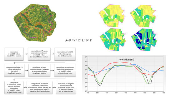
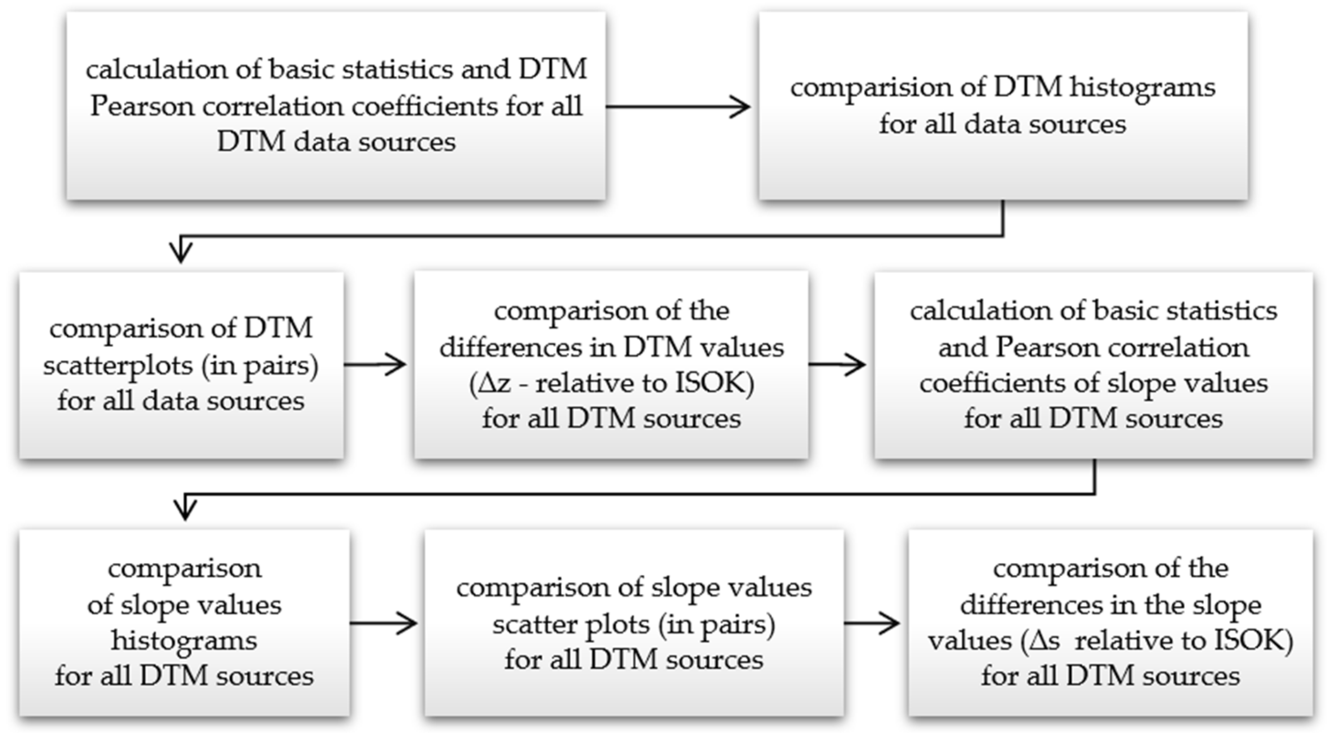
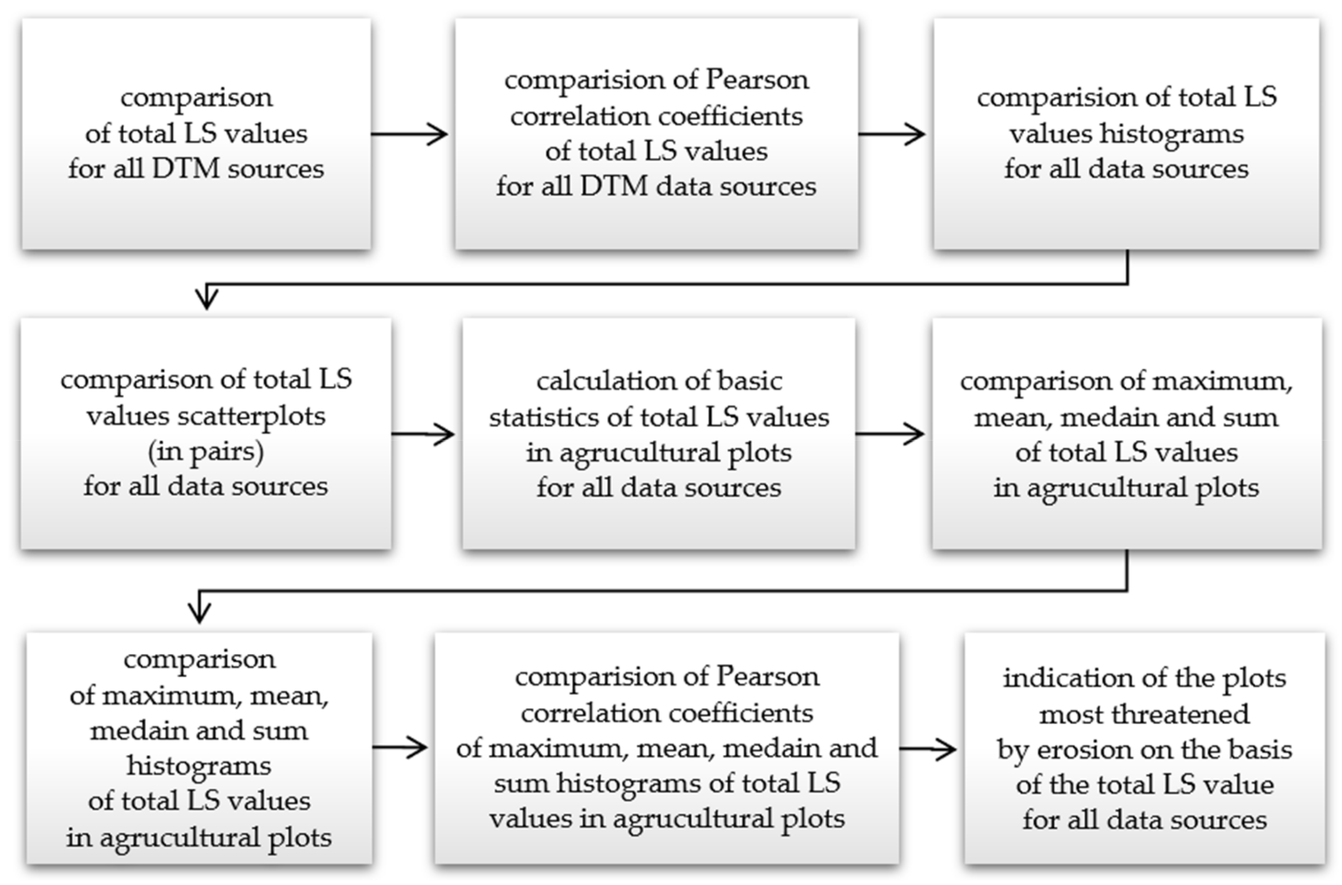
2. Materials and Methods
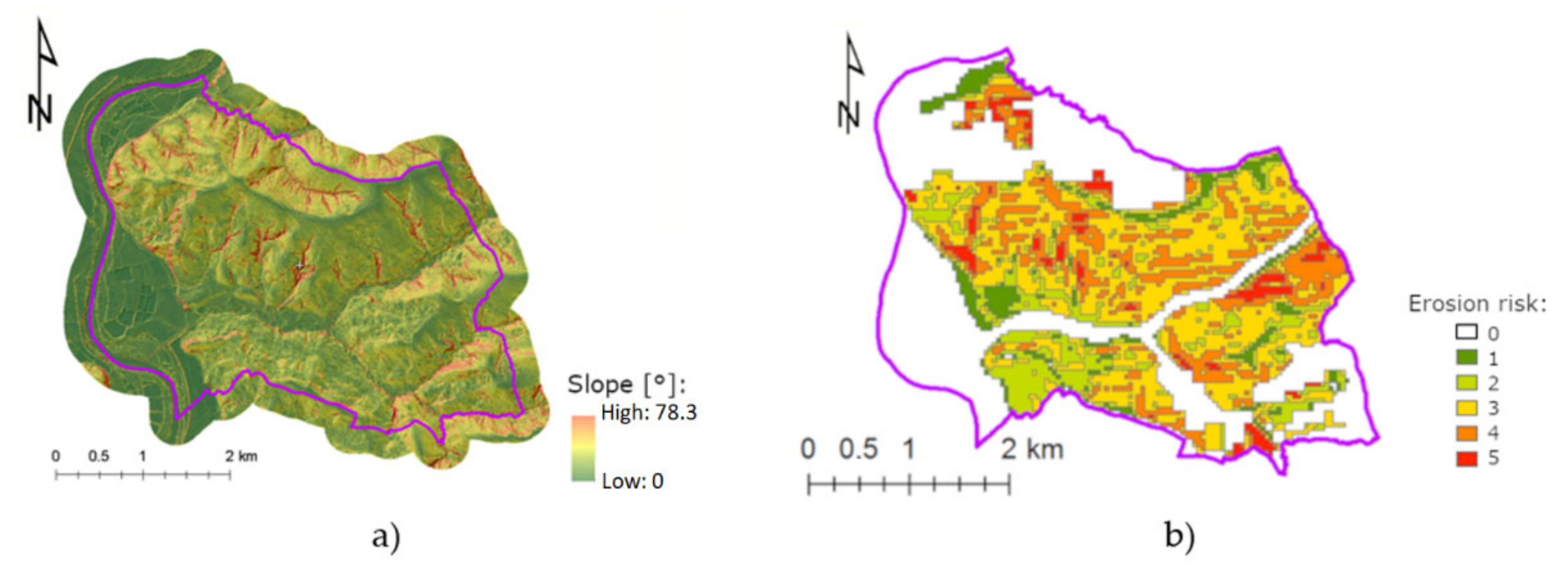
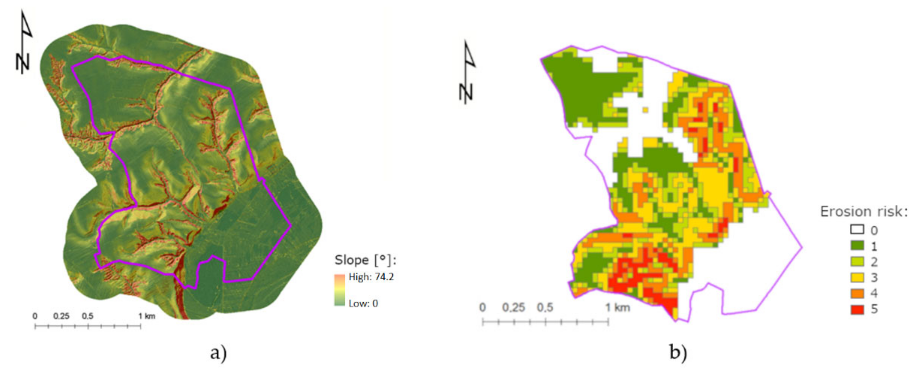
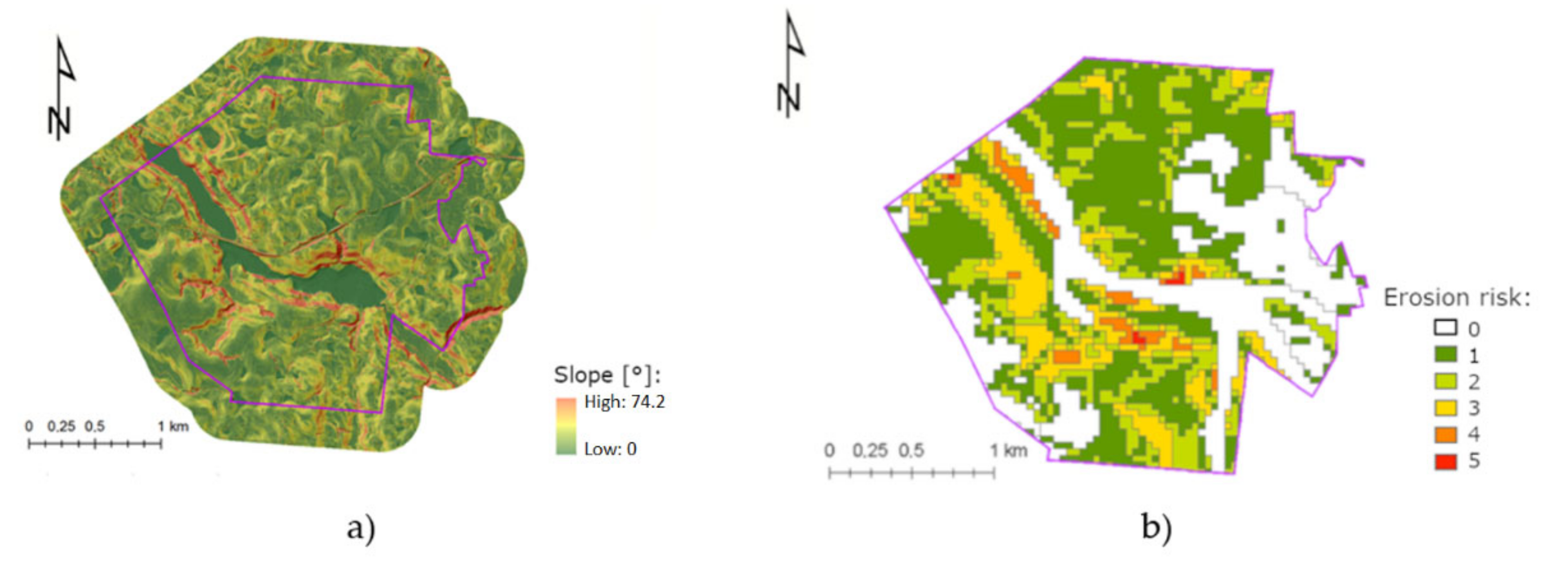
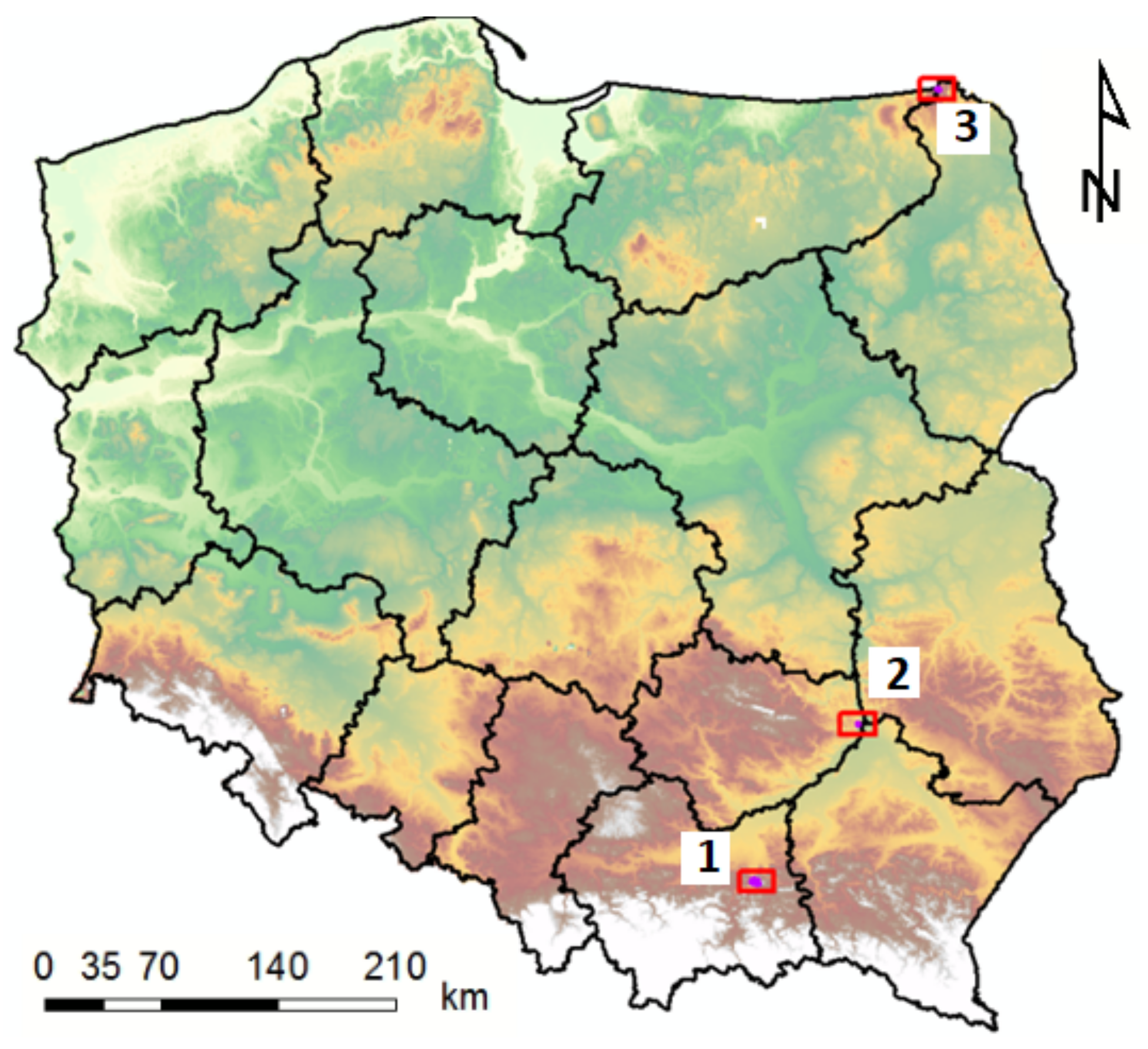
2.1. Study Areas

The proposed methodology was applied in 3 research areas, the selection of which was preceded by an analysis of data available for Poland describing the risk of water erosion developed by The Institute of Soil Science and Plant Cultivation (IUNG). The water erosion risk database distinguishes 6 levels (an expert classification based on: slope class, soil texture classes and total annual rainfall class) of erosion risk: from 0—no risk to 5—very strong erosion risk (dimensionless). The research areas are characterised by varied topography and were selected in such a way that they contain areas of high erosion risk: levels 4 and 5, as well as areas with no risk and low erosion risk: levels 0 and 1. The research areas are located in various types of physical and geographical regions of Poland: foothills, highlands and lake districts (Figure 1).
The research area of Janowice covers an area of 1355 ha and is located in the Western part of Pogórze Ciężkowickie. The terrain heights (based on ALS data) range from 199 m above sea level up to 454 m above sea level. The maximum slopes of the terrain are significant and reach values up to 78° (ALS data) (Figure 2a).The land is mainly covered by grasslands and agricultural crops (55.9%), forests and wooded areas (29.3%), built-up areas (5.8%) and permanent crops (4.5%) (based on the BDOT10k topo reference database).
The research area of Winiarki covers an area of 277 ha and is located in the eastern part of the Sandomierz Upland. Terrain heights (ALS data) range from 138 m above sea level up to 208 m above sea level, and the slope values (ALS data) in this area reach 74° (Figure 3a). The land is mainly covered by permanent crops (38.1%), grasslands and agricultural crops (32.5%), forests and wooded areas (23.3%) and built-up areas (5.5%) (based on the BDOT10k topo reference database).
The research area of Bolcie covers an area of 501 ha and is located in the northern part of the East Suwałki Lake District. The north-western part of the area border coincides with the Polish and Lithuanian borders. The terrain altitudes (ALS data) vary from 206 m above sea level up to 273 m above sea level. The slope values in this area (ALS data) reach up to 59° (Figure 4a). The land is mainly covered by grasslands and agricultural crops (89.9%), forests and wooded areas (5.8%), water bodies (3.0%) and built-up areas (1.1%) (based on the BDOT10k topo reference database).
As already mentioned, the selection of research areas was preceded by an analysis of the water erosion risk in these areas (Figure 2b, Figure 3b and Figure 4b).

2.2. DTM Source Data

At present, a wide range of DTM and digital surface model (DSM) data is available nationwide (homogeneous data for the territory of Poland). These data were created as a result of the use of various technologies; therefore, they are characterised by varying accuracies and details of mapping the terrain forms, varying spatial resolutions resulting from these parameters, as well as varying validities. The list of the most frequently used data sources is presented in Table 2.
As a result of the review and analysis of the above-described sources of elevation data, the following data were selected to test the sensitivity of the soil water erosion model: SRTM, DTED2, LPIS and ISOK.
The DTED2 DTM was developed by the vectorisation of contour lines from military topographic map diapositives with the scale of 1:50,000. The spatial resolution of the raster data was 25 m/30 m. Many tests performed showed that these data are usually of better quality than indicated by the nominal data metric (nominal absolute error in determining the height of points can be up to 26 m). In experimental work carried out at the Warsaw University of Technology, it was estimated that the accuracy of the height determination for the areas around Warsaw is 2 to 3 m.
The LPIS DTM is mainly used to generate orthophotomaps for ARMA (Agency for Restructuring and Modernisation of Agriculture). Aerial photos in the scale of 1:26,000 and topographic maps of 1:10,000 for inaccessible (mainly forest) areas were used for its construction, and new data was obtained in accordance with the data update ARMA schedule. This model has a height accuracy of 1 m–1.5 m. It is possible to obtain free-of-charge data from The National Geodesy and Cartographic Resources (PZGiK). It is recommended to generate raster DTM with 10-m spatial resolution from the LPIS source data.
In 2010, the implementation of the ISOK project aimed at preventing crises in flood zones was started in Poland. As part of the project, point clouds in the technology of airborne laser scanning (ALS) were obtained. The source measurement data are stored in the form of a classified point clouds with a density depending on the degree of land use from 4 points/m2 (standard I) to 12 points/m2 (standard II). As a rule, the data in standard I should meet the accuracy assumptions of the mean error of the x and y coordinates: mx, y < 0.5 m and the z coordinate: mz < 0.15 m, while the data in standard II should meet the accuracy assumptions of the mean error of the x and y coordinates: mx, y < 0.4 m and the z coordinate: mz < 0.10 m [101]. Measurement data, as well as the raster forms of DTM and DSM, can be obtained free-of-charge from the PZGiK resource. It is recommended to generate raster DTM from the ISOK source data with 0.5-m or 1-m spatial resolution, depending on the standard (II or I). This resolution is sufficient to reflect the relief of the terrain with sufficient detail for hydrological studies [90].
The elevation source data was selected so that, in the raster form, they present the sequence of spatial resolution: from 90 m to 1 m (resulting from the accuracy and detail of the source data), as well as different techniques of data acquisition and different ones up-to-date. The selected DTMs were acquired on the following dates: SRTM (2000), DTED2 (1980), LPIS (05.2008–06.2009) and ISOK (10.2011–04.2012). Due to the fact that the analysis carried out in this project concerned agriculture areas, the problem of the different validities of the data and model types (DTM/DSM) was considered negligible. All DTM data were preprocessed (e.g., sinks filling or raster snapping) for being as suitable as possible for further analysis.

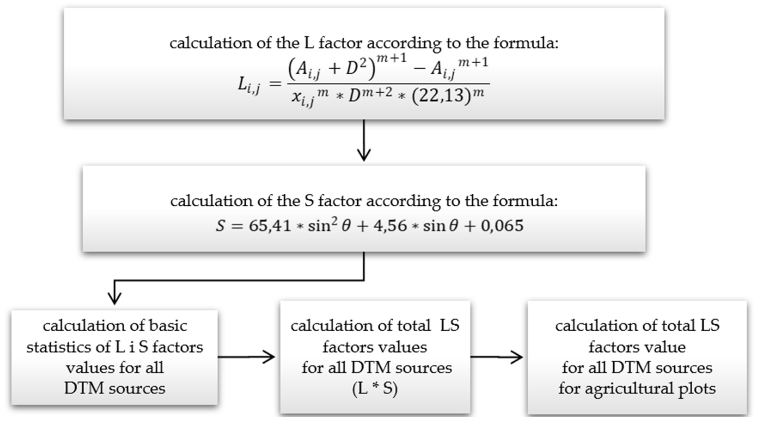
2.3. USLE/RUSLE LS Formulas Implementation

As mentioned in the introduction, few authors have attempted to compare the results of water erosion modelling by testing various data sources for individual criteria. The most frequently used methodologies assume either the study of a new data source or introduction of new approaches to determining the value of one of the factors or the entire model by comparing the obtained new results with the results obtained on the basis of previously used data or technologies [38,42,43,102,103,104,105] or comparing these with the results obtained using the methodology used so far [17,19,30,36,48,55,106].
The examples of assessing the influence of spatial resolutions of the DTM on the values of DTM derivatives, including the values of the L and S USLE/RUSLE factors [58,88,95,96] found in the literature review, assumed performing tests with the use of a single DTM source with increasingly lower resolutions, obtained by degrading the resolution of the original DTM of high spatial resolution as an adopted methodology. On the other hand, this project assumed the use of various original data sources available for the territory of Poland, which differ in both spatial resolution (resulting from the accuracy and detail of the source data) and the technology of the data acquisition. Initial data processing showed that, despite the similarity of the elevation values, the values of DTM derivatives differ significantly between individual datasets. Therefore, the presented methodology includes not only an analysis of the value of the L and S factors obtained from different source data but, also, a comparative analysis of the DTM values and the values of the land slopes.
For this reason, the proposed methodology consists of the following steps:
• stage 1
determination of the mask of agricultural areas inside the research areas (exclusion of nonagricultural part from statistics calculation),
• stage 2
detailed comparative analyses of elevation values and slope values obtained from various DTM source data,
• stage 3
calculation of the values of the L and S factors in accordance with the adopted formulas and with use of various DTM source data and
• stage 4
detailed analyses of the total value of the LS factors obtained from different DTM source data.
The values of basic statistics (minimum, maximum, arithmetic mean, standard deviation, median and range) were used to compare the values of elevation, slopes and LS factors.
The first step (stage 1) was to determine the mask of agricultural areas within the boundaries of the research areas. Although the calculation of the values of the L and S factors was performed for the entire studied areas, the comparison of the obtained values was carried out only within the area of agricultural use. This is supported by the fact that water erosion is primarily a threat to arable soils, and the research conducted mainly focused on predicting and preventing erosion in these areas. The second premise results from the previously mentioned specificity of the data used. SRTM data is defined as a digital surface model (DSM), and that is why comparing its derivatives with derivatives obtained from other DTM sources in wooded areas carries the risk of obtaining different processing results. This mask was developed on the basis of data provided by ARMA.
All statistics for DTM data and their derivatives were developed to facilitate a possibility of comparing the obtained results on the basis of the values assigned to points (vector layer) distributed within the study areas in a regular grid of 1 m × 1 m. Thus, for the results obtained from all DTM sources, the number of observations in each research area is the same. Moreover, this approach guarantees a comparison of the values obtained in exactly the same locations.
The methodology of the comparative analysis of DTM (after preprocessing, e.g., sink filling) and slopes values (stage 2) is presented in Figure 5.
The next stage (stage 3) of the study was the calculation of the values of the L factor and the S factor depending on the DTM data source used for the calculations, as well as comparison of the obtained values. An indication of the formulas used and the subsequent analysis included in this stage are presented in Figure 6.
When determining the influence of the L and S factors on the water erosion estimation, many authors, referring to the USLE/RUSLE methodology, do not always carry out calculations according to the same assumptions and formulas. The choice of the formulas described by the equations presented in the scheme for the implementation of this stage (Figure 6) was based on the assumption that the equations should contain as few fixed values and simplifications as possible (e.g., assuming a specific value of one of the parameters for a specific range of slopes). These formulas were also selected by researchers from the Joint Research Centre (JRC)—European Soil Data Centre (ESDAC) [26,29,32,35,41,43,68,92]. The RUSLE2015 project to designate the areas of water erosion risk for EU countries also used them [40,42]. In this study, the simplest single-flow algorithm (D8) was used to calculate the unit slope contribution areas to minimise the impact of the division of the runoff paths or a random factor on the calculation results.
The next stage (stage 4) of the performed analysis consisted of an in-depth analysis of the value of the total impact of the L and S factors, calculated as the multiplication of their values (LS) (Figure 7).
Then, the total LS value threshold for 95% and 99% of the pixels were determined and compared with the maximum values of each of the datasets. The threshold values are understood to be the limit values within which 95% and 99% of the agricultural land in each research area falls, respectively. The significant difference in the value between the threshold value and the maximum value for research indicates the presence of small areas with very high values of the total LS factor values, interpreted as an indicator of the places most exposed to erosion due to their topography.
In the next step of stage 4, the calculated LS values from DTMs with lower resolutions were compared to the LS value calculated from ISOK. The Pearson correlation coefficients were calculated for all pairs of results and the scatter plots for the least and most correlated pairs of the total LS factors values analysed. At the end of this stage, the following statistical values relating to the area of the entire agricultural plot were calculated: the sum, standard deviation, mean, median and the maximum of the total LS factors value.
The comparison of the total LS factors values calculated from ISOK and other DTM sources in agricultural plots was carried out by calculating the value of the variability index WZ (Equation (2)). This indicator shows what effect the calculation of the total LS factors values with DTMs of lower accuracy and detail would have on the final value obtained from the USLE/RUSLE equation. The lowest values (close to 0) indicate a significant underestimation of the total LS factors values relative to ISOK, while very high values, a significant overestimation of the value of the total LS factors values relative to ISOK. The values of the WZ variation index ranging from 0.9 to 1.1 (±10%) were considered to be the values comparable to those obtained from ISOK.
W z = L S S U M   i L S S U M   I S O K
where:
  • LS SUM i: the total value of LS factors obtained for the agricultural plot based on SRTM, DTED2 and LPIS;
  • LS SUM ISOK: the total value of LS factors obtained for the agricultural plot based on ISOK.
The analysis that complements the described calculations is the visualisation of the DTM elevation value, land slopes and the total LS factors values along the selected terrain profiles. Localisations of the profiles were selected so that they pass through areas with a significant diversification of reliefs and slopes. The comparison of the profiles showed to what extent the DTM data and their derivatives (slopes and total LS factor values) exhibited similarities or differences inside the 3 research areas.

3. Results

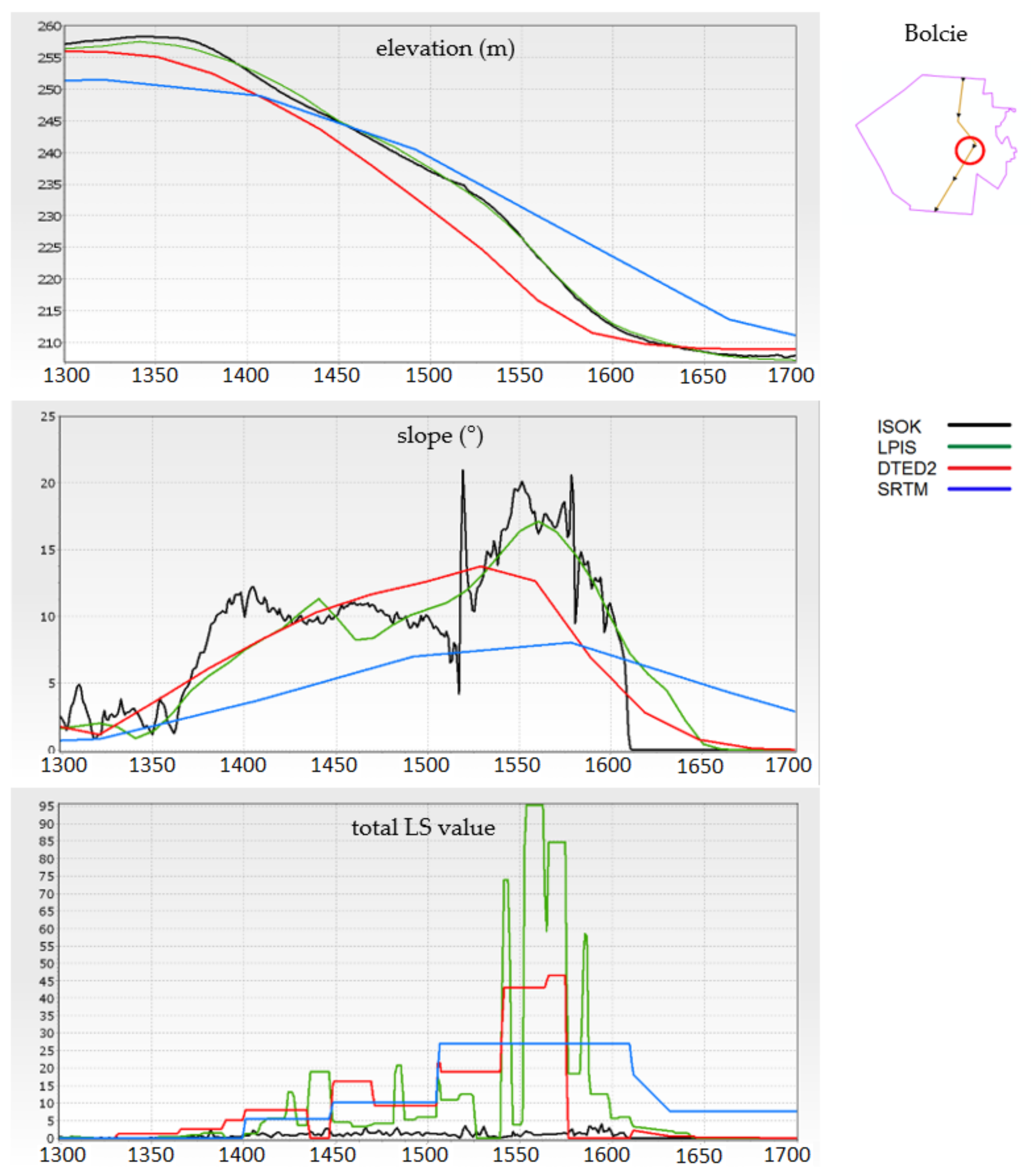
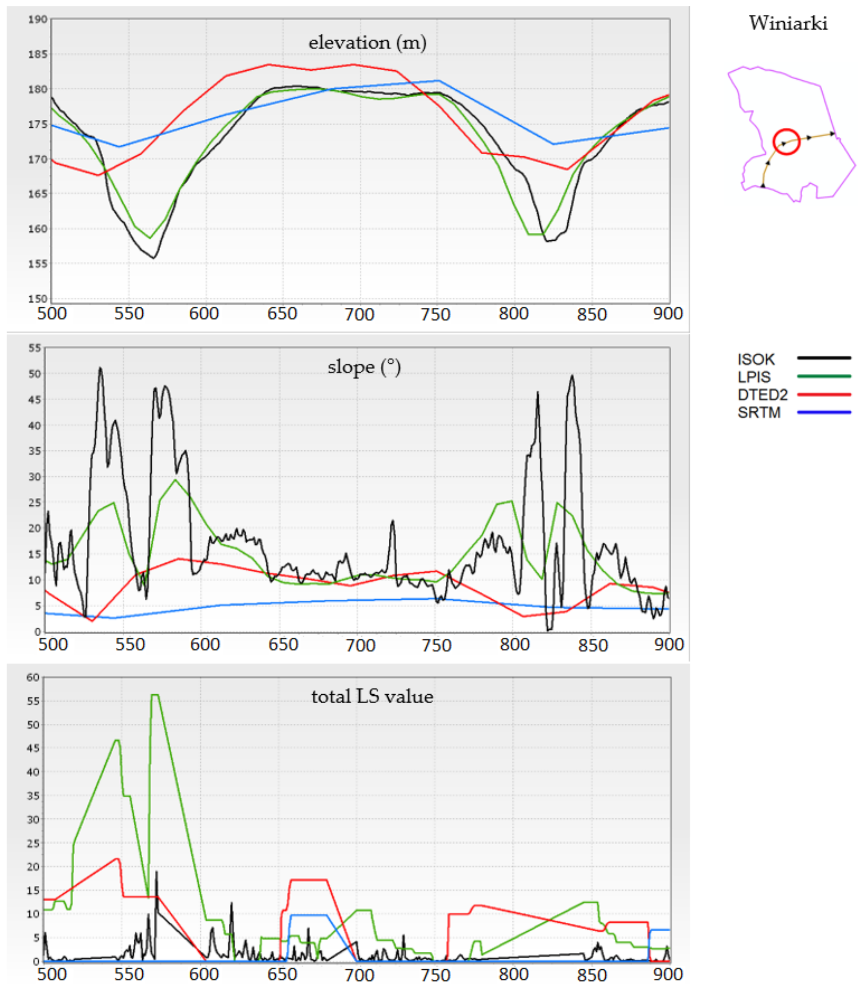
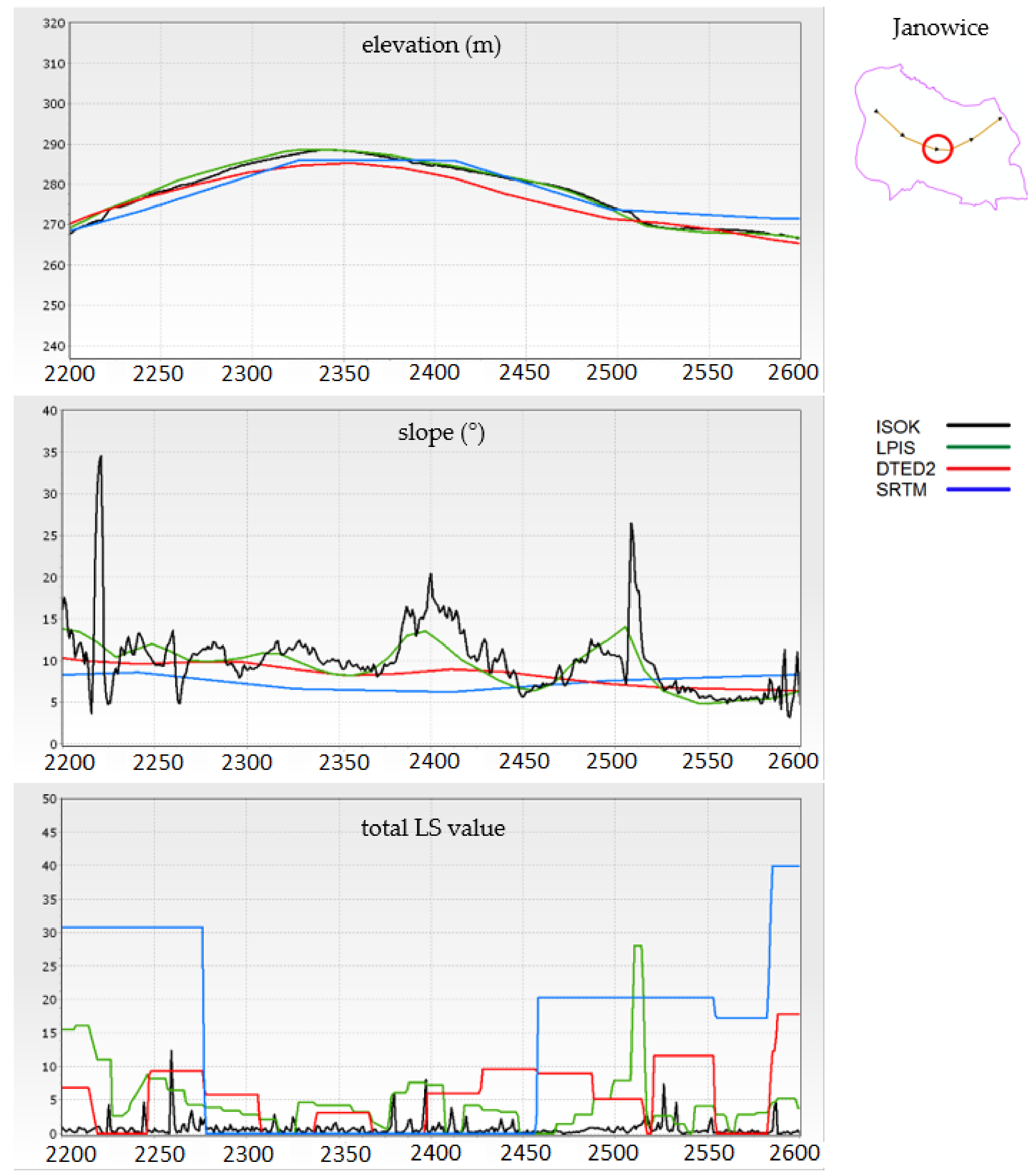
3.1. DTM Elevation and Slopes Comparison

A statistical analysis of the elevations in the individual research areas shows that there is a significant similarity of the elevation values in the analysed DTM obtained from four sources. The basic statistics of the DTM values for the research areas are presented in Table 3. Despite the significant differences in accuracy and detail, the comparative analysis of the DTM data shows that the distribution of elevation values is very similar. This is evidenced by the similarity of the histograms and by the high values of the Pearson correlation coefficients. Those values calculated for all DTM pairs are surprisingly high, with the greatest similarity in all research areas shown by the ISOK and LPIS data—the value of the correlation coefficient does not fall below 0.99. The lowest correlation was noted for the DTED2 and SRTM data, but still, the values are not lower than 0.93 (Table 4). Such high values of the Pearson coefficients are also confirmed by the analysis of the scatter plots for the DTM pairs; the closest agreement was obtained for the ISOK and LPIS data, but for all the compared DTM pairs, the points representing the pixel values of the two datasets are arranged closely along the regression line.
Despite the very high values of the correlation coefficients, the elevation differences (Δz) of LPIS, DTED2 and SRTM compared to ISOK are significant. For the less-correlated pair (ISOK and SRTM), they reached a maximum of −34.5 m (the elevation of the ISOK is smaller) and 36.3 m (the elevation of the ISOK is higher) for the agricultural areas. Even a comparison of the DTM values for the most correlated ISOK and LPIS pair shows differences on average of ±0.9 m in all research areas (Table 5).
A statistical analysis of the slope values in individual research shows that there is much less similarity in the value of this DTM derivative than in the case of the elevation values in the four analysed DTM sources. Basic statistics (Table 6) clearly shows that the maximum slope values increase with the increase of the DTM accuracy and detail (understood as the analysis of changes in the DTM derivative values for the series: SRTM → DTED → LPIS → ISOK). This is a significant change, with the maximum values increasing more than six times between SRTM and ISOK. At the same time, the average value of the slopes and the median grow—this statistical measure is subject to less fluctuations than the average, which means that, although the maximum value increases, high values of landfalls do not occur in a large part of the study area. The greater variability of slope values in the research areas is also evidenced by the increase in the value of the standard deviation along with the increase in the accuracy and detail of the analysed DTM data.
The values of the Pearson correlation coefficients of the slope values decrease in comparison to the values of the coefficients calculated for the terrain elevations (DTM values). The slopes calculated on the basis of ISOK and LPIS show the greatest similarity in all research areas—the values of the correlation coefficients do not fall below 0.75. The lowest correlation was recorded for the slopes in the ISOK and SRTM pair; the coefficient values are already lower and range from 0.36 (Bolcie study area) to 0.52 (Janowice study area) (Table 7).
An analysis of the histograms of the terrain slope values also confirms the significant variability in the distribution of the values, with an increase in the accuracy and detail of the DTM. The presence of a few pixels with relatively high slope values in each dataset was noticed (Table 8). The greater the accuracy and detail of the source data, the higher the maximum slope values.
The maximum differences in the slope values (Δs) are significant for all DTM pairs. The largest positive differences (the slope of the terrain calculated on the basis of ISOK data has a greater value) are analogically high for all the compared DTMs and range, on average, from 55° for ISOK and LPIS pair to 60° for ISOK and SRTM pair. Unexpectedly, the greatest negative differences (the slope of the area calculated on the basis of the data from ISOK has a lower value) were obtained for the ISOK and LPIS pair: −40.4° for the Janowice research area. The mean values of the absolute differences (|Δs|) do not differ significantly between the individual DTM pairs, ranging from ±2.6° for the ISOK and LPIS pair to ±4.6° for the ISOK and SRTM pair (Table 9).
When analysing the distribution of the Δs values, the greatest values are observed in the middle and lower parts of steepest slopes. Panagos [40] mentioned that the vast majority of areas in Europe have slope values of up to 50% (approx. 26.6°). This is confirmed by the results obtained for the research areas, but only if the results of the analysis using DTM data of similar accuracy and detail are compared (the analyses described in the article were carried out using EU-DEM with a spatial resolution of 25 m). The values obtained for the research areas for the DTED2 slope maps reach 29°, while, for DTM with higher accuracy and detail, the maximum values for the Janowice area (foothills) reach 46° (for LPIS DTM) and 78° (for ISOK DTM).

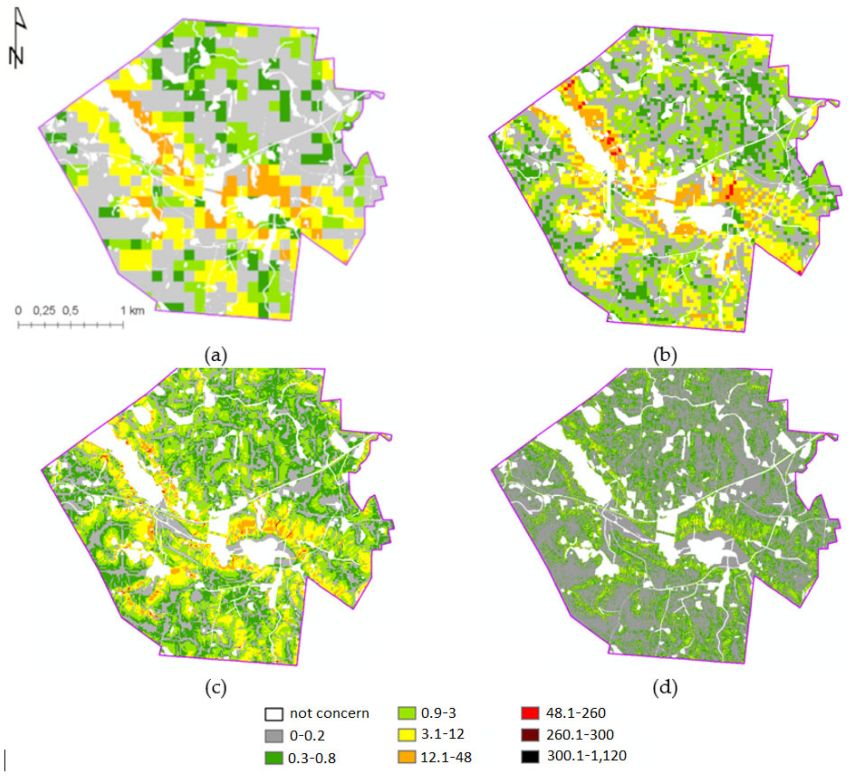
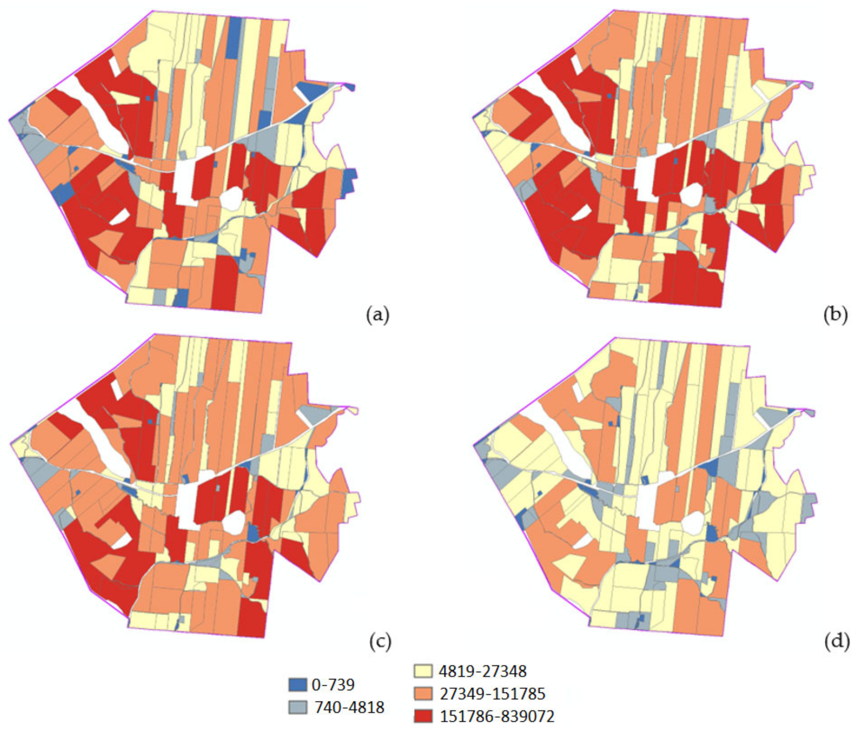
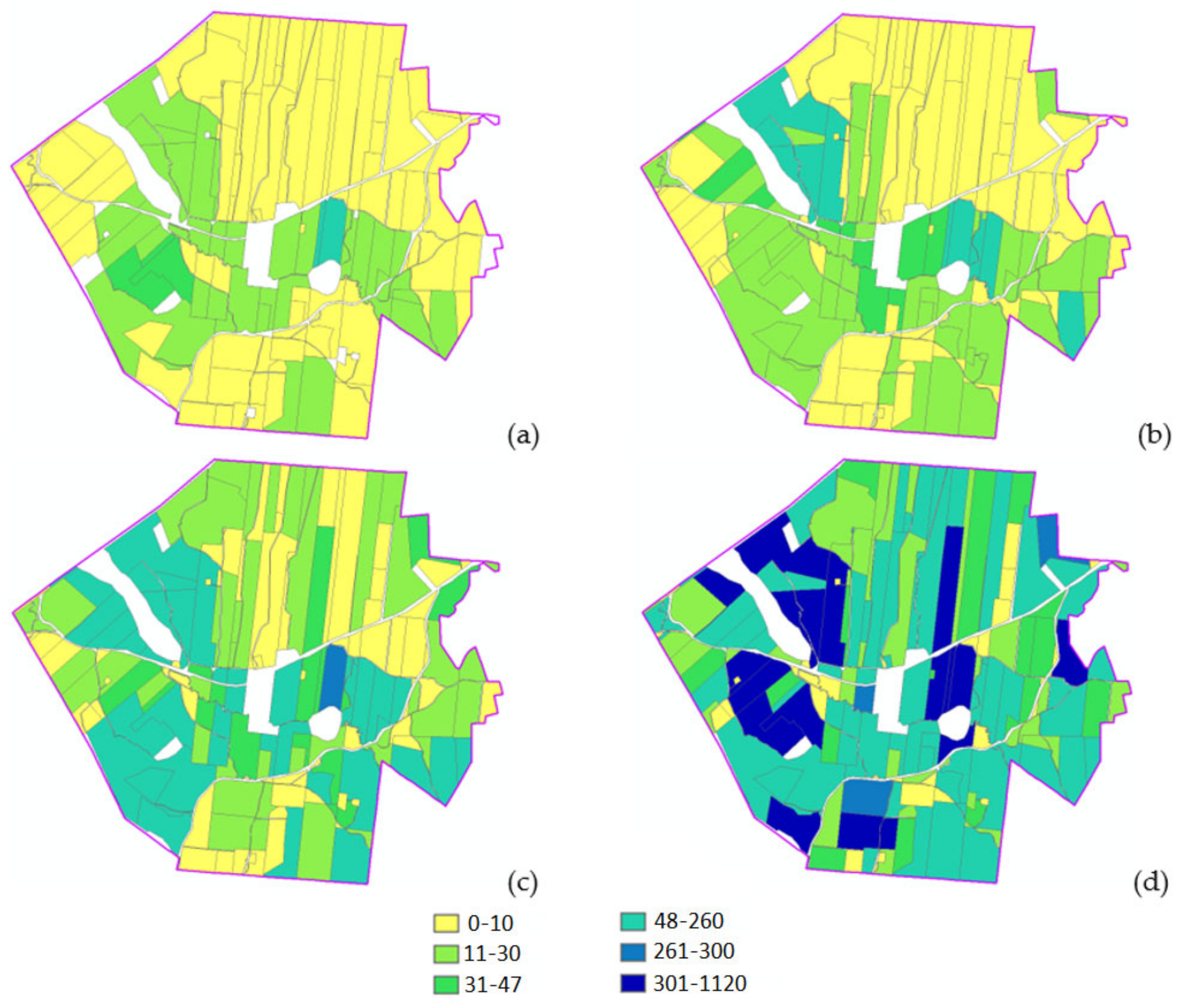
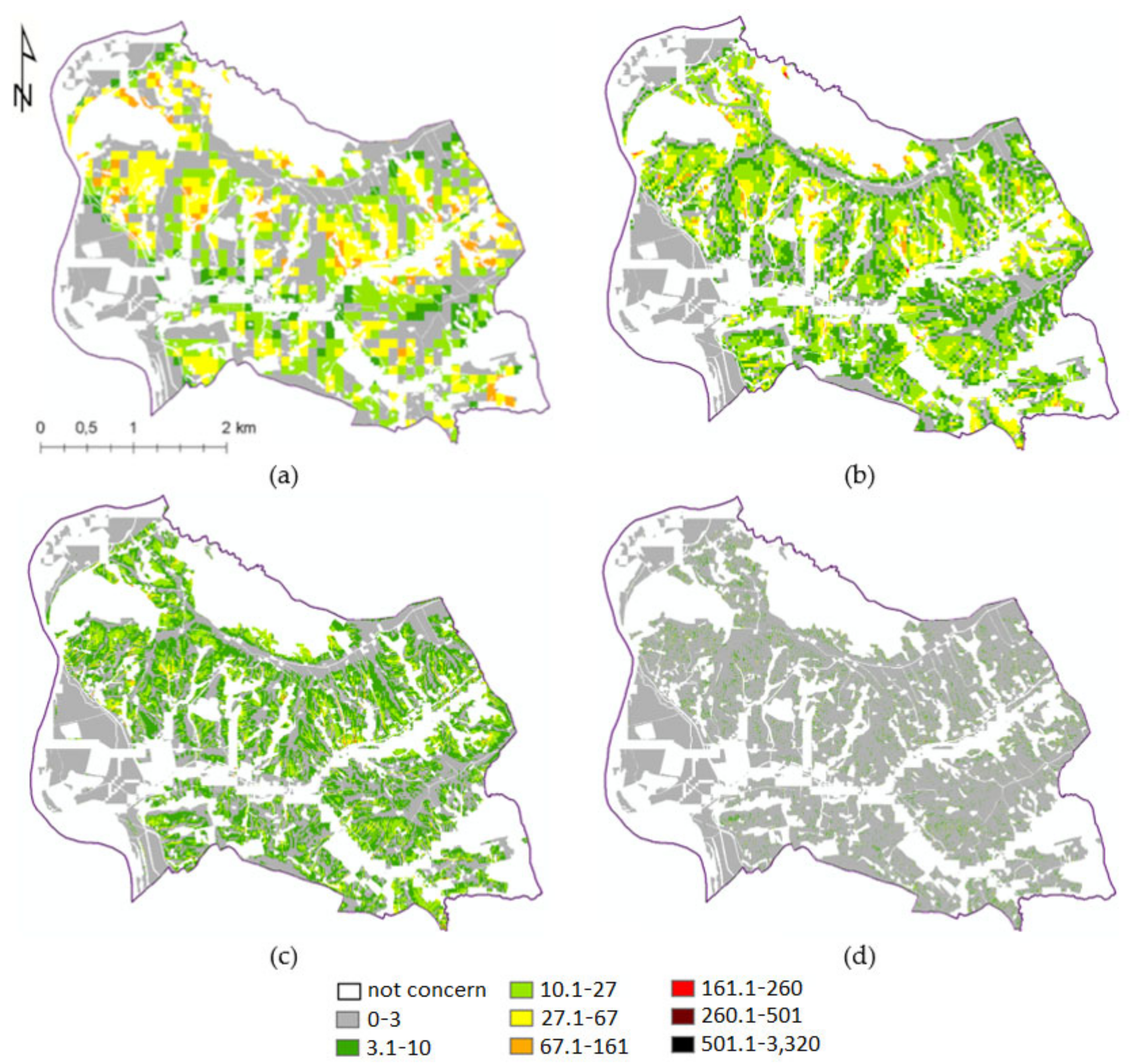
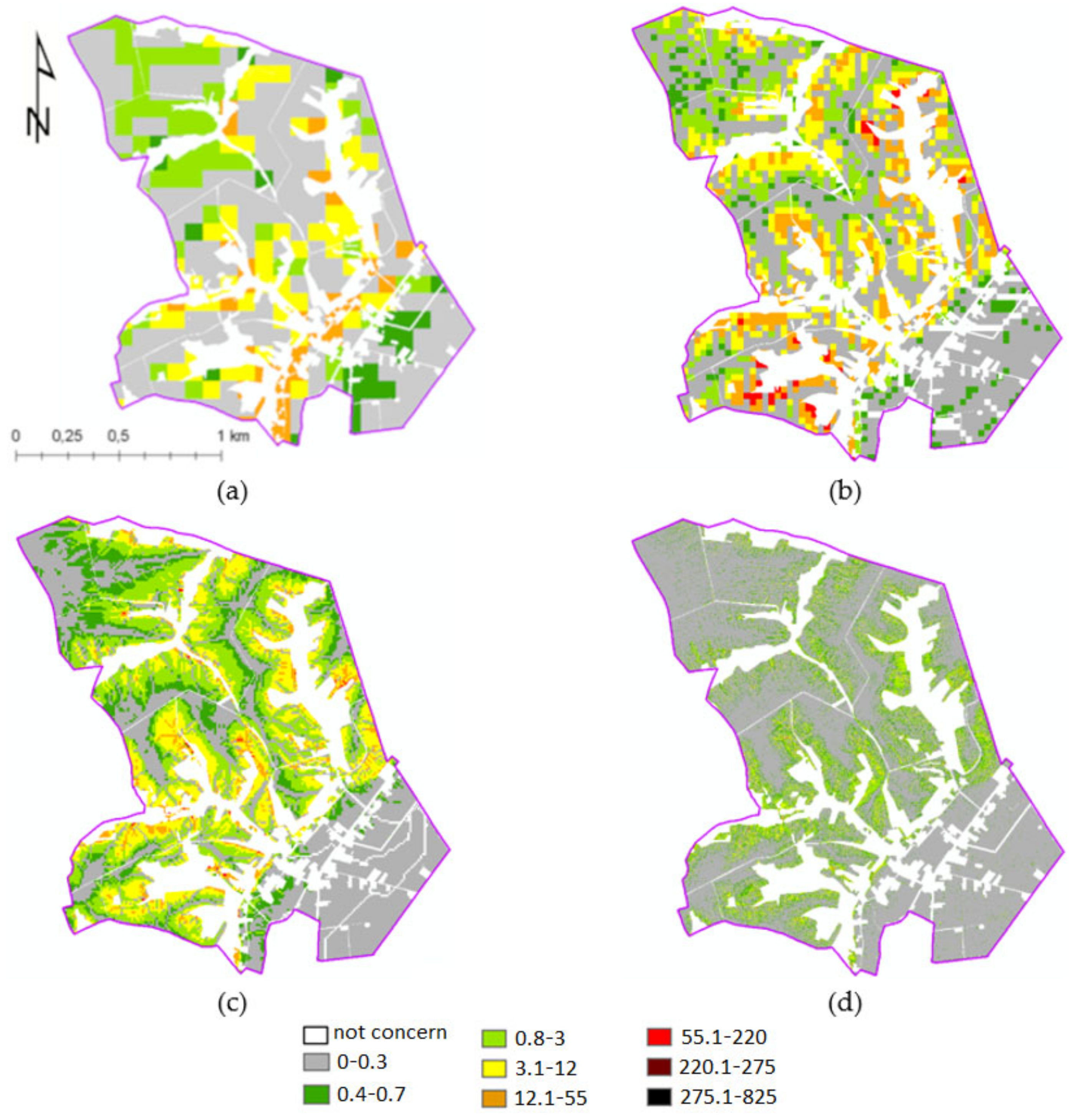
3.2. Comparison of the Total LS Factors Values

The specificity of the universal soil loss equation USLE/RUSLE results in the fact that the influence of the variability of the values of the L and S factors on the value of soil loss due to water erosion is multiplied. The total influence of the L and S factors in the soil loss equation is determined as the multiplication of their values (L * S). The first part of comparing the total LS factors values was to compare the results for each pixel (1 m × 1 m grid). The second part was to compare the statistical values after aggregating for the agricultural plots. For individual research areas, the maximum LS range was obtained up to the value of 3314.9 (for the Janowice research area) to 824.3 (for the Winiarki research area) and to 1116.8 (for the Bolcie research area); the higher values were obtained based on ISOK DTM data (Table 10).
In all the research areas, the maximum values of the total LS factor values increase consistently with the increasing accuracy and detail of the DTM source data. In the research area of Janowice, the mean and median values, as well as standard deviation, clearly decrease, along with the increase in the accuracy and detail of the source data. There is no such relationship in the Winiarki and Bolcie research areas, and the mean values and standard deviation are the highest for the LS calculated from the DTED2 data.
This is confirmed by the analysis of the terrain profiles presented in Figure 8 and in Appendix B. A comparative analysis of the elevation profiles indicates that, along with a decrease in the accuracy and detail of DTM, a process of flattening of the valleys takes place, which leads to a decrease in the length and steepness of the slope represented by the generalised source data compared to the high-resolution data. Along with the increase in the accuracy and detail of the DTM, a significant increase in the area with the total LS factor values close to 0 is noticed. This is evidenced by the total LS factor threshold values obtained for 95% and 99% of the area. The highest threshold values in the Janowice research area were observed for SRTM derivatives and, in the Winiarki and Bolcie research areas, for the DTED2 derivatives (Table 11). There is a significant discrepancy between the total LS factors threshold values for 95% and 99% of the area and the maximum of the total LS values, and this discrepancy increases with the increasing accuracy and detail of the source DTM.
The analysis of the spatial distribution and the histograms of the total LS factor values shows that the largest range of the areas with the lowest values was obtained for the results calculated on the basis of the ISOK data (Figure 9). Areas with values ranging from 0 to 1 occupy an average of 60% of the research areas for the results obtained from SRTM and 88% of the research areas for the results obtained from the ISOK data.
The analysis of the values of the Pearson correlation coefficients (Table 12) and the scatter plots indicates a significant lack of similarity of the total LS factors values obtained for the pairs of different DTM sources. Still, the lowest correlation values were obtained for the ISOK and SRTM pair—the Pearson coefficient value does not exceed 0.08 in all the research areas and indicates a complete lack of similarity of these datasets. The maximum value of the correlation coefficient was obtained for the DTED2 and SRTM pair for the Bolcie and Winiarki research areas, but it is still only a maximum of 0.44.
The distribution of the values in the profiles showing the total LS factors confirms the previously described discrepancy in the values calculated on the basis of different DTMs. In most cases, it is difficult to find the convergence of the local maximums and minimums in the graphs. There is also a noticeable, though less visible in the previously analysed statistics, overestimation of the total LS values obtained on the basis of the LPIS data—much more noticeable in the research areas of Winiarki and Bolcie. The profiles of all the compared features (elevation, slopes and the total of the LS factors values) for each of the research areas are presented in Figure 8.

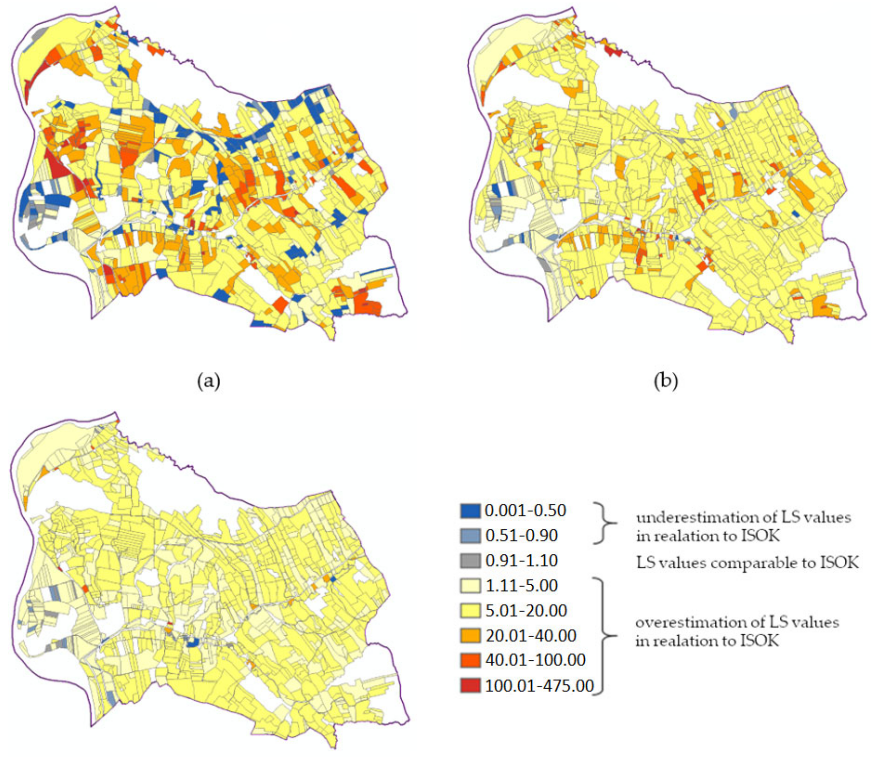
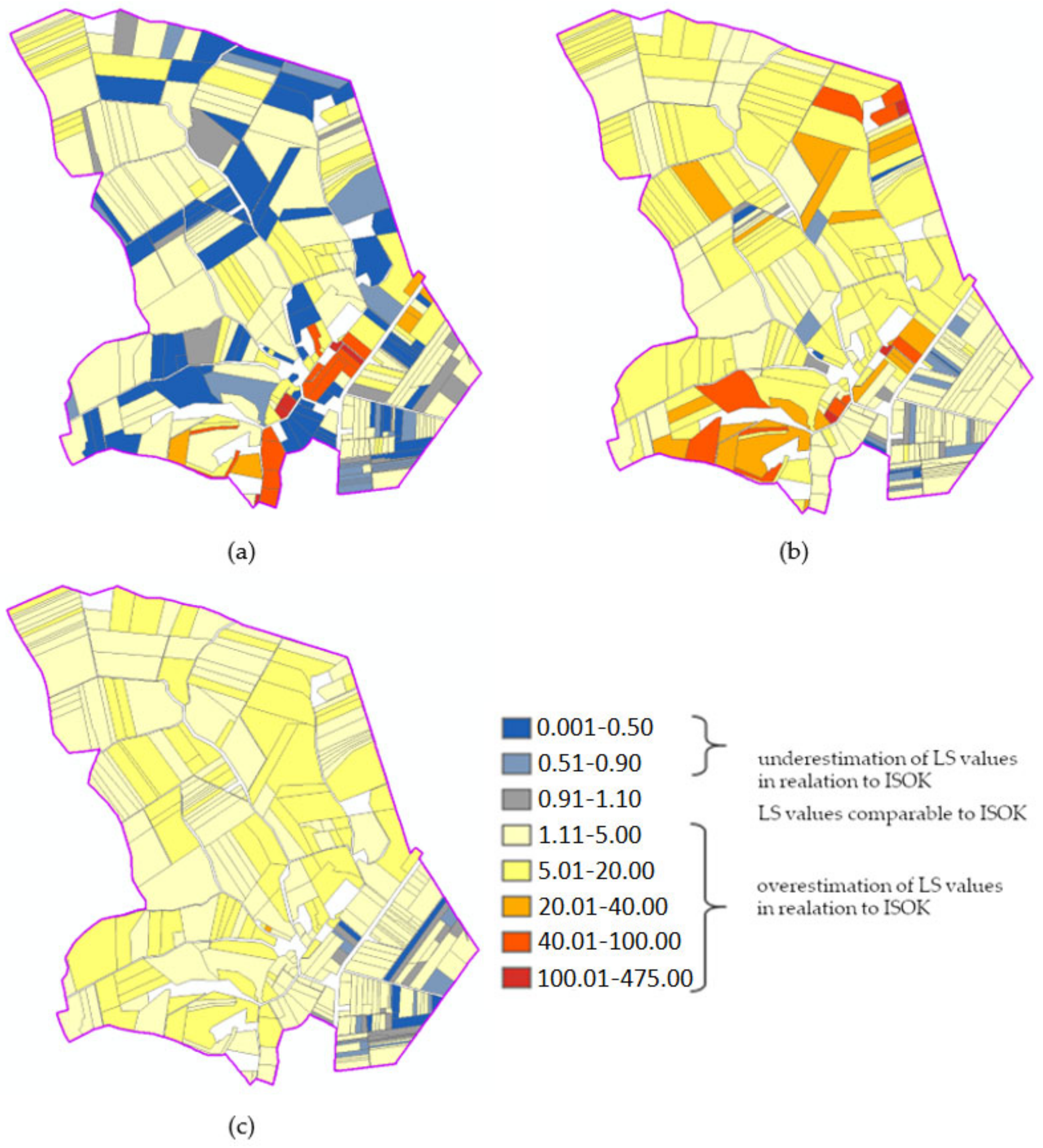
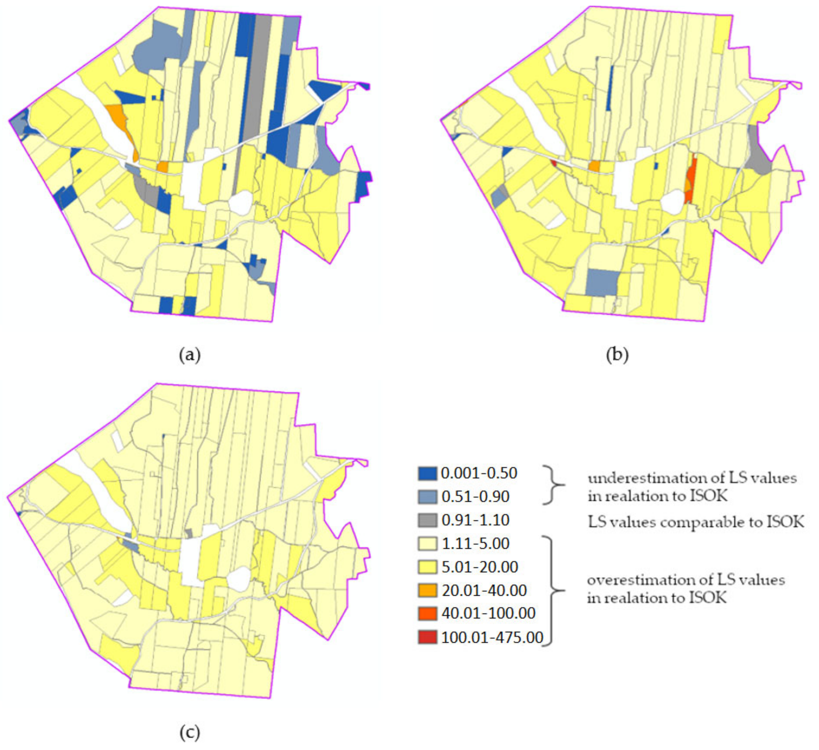
3.3. Comparison of the Total Values of the LS Factors in Agricultural Plots

The next stage was an analysis of the total LS factor values after aggregating the results in the agricultural areas (plots) designated on the basis of the data provided by ARMA. For all the agricultural plots, the LS statistical values were calculated relating to the area of the whole plot: sum, standard deviation, mean, median and maximum values. These values are presented in Table 13. Visualisation of the changes in the value of the sum of the total LS factor values in the plot and the maximum value of the total LS factor values in the plot are presented in Figure 10 and Figure 11.
Visualisations of the total LS factor values for the individual plots (Figure 10 and Figure 11) in all the research areas show:
  • a decrease in the value of the sum of the total LS factor values in the plot,
  • a decrease in the percentage of plots with high values of the sum of the total LS factor values and
  • a significant increase in the maximum of the total LS factor values in the plot as the accuracy and detail of the source DTM increases.
The obtained values of the Pearson correlation coefficients for the plots indicate a significant increase in the similarity of the total LS factor values analysed in the areas of the agricultural plots in relation to the analysis of the values at the points placed in the regular grid (1m x 1m). The highest agreement was obtained for the sum of the total LS factors values in the plot for the ISOK and LPIS pair; in all the research areas, it is a very high similarity—the values of the correlation coefficients have a value of approx. 0.96. Even for the pair of ISOK and SRTM, although the lowest, they range from 0.52 to 0.78 (Table 14).
Significantly lower values of the Pearson correlation coefficients were obtained when comparing the maximum values in the agricultural plots. These values significantly differ from each other, and the highest correlation occurs for the DTED2 and SRTM pair at the level of 0.43–0.63 and the lowest for the ISOK and SRTM pair at the level of 0.07–0.49 (Table 15).
The difference in the total LS factors values in an agricultural plot is indicated by the results of the variation index Wz, which was used to compare the LS values obtained from the SRTM, DTED2 and LPIS data with the LS values obtained from the ISOK data (Equation (2)).
As already mentioned in the description in the Methodology section, very low values of the Wz index (close to 0) indicate a significant underestimation of the total LS factor values relative to ISOK; in turn, very high Wz values indicate a significant overestimation of the total LS factors values relative to ISOK. The values of the similarity index ranging from 0.9 to 1.1 (±10%) were considered as values comparable to those obtained from ISOK. The comparison of the sums of the total LS factor values in the agriculture plots calculated on the basis of SRTM, DTED2 and LPIS against the sums of the total LS factors values calculated on the basis of ISOK for the three research areas is presented in Table 16.
The calculated values of the coefficient of variation Wz range from 0.001 (the total LS factor values with SRTM were 1000 times lower than the value obtained from ISOK) to 475 (the total LS factor values from SRTM were 475 times higher than the value obtained from ISOK). Both extreme values were obtained for the Janowice research area. The greatest differences were noticed when comparing the total LS factor values obtained from SRTM with the values obtained from ISOK. The analysis of these values revealed a significant percentage of the areas with an underestimation the total LS factors values; in all the research areas, it is a significant part of the area (Table 16). This relationship is also visible in the visualisations of the distribution of the WZ variability index (Figure 12) calculated for the total LS factors values with DTED2 and ISOK, as well as LPIS and ISOK.
The blue tones show plots with the total LS factors values underestimated in relation to ISOK; grey is comparable values and colours: yellow, orange and red are overestimated values in relation to ISOK. Plots in blue tones are scarce. The highest values of the Wz coefficient (the highest overestimation of the total LS factors values in relation to ISOK) were obtained by comparing the total LS factors values calculated with SRTM and ISOK and with DTED2 and ISOK (the Janowice and Winiarki research areas) and with DTED2 and ISOK (the Bolcie research area), which is visible in the visualisations of the Wz values distribution—the yellow, orange and red tones have the longest range. The lowest degree of underestimation and/or overestimation of the values was noted for the Wz coefficient calculated for the total LS factor values with LPIS and ISOK. The vast majority of the plots were classified in the coefficient value class with the maximum value of five (maximum five times overestimation of the total LS factor values in relation to ISOK) or the maximum value of the coefficient equal to 20 (maximum 20 times overestimation of the total LS factor values in relation to ISOK), although the share of these classes in the surface area of each area is different. The obtained values clearly show that, if a DTM with a lower accuracy and detail than ISOK is used to calculate the LS factor values, one can expect, at best, a maximum 20 times overestimation of the LS value (for DTM LPIS). Using other models with lower accuracy and detail, such as DTED2 or SRTM, one can expect an even greater overestimation and underestimation of the combined effects of both factors.

4. Discussion

Despite the advantages of the models based on the USLE/RUSLE methodology, one should also be aware of their limitations. Many authors point to the mismatch between the model and the European conditions. The empirical model was developed for the eastern part of North America, which, compared to Europe, is characterised by a different distribution and nature of precipitation, a different landscape and a different distribution of the dominant hydrological processes. Moreover, the model does not take into account gully erosion (ephemeral gullies) and crop erosion [10,40,107]. Some researchers report that comparing the modelling results with the field studies indicates that the USLE/RUSLE models usually give slightly overestimated values of soil losses or there is a noticeable overestimation of low values and an underestimation of high values [32,43,69,84]. Another important problem and challenge in erosion modelling is the assessment of the accuracy of the obtained results. It is a very difficult and complicated task, as it requires an estimation of the uncertainty of each of the equation factors, including the L and S factor values [86]. It was also noticed that the modelling results are sometimes inadequate for long slopes of complicated shapes [107]. The use of a more detailed DTM increases the length of the slopes and the complexity of their shapes. For a more complete analysis of the impact of DTM sources on the modelling results, the results obtained with the use of other, multiple-flow runoff algorithms should also be compared, as well as eroded soil deposition areas, as indicated by the works [37,60].
The research carried out indicates that the overestimation of total LS value calculated for the DTM with lower accuracy and detail concerns a much larger area of land than the underestimation that occurs in relatively small areas. However, the values of the differences obtained in this case are much higher. This is probably related to the less accurate determination of the water paths flowing down the slopes and unit upslope contributing areas using a DTM with less accuracy and detail. The obtained conclusions confirm the observations of Evans [107], who compared the results of field studies with the results of modelling using a DTM with low accuracy and detail. He showed that modelling using the USLE/RUSLE methodology results in the overestimation of values where low total LS factor values were found in the field and an underestimation of values where high total LS factor values were found in the field. Moreover, he notes that significantly high soil losses occur in small fragments of farmland. These observations are confirmed by the modelling results obtained in this study. With too-low accuracy and detail of the DTM, high values of the L and S factors are obtained, while, with a DTM with high accuracy and detail, low values of L and S are actually obtained in most of the area and very high values in small areas of the field, which indicated the areas of accumulation of runoff on slopes with significant steepness. Similar conclusions were drawn by Yang et al. [108], Fu et al. [109] and Raj et al. [110]; however, the above-mentioned studies were conducted outside Europe.
The comparison of the values of the LS factors indicates that the values obtained from the source DTMs with different accuracies and details and, resulting from them, different spatial resolutions, do not change uniformly with the increase in the DTM accuracy and detail. These dependencies cannot be described in a simple way, because for the same region, both high total LS factor values from one source DTM are obtained for the low total LS factor values from another DTM source and vice versa.
Opinions on the overestimation of the values of soil loss in the USLE/RUSLE models resulting from the literature review may be related to the inability to include natural barriers in the terrain in the available algorithms (roads, paths, fences, bushes, etc.), which are natural blockades for runoff water, often causing eroded material to be deposited. This was also mentioned by Panagos [42]. However, it seems that DTM data from airborne laser scanning (ALS) partially solves this problem.
Thus, there is a need to calibrate the existing erosion empirical models under the new conditions of access to data with high and very high accuracy and detail, as mentioned by Mitosova et al. [84].
In the literature on soil water erosion modelling, opinions can be found that the values obtained from modelling should be treated as a potential risk (qualitative approach) rather than the actual values of soil losses (quantitative approach) [12,52].
The analysis of the distribution of the obtained results of the differences in the values did not allow for a certain formulation of conclusions about which locations these differences are the greatest (e.g., the value of the slope and location in a specific part of the slope).
For the presented study, the ALS data was obtained with a scanning density of four points/m2, so generating a DTM with a resolution of 1m x 1m resulted in additional averaging of the elevation values and partially reduced the possible noise. Further data processing was not carried out on purpose, so as not to change the source data values. The next direction of research could concern ALS data filtering and comparing the results in the field studies, both the DTM values and the slope values, as well to correctly define the surface runoff paths.

5. Conclusions

As a result of the analyses carried out in accordance with the presented methodology, a significant impact of the accuracy and detail of the source elevation data on the results of calculating the values of the factors of the universal soil losses equation—slope length (L) and slope steepness (S), considered as the key of the USLE/RUSLE model factors—was demonstrated.
A different image of the terrain surface presented with the use of various DTM models (SRTM, DTED2, LPIS and ISOK), despite the high correlation of the terrain elevation values, shows a significant differentiation of the DTM derivative values. It has been proven that, when using the DTM with the lowest accuracy and detail (e.g., SRTM)—often recommended for analyses for the entire country (in accordance with the principle of “from general to detail”)—not only a significant (even a thousandfold) underestimation in one part of the studied area could be expected but, also, an overestimation in another part of the studied area of the LS factor values.
The conducted research has shown that the study of local phenomena (and soil erosion is one of them), even when carrying out an analysis over a large area, should use data of the highest accuracy and detail, because the use of data with a lower level of detail and accuracy may lead to wrong decisions. Therefore, it seems to be wrong to think that the detail of the source spatial data for an analysis should be selected adequately to the scale of the target study area, i.e., for example, in studies of the country area, data should be used at a certain level of generalisation. The modelling of local phenomena should use data adjusted to the scale of the phenomenon (and not to the scale of the study), and the visualisation of the results in smaller scales can be developed using appropriate cartographic generalisation methods.
The ALS data are characterised by high scanning density (in Poland, data from the national resource have a standard density of four or 12 points/m2). More research is needed to determine the optimal scanning density, data filtration and final raster data resolution for the proper modelling of surface water runoff phenomena.
It is necessary to pursue a responsible land use policy using the advantages of GIS technology. The identification of vulnerable areas should be performed using data of adequate accuracy and detail to prevent negative changes and protect those sites where there is a real risk of soil water erosion, and it is undoubtedly necessary. It is not possible with the use of source data that do not reflect the topography as accurately as possible. It is also important not to limit agricultural activities and not to impose special—other than those commonly used in a given area—treatments, if it is not necessary. These decisions also have financial consequences, both for agricultural producers and for the state budget.
Despite many years of research and technology development, there are still many difficulties in recognising, describing and quantifying soil water erosion, and there are still limited possibilities for predicting the intensity and frequency of erosion events [12,43,87]. In a comparative analysis of the obtained results, it may be helpful to develop a set of metadata, the provision of which would clearly indicate the source data characterisation, algorithms used and the way of their implementation. The proposed set of such metadata is included in Table 1. Moreover, another difficulty points to the up-to-date conducted research. Rainfall, land cover and topography data acquisition periods are often different, and some anti-erosion treatments may change from year to year.
Thus, some questions Boardman asked in 2006 [87]: “Where is erosion occurring? Why is it happening? How serious is it? Who does it affect? What should be the response? Can we prevent it?” are still relevant.

Funding

This research received no external funding.

Acknowledgments

The author acknowledges the Agency for Restructuring and Modernisation of Agriculture (ARiMR) for providing the plot data and the Institute of Soil Science and Plant Cultivation (IUNG) for providing the expert erosion risk estimation data used in the analysis. I would like to take this opportunity to acknowledge the time and effort devoted by the journal reviewers to improving the quality of my published work. I appreciate the detailed and useful comments that I obtained from them.

Conflicts of Interest

The author declares no conflict of interest.

Appendix A

Visualisation of the value of the total LS factors values (classes) based on SRTM (a), DTED2 (b), LPIS (c) and ISOK (d) for the Janowice and Winiarki research areas (visualisation for the Bolcie research area is in Figure 9.
Figure A1. Visualisation of the values of the total LS factor values (classes) calculated from SRTM (a), DTED2 (b), LPIS (c) and ISOK (d) for the Janowice research area.
Remotesensing 13 00678 g0a1
Figure A2. Visualisation of the total LS factor values (classes) calculated from SRTM (a), DTED2 (b), LPIS (c) and ISOK (d) for the Winiarki research area.
Remotesensing 13 00678 g0a2

Appendix B

Visualisation of the elevation (m), slopes (°) and the total LS factor values (Y-axis) calculated from all the DTM sources for a selected section of the profile (over a 400-m section) for the Janowice and Bolcie research areas (visualisation for the Winiarki research area is presented in Figure 8).
Figure A3. Visualisation of the elevation (m), slopes (°) and the total LS factor values (Y-axis) calculated from all the DTM sources for a selected section of the profile (over a 400-m section) for the Janowice research area.
Remotesensing 13 00678 g0a3
Figure A4. Visualisation of the elevation (m), slopes (°) and the total LS factor values (Y-axis) calculated from all the DTM sources for a selected section of the profile (over a 400-m section) for the Bolcie research area.
Remotesensing 13 00678 g0a4

Appendix C

Comparison of the value of the variability index Wz for the sum of the total LS factor values in the plots used for agriculture obtained from the DTM SRTM (a), DTED2 (b) and LPIS (c) against ISOK for the Janowice and Winiarki research areas (visualisation for the Bolcie research area is presented in Figure 12).
Figure A5. Comparison of the values of the variability index Wz for the sum of the total LS factor values in the plots used for agriculture obtained from the DTM SRTM (a), DTED2 (b) and LPIS (c) against ISOK for the Janowice research area.
Remotesensing 13 00678 g0a5
Figure A6. Comparison of the values of the variability index Wz for the sum of the total LS factor values in the plots used for agriculture obtained from the DTM SRTM (a), DTED2 (b) and LPIS (c) against ISOK for the Winiarki research area.
Remotesensing 13 00678 g0a6

References

  1. FAO; ITPS. Status of the World’s Soil Resources (SWSR)–Main Report; Food and agriculture organization of the United Nations and intergovernmental technical panel on soils: Rome, Italy, 2015; 650p. [Google Scholar]
  2. Montanarella, L.; Vargas, R. Global governance of soil resources as a necessary condition for sustainable development. IOP Conf. Ser. Earth Environ. Sci. 2012, 4, 559–564. [Google Scholar] [CrossRef]
  3. Eckelmann, W.; Baritz, R.; Bialousz, S.; Bielek, P.; Carré, F.; Hrušková, B.; Tóth, G. Common criteria for risk area identification according to soil threats. In Office for Official Publications of the European Communities; European Communities: Brussels, Belgium, 2006; p. 94. [Google Scholar]
  4. Renard, K.G.; Foster, G.R. Soil conservation: Principles of erosion by water. In Dryland Agriculture, Agronomy Monogr; Degne, H.E., Willis, W.O., Eds.; John Wiley & Sons, Inc.: Madison, WI, USA, 1983; Volume 23, pp. 156–176. [Google Scholar]
  5. Mitra, B.; Scott, H.D.; Dixon, J.C.; McKimmey, J.M. Applications of fuzzy logic to the prediction of soil erosion in a large watershed. Geoderma 1998, 86, 183–209. [Google Scholar] [CrossRef]
  6. Bauer, F.C.; Dyson, J.; Balsari, P.; Marucco, P. Best Management Practices to Reduce Water Pollution with Plant Protection Products from Run-Off and Erosion; European Crop Protection Association: Brussels, Brussels, 2014; Available online: http://www.topps-life.org (accessed on 21 December 2020).
  7. Janicki, G. System Stoku Zmywowego i jego Modelowanie Statystyczne–na Przykładzie Wyżyn Lubelsko-Wołyńskich (Wash Slope Systems and Their Statistical Modelling–Case Study from the Lublin-Volhynian Uplands); Wydawnictwo Uniwersytetu Marii Curie-Skłodowskiej: Lublin, Poland, 2016; p. 309. [Google Scholar]
  8. Rejman, J. Wpływ erozji wodnej i uprawowej na przekształcenie gleb i stoków lessowych. Acta Agrophysica 2006, 3, 90. [Google Scholar]
  9. Poesen, J.; Nachtergaele, J.; Verstraeten, G.; Valentin, C. Gully erosion and environmental change: Importance and research needs. Catena 2003, 50, 91–133. [Google Scholar] [CrossRef]
  10. Rejman, J.; Brodowski, R. Ocena erozji wodnej gleby lessowej na uprawach buraka cukrowego i pszenicy jarej na podstawie badań poletkowych. Procesy erozyjne na stokach użytkowanych rolniczo (metody badań, dynamika i skutki). Prace i Studia Geograficzne Uniwersytetu Warszawskiego 2010, 45, 215–228. [Google Scholar]
  11. Karydas, C.G.; Panagos, P.; Gitas, I.Z. A classification of water erosion models according to their geospatial characteristics. Int. J. Digit. Earth 2012, 7, 229–250. [Google Scholar] [CrossRef]
  12. Poesen, J. Soil erosion in the Anthropocene: Research needs. Earth Surf. Proc. Landf. 2018, 43, 64–84. [Google Scholar] [CrossRef]
  13. Rodzik, J.; Stępniewski, K. Spłukiwanie na zróżnicowanych litologicznie użytkowanych rolniczo stokach Roztocza Środkowego. In Współczesna Ewolucja rzeźby Polski, Instytut Geografii i Gospodarki Przestrzennej; Kotarba, A., Krzemień, K., Święchowicz, J., Eds.; Uniwersytet Jagielloński: Kraków, Poland, 2005; pp. 389–395. [Google Scholar]
  14. Kirkby, M. Modelling the interactions between soil surface properties and water erosion. Catena 2002, 46, 89–102. [Google Scholar] [CrossRef]
  15. Słupik, J. Rola Stoku w Kształtowaniu Odpływu w Karpatach Fliszowych; IGiPZ PAN; Zakład narodowy im. Ossolińskich: Lviv, Ukraine, 1981; p. 142. [Google Scholar]
  16. Froehlich, W.; Słupik, J. Mechanizm transportu fluwialnego i dostawy zwietrzelin do koryta w górskiej zlewni fliszowej. Przegląd Geograficzny 1986, 58, 67–87. [Google Scholar]
  17. Wischmeir, W.H.; Smith, D.D. Predicting Rainfall Erosion Losses–a Guide to Conservation Planning, Agriculture Handbook No. 537, U.S. Department of Agriculture Technical Report; U.S. Department of Agriculture: Washington, DC, USA, 1978; p. 58.
  18. Renard, K.G.; Foster, G.R.; Weesies, G.A.; McCool, D.K.; Yoder, D.C. Predicting Soil Erosion by Water: A guide to Conservation Panning with the Revised Universal Soil Loss Equation (RUSLE); United States Department of Agriculture: Washington, DC, USA, 1997; Volume 703, p. 407.
  19. Desmet, P.; Govers, G. A GIS procedure for automatically calculating the USLE LS factor on topographically complex landscape units. J. Soil Water Conserv. 1996, 51, 427–433. [Google Scholar]
  20. Zhang, L.; O’Neill, A.L.; Lacey, S. Modelling approaches to the prediction of soil erosion in catchments. Environ. Softw. 1996, 11, 123–133. [Google Scholar] [CrossRef]
  21. Rejman, J.; Usowicz, B.; Dębicki, R. Source of errors in predicting silt soil erodibility with USLE. Pol. J. Soil Sci. 1999, 32, 13–22. [Google Scholar]
  22. Schiettecatte, W.; Gabriëls, D.; Van Meirvenne, M.; Biesemans, J. Simulatie van erosiebestrijdingsmaatregelen aan de hand van het RUSLE model: Een case-studie in het stroomgebied van de Markebeek (Oost-Vlaanderen). Water Energ. Leefmilieu 1999, 18, 1–8. [Google Scholar]
  23. Liu, B.Y.; Nearing, M.A.; Shi, P.J.; Jia, Z.W. Slope length effects on soil loss for steep slopes. Soil Sci. Soc. Am. J. 2000, 64, 1759–1763. [Google Scholar] [CrossRef] [Green Version]
  24. Nyakatawa, E.Z.; Reddy, K.C.; Lemunyon, J.L. Predicting soil erosion in conservation tillage cotton production systems using the revised universal soil loss equation (RUSLE). Soil Tillage Res. 2001, 57, 213–222. [Google Scholar] [CrossRef]
  25. Rejman, J.; Usowicz, B. Evaluation of soil-loss contribution areas on loess soils in southeast Poland. Earth Surf. Proc. Land. 2002, 27, 1415–1423. [Google Scholar] [CrossRef]
  26. Grimm, M.; Jones, R.; Montanarella, L. Soil Erosion Risk in Europe, Joint Research Centre, Scientific-Technical Report EUR 19939 EN; European Commission: Brussels, Belgium, 2001; p. 38. [Google Scholar]
  27. Drzewiecki, W.; Mularz, S. Model USPED jako narzędzie prognozowania efektów erozji i depozycji materiału glebowego. Rocz. Geom. Ann. Geom. 2005, 3, 45–54. [Google Scholar]
  28. Borrelli, P.; Robinson, D.A.; Fleischer, L.R.; Lugato, E.; Ballabio, C.; Alewell, C.; Bagarello, V. An assessment of the global impact of 21st century land use change on soil erosion. Nat. Commun. 2017, 8, 1–13. [Google Scholar] [CrossRef] [Green Version]
  29. Kinnell, P.I.A. Sediment delivery from hillslopes and the Universal Soil Loss Equation: Some perceptions and misconceptions. Hydrol. Process. 2008, 22, 3168–3175. [Google Scholar] [CrossRef]
  30. Kirkby, M.; Jones, R.J.; Irvine, B.; Gobin, A.G.G.; Cerdan, O.; van Rompaey, J.J.; Grimm, M. Pan-European Soil Erosion Risk Assessment for Europe: The PESERA map, version 1 October 2003, Explanation of Special Publication Ispra 2004 No. 73 (SPI 04.73) (No. 16, 21176); Office for Official Publications of the European Communities: Brussels, Belgium, 2004; p. 21. [Google Scholar]
  31. Bagarello, V.; Ferro, V. Analysis of soil loss data from plots of differing length for the Sparacia experimental area, Sicily, Italy. Biosyst. Eng. 2010, 105, 411–422. [Google Scholar] [CrossRef]
  32. Cerdan, O.; Govers, G.; le Bissonnais, Y.; van Oost, K.; Poesen, J.; Saby, N.; Gobin, A.; Vacca, A.; Quinton, J.; Auerswald, K.; et al. Rates and spatial variations of soil erosion in Europe, A study based on erosion plot data. Geomorphology 2010, 122, 167–177. [Google Scholar] [CrossRef]
  33. Kinnell, P.I.A. Slope length factor for applying the USLE-M to erosion in grid cells. Soil Tillage Res. 2001, 58(1–2), 11–17. [Google Scholar] [CrossRef]
  34. Parveen, R.; Kumar, U. Integrated Approach of Universal Soil Loss Equation (USLE) and Geographical Information System (GIS) for Soil Loss Risk Assessment in Upper South Koel Basin, Jharkhand. J. Geogr. Syst. 2012, 4, 588–596. [Google Scholar] [CrossRef] [Green Version]
  35. Wężyk, P.; Drzewiecki, W.; Wójtowicz-Nowakowska, A.; Pierzchalski, M.; Mlost, J.; Szafrańska, B. Mapa zagrożenia erozyjnego gruntów rolnych w Małopolsce na podstawie klasyfikacji OBIA obrazów teledetekcyjnych oraz analiz przestrzennych GIS, Archives of Photogrammetry. Cartogr. Remote Sens. 2012, 24, 403–420. [Google Scholar]
  36. Zhang, H.; Yang, Q.; Li, R.; Liu, Q.; Moore, D.; He, P.; Geissen, V. Extension of a GIS procedure for calculating the RUSLE equation LS factor. Comput. Geosciences 2013, 52, 177–188. [Google Scholar] [CrossRef]
  37. Drzewiecki, W.; Ziętara, S. Wpływ algorytmu określania dróg spływu powierzchniowego na wyniki oceny zagrożenia gleb erozją wodną w skali zlewni z zastosowaniem modelu RUSLE. Rocz. Geom. Ann. Geom. 2013, 11, 57–68. [Google Scholar]
  38. Bargiel, D.; Herrmann, S.; Jadczyszyn, J. Using high-resolution radar images to determine vegetation cover for soil erosion assessments. J. Environ. Manag. 2013, 124, 82–90. [Google Scholar] [CrossRef]
  39. Oliveira, A.H.; da Silva, M.A.; Silva, M.L.N.; Curi, N.; Neto, G.K.; de Freitas, D.A.F. Development of topographic factor modeling for application in soil erosion models. In Soil Processes and Current Trends in Quality Assessment; Soriano, M.C.H., Ed.; Intech Open: London, UK, 2013; pp. 111–138. ISBN 978-953-51-1029-3. [Google Scholar] [CrossRef] [Green Version]
  40. Evelpidou, N.; Cordier, S.; Merino, A.; Figueiredo, T.D.; Centeri, C. (Eds.) Runoff Erosion, University of Athens. 2013, p. 378. Available online: http://hdl.handle.net/10198/11228 (accessed on 21 December 2020).
  41. Panagos, P.; Meusburger, K.; Ballabio, C.; Borrelli, P.; Alewell, C. Soil erodibility in Europe: A high-resolution dataset based on LUCAS. Sci. Total Environ. 2014, 479–480, 189–200. [Google Scholar] [CrossRef]
  42. Panagos, P.; Borrelli, P.; Meusburger, K. A New European Slope Length and Steepness Factor (LS-Factor) for Modeling Soil Erosion by Water. Geosciences 2015, 5, 117–126. [Google Scholar] [CrossRef] [Green Version]
  43. Panagos, P.; Borrelli, P.; Poesen, J.; Ballabio, C.; Lugato, E.; Meusburger, K.; Montanarella, L.; Alewell, C. The new assessment of soil loss by water erosion in Europe. Environ. Sci. Policy. 2015, 54, 438–447. [Google Scholar] [CrossRef]
  44. Bosco, C.; de Rigo, D.; Dewitte, O.; Poesen, J.; Panagos, P. Modelling soil erosion at European scale: Towards harmonization and reproducibility. Nat. Hazards Earth Syst. Sci. 2015, 15, 225–245. [Google Scholar] [CrossRef] [Green Version]
  45. Bagio, B.; Bertol, I.; Wolschick, N.H.; Schneiders, D.; dos Santos, M.A.N. Water erosion in different slope lengths on bare soil. Revista Brasileira de Ciência do Solo 2017, 41. [Google Scholar] [CrossRef] [Green Version]
  46. Hajigholizadeh, M.; Melesse, A.M.; Fuentes, H.R. Erosion and sediment transport modelling in shallow waters: A review on approaches, models and applications. Int. J. Environ. Res. Public Health 2018, 15, 518. [Google Scholar] [CrossRef] [Green Version]
  47. Karydas, C.G.; Panagos, P. The G2 erosion model: An algorithm for month-time step assessments. Environ. Res. 2018, 161, 256–267. [Google Scholar] [CrossRef]
  48. Schmidt, S.; Tresch, S.; Meusburger, K. Modification of the RUSLE slope length and steepness factor (LS-factor) based on rainfall experiments at steep alpine grasslands. MethodsX 2019, 6, 219–229. [Google Scholar] [CrossRef]
  49. Zachar, D. Soil Erosion; Elsevier Scientific Publishing Company: Bratislava, Slovakia, 1982; Volume 10, p. 549. [Google Scholar]
  50. Risse, L.M.; Nearing, M.A.; Nicks, A.D.; Laflen, J.M. Assessment of error in the universal soil loss equation. Soil Sci. Soc. Am. J. 1993, 57, 825–833. [Google Scholar] [CrossRef]
  51. Roose, E. Land Husbandry–Components and Strategy; FAO: Rome, Italy, 1996; Volume 70, Available online: http://www.fao.org/3/t1765e/t1765e00.htm (accessed on 21 December 2020).
  52. Tetzlaff, B.; Friedrich, K.; Vorderbrügge, T.; Vereecken, H.; Wendland, F. Distributed modelling of mean annual soil erosion and sediment delivery rates to surface waters. Catena 2013, 102, 13–20. [Google Scholar] [CrossRef]
  53. Moore, I.D.; Burch, G.J. Physical basis of the length-slope factor in the Universal Soil Loss Equation. Soil Sci. Soc. Am. J. 1986, 50, 1294–1298. [Google Scholar] [CrossRef]
  54. Moore, I.D.; Wilson, J.P. Length-slope factors for the revised universal soil loss equation: Simplified method or estimation. J. Soil Wat. Conserv. 1992, 45, 423–428. [Google Scholar]
  55. Mitasova, H.; Hofierka, J.; Zlocha, M.; Iverson, R.L. Modeling topographic potential for erosion and deposition using GIS. Int. J. Geogr. Inf. Syst. 1996, 10, 629–641. [Google Scholar] [CrossRef]
  56. Wilson, J.P.; Mitasova, H.; Wright, D.J. Water resource applications of geographic information systems. Urisa J. 2000, 12, 61–79. [Google Scholar]
  57. Liu, K.; Tang, G.; Jiang, L.; Zhu, A.X.; Yang, J.Y.; Song, X.D. Regional-scale calculation of the LS factor using parallel processing. Comput. Geosci. 2015, 78, 110–122. [Google Scholar] [CrossRef]
  58. Wilson, J.P.; Gallant, J.C. Terrain Analysis: Principles and Applications; John Wiley & Sons: New York, NY, USA, 2000; p. 479. [Google Scholar]
  59. Zhou, Q.; Lees, B.; Tang, G.A. (Eds.) Advances in Digital Terrain Analysis; Springer: Berlin, Germany, 2008; p. 462. [Google Scholar]
  60. Erskine, R.H.; Green, T.R.; Ramirez, J.A.; MacDonald, L.H. Comparison of grid-based algorithms for computing upslope contributing area. Water Resour. Res. 2006, 42, W09416. [Google Scholar] [CrossRef] [Green Version]
  61. Wilson, J.P.; Lam, C.S.; Deng, Y. Comparison of the performance of flow routing algorithms used in GIS-based hydrologic analysis. Hydrol. Process. 2007, 21, 1026–1044. [Google Scholar] [CrossRef]
  62. Xiong, L.; Tang, G.; Yan, S.; Zhu, S.; Sun, Y. Landform-oriented flow-routing algorithm for the dual-structure loess terrain based on digital elevation models. Hydrol. Process. 2013, 28, 1756–1766. [Google Scholar] [CrossRef]
  63. Renard, K.G.; Foster, G.R.; Weesies, G.A.; Porter, J.P. RUSLE: Revised universal soil loss equation. J. Soil Water Conserv. 1991, 46, 30–33. [Google Scholar]
  64. Pimentel, D.; Harvey, C.; Resosudarmo, P.; Sinclair, K.; Kurz, D.; McNair, M.; Crist, S.; Shpritz, L.; Fitton, L.; Saffouri, R.; et al. Environmental and economic costs of soil erosion and conservation benefits. Science 1995, 267, 1117–1123. [Google Scholar] [CrossRef] [PubMed] [Green Version]
  65. Józefaciuk, A.; Józefaciuk, C. Erozja Agroekosystemów, Państwowa Inspekcja Ochrony Środowiska; Biblioteka Monitoringu Środowiska: Warszawa, Poland, 1995; p. 168. [Google Scholar]
  66. Maetens, W.; Vanmaercke, M.; Poesen, J.; Jankauskas, B.; Jankauskiene, G.; Ionita, I. Effects of land use on annual runoff and soil loss in Europe and the Mediterranean: A meta-analysis of plot data. Prog. Phys. Geogr. 2012, 36, 599–653. [Google Scholar] [CrossRef]
  67. Biesemans, J.; Van Meirvenne, M.; Gabriels, D. Extending the RUSLE with the Monte Carlo error propagation technique to predict long-term average off-site sediment accumulation. J. Soil Water Conserv. 2000, 55, 35–42. [Google Scholar]
  68. Yang, D.; Kanae, S.; Oki, T.; Koike, T.; Musiake, K. Global potential soil erosion with reference to land use and climate changes. Hydrol. Process. 2003, 17, 2913–2928. [Google Scholar] [CrossRef]
  69. Hohwieler, N.K. Quantification of soil erosion in the Alps: Measurement and Modeling. Ph.D. Thesis, University of Basel, Basel, Switzerland, 2010; p. 101. [Google Scholar]
  70. Drzewiecki, W.; Wężyk, P.; Pierzchalski, M.; Szafrańska, B. Quantitative and qualitative assessment of soil erosion risk in Małopolska (Poland), supported by an object-based analysis of high-resolution satellite images. Pure Appl. Geophys. 2014, 171, 867–895. [Google Scholar] [CrossRef] [Green Version]
  71. Kowalczyk, A.; Twardy, S. Wielkość erozji wodnej obliczona metodą USLE. Woda-Środowisko-Obszary Wiejskie 2012, 12, 83–92. Available online: https://portal.issn.org/resource/ISSN/1642-8145 (accessed on 21 December 2020).
  72. Ferreira, V.; Panagopoulos, T. Predicting Soil Erosion Risk at the Alqueva Dam Watershed (No. 2012-4); CIEO-Research Centre for Spatial and Organizational Dynamics, University of Algarve: Faro, Portugal, 2012. [Google Scholar]
  73. Ferreira, V.; Panagopoulos, T. Seasonality of soil erosion under Mediterranean conditions at the Alqueva dam watershed. Environ. Manag. 2014, 54, 67–83. [Google Scholar] [CrossRef]
  74. Csáfordi, P.; Pődör, A.; Bug, J.; Gribovsyki, Z. Soil erosion analysis in a small forested catchment supported by ArcGIS Model Builder. Acta Silvatica et Lignaria Hungarica 2012, 8, 39–56. [Google Scholar] [CrossRef] [Green Version]
  75. Conforti, M.; Buttafuoco, G.; Rago, V.; Aucelli, P.P.; Robustelli, G.; Scarciglia, F. Soil loss assessment in the Turbolo catchment (Calabria, Italy). J. Maps. 2016, 12, 815–825. [Google Scholar] [CrossRef]
  76. Capolongo, D.; Pennetta, L.; Piccarreta, M.; Fallacara, G.; Boenzi, F. Spatial and temporal variations in soil erosion and deposition due to land-levelling in a semi-arid area of Basilicata (Southern Italy). Earth Surf. Process. Landf. 2008, 33, 364–379. [Google Scholar] [CrossRef]
  77. Pregnolato, M.; D’Amico, M. Water Regime in the Alpine Space: Soil Erosion in a Changing Environment. Tech. Rep. 2011, 84. [Google Scholar]
  78. Ducci, D.; Giugni, M.; Zampoli, M. Evaluation of soil erosion process of the Tusciano river basin. In Proceedings of the COST Soil and Hillslope Management using Analysis and Runoff-Erosion Models: A Critical Evaluation of Current Technique, Florence, Italy, 7–9 May 2007; CNR-IRPI National Research Council Research Institute for GeoHydrological Protection: Bari, Italy, 2007; pp. 30–36. [Google Scholar]
  79. Rodriguez, J.L.G.; Suarez, M.C.G. Methodology for estimating the topographic factor LS of RUSLE3D and USPED using GIS. Geomorphology 2012, 175, 98–106. [Google Scholar] [CrossRef]
  80. Barrena-González, J.; Rodrigo-Comino, J.; Gyasi-Agyei, Y.; Pulido, M.C. Applying the RUSLE and ISUM in the Tierra de Barros Vineyards (Extremadura, Spain) to Estimate Soil Mobilisation Rates. Land 2020, 9, 93. [Google Scholar] [CrossRef] [Green Version]
  81. Covelli, C.; Cimorelli, L.; Pagliuca, D.N.; Molino, B.; Pianese, D. Assessment of Erosion in River Basins: A Distributed Model to Estimate the Sediment Production over Watersheds by a 3-Dimensional LS Factor in RUSLE Model. Hydrology 2020, 7, 13. [Google Scholar] [CrossRef] [Green Version]
  82. Xanthakis, M.; Minetos, P.; Lisitsa, G.; Kamari, G. Numerical Modelling of Soil Erosion on Cephalonia Island, Greece Using Geographical Information Systems and the Revised Universal Soil Loss Equation (RUSLE). Proceedings 2018, 2, 618. [Google Scholar] [CrossRef] [Green Version]
  83. Zhao, Z.; Benoy, G.; Chow, T.; Rees, H.; Daigle, J.-L.; Meng, F.-R. Impacts of Accuracy and Resolution of Conventional and LiDAR Based DEMs on Parameters Used in Hydrologic Modeling. Water Resour. Manag. 2010, 24, 1363–1380. [Google Scholar] [CrossRef]
  84. Mitasova, H.; Barton, C.M.; Ullah, I.I.T.; Hofierka, J.; Harmon, R.S. GIS-based soil erosion modeling. In Treatise in Geomorphology: Vol. 3 Remote Sensing and GI Science in Geomorphology; Shroder, J., Bishop, M., Eds.; Academic Press: San Diego, CA, USA, 2013; pp. 228–258. [Google Scholar] [CrossRef]
  85. Holata, L.; Kapička, J.; Světlík, R.; Žížala, D. Risk Management as a Stimulus for a Settlement and Landscape Transformation? Soil Erosion Threat Assessment in the Fields of Four Deserted Villages Based on LiDAR-Derived DEMs and ‘USLE’. In Proceedings of the GIS Ostrava, Ostrava, Czech Republic, 22–24 March 2017; Springer: Berlin, Germany, 2017; pp. 131–147. [Google Scholar]
  86. Harmon, R.S.; Doe, W.W., III (Eds.) Landscape Erosion and Evolution Modeling; Springer: Berlin, Germany, 2001; p. 540. [Google Scholar]
  87. Boardman, J. Soil erosion science: Reflections on the limitations of current approaches. Catena 2006, 68, 73–86. [Google Scholar] [CrossRef]
  88. Lee, G.S.; Lee, K.H. Scaling effect for estimating soil loss in the RUSLE model using remotely sensed geospatial data in Korea. Hydrol. Earth Syst. Sci. Discuss. 2006, 3, 135–157. Available online: https://hal.archives-ouvertes.fr/hal-00298647 (accessed on 21 December 2020).
  89. Zhu, Q.; Yang, X.; Yu, Q. Assess the topographic resolution impact on soil loss. In Proceedings of the 2016 IEEE International Geoscience and Remote Sensing Symposium (IGARSS), Beijing, China, 10–15 July 2016; pp. 6055–6058. [Google Scholar] [CrossRef]
  90. Thomas, I.A.; Jordan, P.; Shine, O.; Fenton, O.; Mellander, P.E.; Dunlop, P.; Murphy, P.N.C. Defining optimal DEM resolutions and point densities for modelling hydrologically sensitive areas in agricultural catchments dominated by microtopography. Int. J. Appl. Earth Obs. Geoinf. 2017, 54, 38–52. [Google Scholar] [CrossRef] [Green Version]
  91. Hrabalíková, M.; Janeček, M. Comparison of different approaches to LS factor calculations based on a measured soil loss under simulated rainfall. Soil Water Res. 2017, 12, 69–77. [Google Scholar] [CrossRef] [Green Version]
  92. Drzewiecki, W.; Mularz, S.; Twardy, S.; Kopacz, M. Próba kalibracji modelu RUSLE/SDR dla oceny ładunku zawiesiny wprowadzanego do Zbiornika Dobczyckiego ze zlewni bezpośredniej. Archiwum Fotogrametrii, Kartografii i Teledetekcji 2008, 18, 83–98. [Google Scholar]
  93. Panagos, P.; Meusburger, K.; van Liedekerke, M.; Alewell, C.; Hiederer, R.; Montanarella, L. Assessing soil erosion in Europe based on data collected through a European Network. Soil Sci. Plant Nutr. 2014, 60, 15–29. [Google Scholar] [CrossRef] [Green Version]
  94. Van der Knijff, J.M.; Jones, R.J.A.; Montanarella, L. Soil Erosion Risk Assessment in Europe. Scientific-Technical Reports, European Soil Bureau, Joint Research Centre; EUR 19044 EN; European Commission: Brussels, Belgium, 2000; p. 34. [Google Scholar]
  95. Molnar, D.; Julien, P. Estimation of upland erosion using GIS. Comput. Geosci. 1998, 24, 183–192. [Google Scholar] [CrossRef]
  96. Liu, H.H.; Fohrer, N.; Hormann, G.; Kiesel, J. Suitability of S factor algorithms for soil loss estimation at gently sloped landscapes. Catena 2009, 77, 248–255. [Google Scholar] [CrossRef]
  97. Wessel, B. TanDEM-X Ground Segment–DEM Products Specification Document, Public Document TD-GS-PS-0021, (3.0); Public Document TD-GS-PS-0021; DLR: Oberpfaffenhofen, Germany, 2018; Issue 3.2, p. 49. [Google Scholar]
  98. Rizzoli, P.; Martone, M.; Gonzalez, C.; Wecklich, C.; Tridon, D.B.; Bräutigam, B.; Bachmann, M.; Schulze, D.; Fritz, T.; Huber, M.; et al. Generation and performance assessment of the global TanDEM-X digital elevation model. ISPRS J. Photogramm. Remote Sens. 2017, 132, 119–139. [Google Scholar] [CrossRef] [Green Version]
  99. Bac-Bronowicz, J.; Berus, T.; Karyś, A.; Kowalski, P.; Olszewski, R. Koncepcja i realizacja intemetowego serwisu geoinformacyjnego udostępniającego dane referencyjne i tematyczne. Rocz. Geom. Ann. Geom. 2008, 6, 15–22. [Google Scholar]
  100. Kurczyński, Z. Fotogrametria; Wydawnictwo Naukowe PWN SA: Warszawa, Poland, 2015; p. 695. [Google Scholar]
  101. Woźniak, P. Wykorzystanie Danych Przestrzennych do Opracowania Map Zagrożenia Powodziowego i Map Ryzyka Powodziowego, Materiały Konferencyjne “Informatyczny System Osłony Kraju Przed nadzwyczajnymi Zagrożeniami. Opracowanie i Wykorzystanie Map Zagrożenia Powodziowego i Map Ryzyka Powodziowego”; GUGiK: Warszawa, Poland, 2014. [Google Scholar]
  102. Floras, S.A.; Sgouras, I.D. Use of geoinformation techniques in identifying and mapping areas of erosion in a hilly landscape of central Greece. Int. J. Appl. Earth Obs. Geoinf. 1999, 1, 68–77. [Google Scholar] [CrossRef]
  103. Pennock, D.J. Terrain attributes, landform segmentation, and soil redistribution. Soil Tillage Res. 2003, 69, 15–26. [Google Scholar] [CrossRef]
  104. Leighton-Boyce, G.; Doerr, S.H.; Shakesby, R.A.; Walsh, R.P.D. Quantifying the impact of soil water repellency on overland flow generation and erosion: A new approach using rainfall simulation and wetting agent on in situ soil. Hydrol. Process. 2007, 21, 2337–2345. [Google Scholar] [CrossRef]
  105. Karaburun, A. Estimation of C factor for soil erosion modeling using NDVI in Buyukcekmece watershed. Ozean J. Appl. Soc. 2010, 3, 77–85. [Google Scholar]
  106. Tarboton, D.G. A new method for the determination of flow directions and upslope areas in grid digital elevation models. Water Resour. Res. 1997, 33, 309–319. [Google Scholar] [CrossRef] [Green Version]
  107. Evans, R. An alternative way to assess water erosion of cultivated land–field-based measurements: And analysis of some results. Appl. Geogr. 2002, 22, 187–207. [Google Scholar] [CrossRef]
  108. Yang, D.; Herath, S.; Musiake, K. Spatial resolution sensitivity of catchment geomorphologic properties and the effect on hydrological simulation. Hydrol. Process. 2001, 15, 2085–2099. [Google Scholar] [CrossRef]
  109. Fu, S.; Cao, L.; Liu, B.; Wu, Z.; Savabi, M.R. Effects of DEM grid size on predicting soil loss from small watersheds in China. Environ. Earth Sci. 2015, 73, 2141–2151. [Google Scholar] [CrossRef]
  110. Raj, A.R.; George, J.; Raghavendra, S.; Kumar, S.; Agrawal, S. Effect of DEM resolution on LS factor computation. ISPRS Int. Arch. Photogramm. Remote Sens. Spat. Inf. Sci 2018, XLII-5, 315–321. [Google Scholar] [CrossRef] [Green Version]
Figure 1. The research areas localisation: 1—Janowice, 2—Winiarki and 3—Bolcie (hypsometric map from WMS: http://mapy.geoportal.gov.pl; (accessed on 21 December 2020); Ref. Syst: EPSG 2180).
Remotesensing 13 00678 g001
Figure 2. Janowice research area: slope map with hill shade effects (data source: ALSdigital terrain model (DTM) processing—1 m × 1 m spatial resolution) (a) and water erosion risk based on The Institute of Soil Science and Plant Cultivation (IUNG) expert classification from level 0—no risk to level 5—very high risk and 40 m × 40 m spatial resolution (b).
Remotesensing 13 00678 g002
Figure 3. Winiarki research area: slope map with hill shade effects (data source: ALS DTM processing—1 m × 1 m spatial resolution) (a) and water erosion risk based on the IUNG expert classification from level 0—no risk to level 5—very high risk: 40 m × 40 m spatial resolution (b).
Remotesensing 13 00678 g003
Figure 4. Bolcie research area: slope map with hill shade effects (data source: ALS DTM processing—1 m × 1 m spatial resolution) (a) and water erosion risk based on the IUNG expert classification from level 0—no risk to level 5—very high risk: 40 m × 40 m spatial resolution (b).
Remotesensing 13 00678 g004
Figure 5. The methodology of a comparative analysis of the DTM and slopes values (stage 2).
Remotesensing 13 00678 g005
Figure 6. The methodology of calculating and comparing the values of the slope length (L) and steepness (S) factors (step 3).
Remotesensing 13 00678 g006
Figure 7. The methodology of the comparative analysis of the total LS factors value (stage 4).
Remotesensing 13 00678 g007
Figure 8. Visualisation of the elevation (m), slopes (°) and the total LS factor values (Y-axis) calculated from all the DTM sources for a selected section of the profile (over a 400-m section) of the Winiarki research area (additional visualisations for Janowice and Bolcie research areas are presented in Appendix B).
Remotesensing 13 00678 g008
Figure 9. Visualisation of the total LS factor values (classes) based on SRTM (a), DTED2 (b), LPIS (c) and ISOK (d) for the Bolcie research area (additional visualisations for Janowice and Winiarki research areas are presented in the Appendix A).
Remotesensing 13 00678 g009
Figure 10. Visualisation of the sum of the total LS factors values in agriculture plots based on SRTM (a), DTED2 (b), LPIS (c) and ISOK (d) of the Bolcie research area.
Remotesensing 13 00678 g010
Figure 11. Visualisation of the maximum of the total LS factor values in the agriculture plots based on SRTM (a), DTED2 (b), LPIS (c) and ISOK (d) of the Bolcie research area.
Remotesensing 13 00678 g011
Figure 12. Comparison of the values of the variability index Wz for the sum of the LS factor values in the plots used for agriculture obtained from the DTM SRTM (a), DTED2 (b) and LPIS (c) against ISOK for the Bolcie research area (additional visualisations for the Janowice and Winiarki research areas are presented in Appendix C).
Remotesensing 13 00678 g012
Table 1. Review of soil loss results from selected European studies in the period 1996–2020, and a comparison with the results of field studies from USA and Europe investigations. Equation: U (Universal Soil Loss Equation (USLE)) and R (Revised Universal Soil Loss Equation), flow: flow length (l) and unit contribution area (a) and flow algorithm: single flow direction (SFD) and multiple flow direction (MFD).
NoMax Loss t/ha/yMean Loss t/ha/yEquationDTM SourceDTM res. [m]FlowFlow AlgorithmResearch DateResearch LocalisationResearch AreaRegionCountryPublication DateBibliography
-20.5Uchart/table---60′ 70′USAfield-USA1978[17]
-28.1Rchart/table---80′Indianafield-USA1991[63]
-17field- 1955–1995 field-Europe1995[64]
-0.84field- 50′ field-Europe1995[65]
-10–20field----1950–20101056 plotsfield-Europe2012[66]
1-0.5UTopo map 10k5aMFD90′Ganspoel catchment2.1 km²FlandersBE1996[19]
2-4.1RTopo map 10k10lSFD (Rho8) 1993–1995Kemmelbeek Watershed1075 haFlandersBE2000[67]
3-11.1RUSGS HYDRO1k1,000l-80′---Europe2003[68]
4>201USRTM100l-----Europe2010[32]
5161.18USwisstopo25l-2006/2007Urseren Valley67 km²Central CH AlpsCH2010[69]
697.8-RSRTM90a---15,183 km²Małopolskie VoivodshipPL2012[35]
57>30-U-21l-2009test field near Gorajec84 km²Roztocze regionPL2013[38]
8>154.3U-20aMFD (D∞)2004–2008-21,115 km²HesseDE2013[52]
913.83.8Uaerial images15a-1981–2009-15,183 km²Małopolskie PL2014[70]
10-19U--l--part of Bystrzyca Dusznicka 8.8 km²Dolnośląskie PL2012[71]
11>20014.1RTopo map14.98a--Herdade do Roncão739 haregion of AlentejoPT2012[72]
12>3015.1RSRTM30a-2006–2009Alqueva reservoir250 km²region of AlentejoPT2014[73]
136.40.5UFÖMI. DDM-55a 2008–2009Farkas Ditch catchment0.6 km2Sopron HillsHU2012[74]
14405.65RTopo map 10k-l-2006Turbolo catchment30 km²CalabriaIT2016[75]
15>409.02R-25 & 10aMFD (D∞)1955–2002Salandrella-Cavone 74 km²Basilicata RegionIT2008[76]
16>501.8RRegione Lombardia90 & 20a--Adda river basin5170 km²Rhaetian AlpsIT. CH2011[77]
17>50-R-90a--Upper Soča/Isonzo basin1300km²Julian AlpsSLO, IT2011[77]
18>100-R-90a-1985–2005Alpine River Inn basin26,000 km²-CH, AT, DE, IT2011[77]
195458.657R-20l-2001Tusciano river basin261 km²Campania RegionIT2007[78]
20204.6-R-10aMFD (D∞) -Arroyo del Lugar basin768.62 haGuadalajaraES2012[79]
2145.817.4R-3a-2018Tierra de Barros20 haprovince of Badajoz ES2020[80]
2211,68071.4R-5aMFD-Camastra river basin350 km²Basilicata RegionIT2020[81]
23>7512.8R-20--2002 & 2012Cephalonia Island773 km²Cephalonia IslandGR2018[82]
24>502.46REU-DEM (STRM + ASTER GDEM)25aMFD (TFM)2000s---Europe2015[43]
25>500.89RASTER GDEM / SRTM250aMFD2001–2012---World2017[28]
Table 2. Summary of the commonly used elevation data for the area of Poland. DTM: digital terrain model and DSM: digital surface model.
Dataset NameModel TypeAbsolute Height AccuracySpatial Resolution (GRID Structure)Up-to-Date
SRTMDSM1.6 m–7.2 m 30 m / 90 m2000
FDEM / HDEMDSM0.8 m/4–8 m6 m2017 [97]
IDEM2 m [98]12 m2010–2015
TanDEM-X<10 m [98]90 m2010–2015
DTED2DTM<10 m
1.5 m–7.5 m
30 m1980 [99]
ASTER
GDEM 2
DSM7 m–14 m 30 m2011
ALOS World 3D v.2.2DSM5 m30 m2015–2018
EUDEMDSM7 m25 m2011
LPISDTM0.6 m–0.9 m
0.9 m–1.5 m
10 m
15 m
2010–2018
ALS / ISOKDTM. DSM
DTM. DSM
0.10 m (st. I)
0.25 m (st. II) [100]
0.5 m
1 m
2010–2018
2010–2018
Table 3. Summary of the basic statistics characterising the elevations for all the DTM sources in the 3 research areas.
Data SourceMinMaxMeanMedianStandard DeviationRange Min-Max
Janowice
SRTM198410285.528854.7212
DTED2202416287.128953.8214
LPIS200.2418.1287.5289.654.3218
ISOK201.0418.0287.4289.454.3217
Winiarki
SRTM135199175.418318.764
DTED2139206178.318418.967
LPIS139.1204.6178.8186.219.766
ISOK138.6205.2179.4186.819.767
Bolcie
SRTM204260238.824111.956
DTED2207264241.324412.857
LPIS205.4264.4241.0243.612.759
ISOK206.0266.5241.7244.512.761
Table 4. Comparison of the DTM Pearson correlation coefficient values for all DTM sources in the 3 research areas.
Janowice
ISOKLPISDTED2SRTM
ISOK1.0001.0000.9980.991
LPIS 1.0000.9980.992
DTED2 1.0000.989
SRTM 1.000
Winiarki
ISOKLPISDTED2SRTM
ISOK1.0000.9980.9720.967
LPIS 1.0000.9750.969
DTED2 1.0000.956
SRTM 1.000
Bolcie
ISOKLPISDTED2SRTM
ISOK1.0000.9980.9780.942
LPIS 1.0000.9790.949
DTED2 1.0000.933
SRTM 1.000
Table 5. Comparison of the differences in the elevation values from DTM of lower accuracy and detail (SRTM, DTED2 and LPIS) to ISOK (minimum, maximum and mean of the absolute value ǀΔzǀ of the differences).
ISOK-SRTM (m)ISOK-DTED2 (m)ISOK-LPIS (m)
Research Areamin
Δz
max
Δz
mean
ǀΔzǀ
min
Δz
max
Δz
mean
ǀΔzǀ
min
Δz
max
Δz
mean
ǀΔzǀ
Janowice−34.536.3± 5.8−27.322.1± 2.5−11.014.0± 0.7
Winiarki−24.434.5± 5.4−23.435.3± 3.0−14.012.7± 1.0
Bolcie−22.425.1± 4.1−13.120.5± 2.0−6.07.9± 0.9
Table 6. Summary of the basic statistics of the slope values (°) in the 3 research areas.
Data SourceMinMaxMeanMedianStandard DeviationRange Min-Max
Janowice
SRTM0.016.46.57.13.316.4
DTED20.027.47.98.24.327.4
LPIS0.041.58.68.75.141.5
ISOK0.065.99.48.86.565.9
Winiarki
SRTM0.012.02.82.22.012.0
DTED20.032.26.24.65.632.2
LPIS0.039.06.24.55.939.0
ISOK0.073.07.54.88.173.0
Bolcie
SRTM0.08.72.62.01.98.7
DTED20.018.14.23.53.018.1
LPIS0.032.05.24.34.032.0
ISOK0.058.76.35.15.458.7
Table 7. Comparison of the Pearson correlation coefficients of the slope values (°) calculated on the basis of the 4 sources of DTMs in the 3 research areas.
Janowice
ISOKLPISDTED2SRTM
ISOK1.0000.7500.6050.515
LPIS 1.0000.7920.682
DTED2 1.0000.735
SRTM 1.000
Winiarki
ISOKLPISDTED2SRTM
ISOK1.0000.7530.5360.393
LPIS 1.0000.6690.523
DTED2 1.0000.559
SRTM 1.000
Bolcie
ISOKLPISDTED2SRTM
ISOK1.0000.7480.4760.363
LPIS 1.0000.6560.516
DTED2 1.0000.659
SRTM 1.000
Table 8. Comparison of the range of the slope values and the slope maximum threshold values (°) for 95% and 99% of pixels in the research areas.
Janowice
threshold SRTM DTED2LPISISOK
95% of research area11.314.616.820.5
99% of research area12.917.319.928.1
maximum value16.427.441.565.9
Winiarki
threshold SRTMDTED2LPISISOK
95% of research area6.917.117.123.1
99% of research area8.423.124.237.7
maximum value12.032.239.073.0
Bolcie
threshold SRTMDTED2LPISISOK
95% of research area6.110.212.816.1
99% of research area7.714.517.124.9
maximum value8.718.132.058.7
Table 9. Comparison of differences in the values of the terrain slopes (Δs) (°) calculated on the basis of DTM (SRTM, DTED2 and LPIS) against ISOK (minimum, maximum and the mean of the absolute value ǀΔsǀ of the differences) in the 3 research areas.
Research AreaISOK-SRTM (°)ISOK-DTED2 (°)ISOK-LPIS (°)
min
Δs
max
Δs
mean
ǀΔsǀ
min
Δs
max
Δs
mean
ǀΔsǀ
min
Δs
max
Δs
mean
ǀΔsǀ
Janowice−15.760.6± 4.2−26.061.5± 3.5−40.458.9± 2.7
Winiarki−10.268.9± 5.2−28.966.8± 4.2−35.160.0± 2.9
Bolcie−8.751.7± 4.3−15.049.8± 3.5−24.847.7± 2.3
Table 10. Summary of the basic statistics for the total length/steepness (LS) factors values in the 3 research areas.
Data SourceMinMaxMeanMedianStandard Deviation
Janowice
SRTM0160.616.48.821.6
DTED20257.511.97.415.8
LPIS0500.66.03.110.0
ISOK03314.91.00.27.1
Winiarki
SRTM054.31.50.03.5
DTED20219.74.90.113.9
LPIS0273.62.40.55.9
ISOK0824.30.50.13.1
Bolcie
SRTM047.12.40.04.9
DTED20258.23.30.79.2
LPIS0297.22.20.75.7
ISOK01116.80.50.13.4
Table 11. Comparison of the maximum of the total LS factor threshold values for 95% and 99% of the area in the 3 research areas.
Janowice
threshold SRTMDTED2LPISISOK
95% of research area58.538.420.03.4
99% of research area84.762.837.59.8
maximum value160.6257.5500.63314.9
Winiarki
threshold SRTMDTED2LPISISOK
95% of research area8.322.49.71.7
99% of research area17.251.720.44.6
maximum value54.3219.7273.6824.3
Bolcie
threshold SRTMDTED2LPISISOK
95% of research area11.613.58.01.6
99% of research area18.627.417.13.9
maximum value47.1258.2297.21116.8
Table 12. Summary of the Pearson correlation coefficients for the total LS factor values calculated on the basis of 4 DTM sources in the 3 research areas.
Janowice
ISOKLPISDTED2SRTM
ISOK1.0000.0860.0650.050
LPIS 1.0000.3210.257
DTED2 1.0000.444
SRTM 1.000
Winiarki
ISOKLPISDTED2SRTM
ISOK1.0000.1280.0680.037
LPIS 1.0000.1180.108
DTED2 1.0000.215
SRTM 1.000
Bolcie
ISOKLPISDTED2SRTM
ISOK1.0000.1390.0660.077
LPIS 1.0000.2370.274
DTED2 1.0000.378
SRTM 1.000
Table 13. Summary of the statistics of the total LS factor values (sum, standard deviation, mean, median and maximum values) for the agriculture plots in the 3 research areas.
Data Source Maximum ValueStandard DeviationSumMeanMedian
Janowice
SRTM160.68.011355316.815.8
DTED2257.57.88615812.110.7
LPIS500.66.3432315.84.1
ISOK3314.94.774261.00.2
Winiarki
SRTM54.3296132.21.9
DTED2219.78.5327814.22.6
LPIS273.63.6157611.91.1
ISOK824.32.330610.40.1
Bolcie
SRTM47.11.851 3782.62.2
DTED2258.23.869 4383.62.4
LPIS297.23.145 0832.21.3
ISOK1116.81.910 1780.50.2
Table 14. The summary of the Pearson correlation coefficient values for the sum of the total LS values calculated on the basis of the 4 DTM sources for the agricultural plots in the 3 research areas.
Janowice
ISOKLPISDTED2SRTM
ISOK1.0000.9590.8740.733
LPIS 1.0000.8870.750
DTED2 1.0000.825
SRTM 1.000
Winiarki
ISOKLPISDTED2SRTM
ISOK1.0000.9670.7150.519
LPIS 1.0000.7130.608
DTED2 1.0000.596
SRTM 1.000
Bolcie
ISOKLPISDTED2SRTM
ISOK1.0000.9650.7930.784
LPIS 1.0000.8180.812
DTED2 1.0000.794
SRTM 1.000
Table 15. The summary of the Pearson correlation coefficient values for the maximum of the total LS factor values on the basis of the 4 DTM sources for the agriculture plots in the 3 research areas.
Janowice
ISOKLPISDTED2SRTM
ISOK1.0000.2560.2190.150
LPIS 1.0000.4830.422
DTED2 1.0000.605
SRTM 1.000
Winiarki
ISOKLPISDTED2SRTM
ISOK1.0000.3370.2660.068
LPIS 1.0000.3840.221
DTED2 1.0000.426
SRTM 1.000
Bolcie
ISOKLPISDTED2SRTM
ISOK1.0000.5440.4990.487
LPIS 1.0000.6010.629
DTED2 1.0000.628
SRTM 1.000
Table 16. Comparison of sum of the total LS factors values in the agriculture plots calculated on the basis of the DTMs SRTM, DTED2 and LPIS against the sum of the total LS factors values calculated on the basis of the DTM ISOK in the 3 research areas (in %).
JanowiceBolcieWiniarki
SRTMDTED2LPISSRTMDTED2LPISSRTMDTED2LPIS
% of values lower than ISOK9.21.00.627.62.92.315.31.90.2
% of values equal to ISOK0.90.60.65.31.01.73.71.10.1
% of values higher than ISOK89.998.498.867.196.195.981.097.099.7
Publisher’s Note: MDPI stays neutral with regard to jurisdictional claims in published maps and institutional affiliations.

