Mapping Soil Degradation on Arable Land with Aerial Photography and Erosion Models, Case Study from Danube Lowland, Slovakia

Abstract

The presented study uses the recent colour aerial photographs, historical black and white aerial photographs, and detailed digital elevation model to assess the spatial distribution and long-term temporal dynamics of soil loss in agriculturally intensively exploited loess hilly land with a subcontinental temperate climate. The strongly eroded soils appear in the studied area as bright patterns, surrounded by darker soils, and they are well visible on aerial photos. Three approaches of interpretation of aerial photographs were tested: visual interpretation, pixel-based image classification, and object-based image classification. All three methods provided detailed maps of soil redistribution patterns. The bright areas as the areas of soil degradation characterized by erosion increased from 1949 until 2011 by 76%. A detailed map of areal erosion patterns was used for the validation of water erosion models. LS-factor of USLE and ED’ index of USPED were selected for expressing the relation of real erosion to the terrain. The relationship between surface morphology and real erosion is very complex, and the tested water erosion models do not express it sufficiently. Therefore, the first and second-order directional derivative of the surface elevations with respect to the tillage direction has been tested. The absolute value of the first-order directional derivative showed better results and better corresponded with the real erosion pattern than the other morphometric characteristics. The findings suggest that tillage is the dominant erosion factor in the area.

1. Introduction

The integrated use of remote sensing, digital terrain modelling, and geographic information system (GIS) allows for exploring the associations of soil degradation with its spatial distribution pattern, spatial dynamics, and the impact of erosion factors, such as the topography of the land surface, on erosion processes. The resulting spatial information can be analysed, interpreted, and used for erosion modelling [1,2] and, finally, exploited for implementing sustainable land management and soil conservation [3]. A review of the use of remote sensing in erosion assessment [4] showed the achievements and gaps in this field. The approximately 200 studies discussed by the author can be grouped according to their objectives into several thematic groups:

• Erosion risk assessment;
• Support of erosion modelling-assessment of model input parameters, most commonly vegetation factors, or model verification;
• Indirect erosion mapping (mostly through the assessment of vegetation as an indirect indicator of land degradation status);
• Investigation of how remote sensing media reflect particular soil properties, which may indicate erosion status, mainly involving soil colour, iron oxides, clay minerals, and organic matter;
• Support for soil conservation;
• Direct mapping of linear erosion features, such as rills and gullies; and
• Direct mapping of areal erosion phenomena (so-called erosion patterns).

Most of these studies are indirectly related to the assessment of the spatial distribution of erosion (i.e., thematic groups 1–5). Less than a quarter were used for direct erosion mapping (i.e., groups 6,7), with studies aimed at linear erosion assessment (i.e., 6) being more abundant than the direct mapping of areal patterns of erosion (i.e., 7). The recent research of erosion lacks the focus on areal spatial patterns, and this topic represents a significant research gap. Some studies from thematic group 4 are also useful for direct mapping of eroded soils, especially those evaluating soil organic matter [5].

Since the publication of Vrieling’s review [4], there has been significant progress in this field. Remote sensing media became much more accessible in the last years [6]. New methodological handbooks [7,8] provide valuable information on instrumentation and data processing. Further methodological guidance can be found in the review paper on image classification techniques [9]. A great advance was achieved in investigating linear erosion, mainly gullies [10,11,12], some studies using object-based image classification [13,14,15], or pixel-based classification [16]. Much attention is paid to studies of soil organic matter using mainly visible, near-infrared, or shortwave infrared spectral bands [17,18,19]. A review on the use of remote sensing data for organic matter detection summarises the achievements of the last decade [20]. The number of studies aimed at the direct mapping of eroded soil increased, and studies published in the last period tested the interpretation of remote sensing data from various environments such as temperate climates [21], mountainous Alpine areas [22], Mediterranean [23], semi-arid [24] and monsoon climate [25], subtropical climate [26] and tropical [27]. Studies from the Czech Republic [28,29] represent climatic and soil environment very similar to the studied area presented in this paper.

The presented study builds on earlier research carried out in Slovakia [30,31,32,33] now focusing on three major objectives: (1) to prepare a detailed, large-scale map of areal erosion patterns, testing several approaches of their delineation from aerial photographs, including (a) visual interpretation, (b) pixel-based classification and (c) object-based classification, (2) to assess the long-term development of soil degradation by comparing historical and recent aerial photographs, and (3) to determine the relationship between soil erosion patterns delineated from aerial photographs and maps of topographic indexes provided by erosion models.

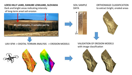
2. Materials and Methods

2.1. Study Site

The study site (47.9807° N, 18.7502° E) comprises a slope in a loess hill land of Ipeľská pahorkatina 20 km north of the Danube river within the Danube Lowlands of Slovakia, Central Europe. The area represents an agriculturally-exploited, hilly loess land that has been exposed to intensive soil erosion (Figure 1). It comprises one cultivated field (58 ha) occupying the entire slope, from a flat plateau to the slightly undulating foot slopes. It is 800 m long, has a mean inclination of 8° and a maximum inclination of 14°.

The altitude ranges between 125 to 220 m above sea level. All the boundaries of this sloping field are constituted by physical landscape features (road, railway, tree alley) that prevent surface water flow from the surroundings. Hence, the study site represents a geomorphological unit in which the entire water flow and erosion/sedimentation cycle are manifested. A shallow, dry periglacial valley diagonally dissects the middle part of the slope.

According to the Koppen–Geiger climate classification, the climate of the area can be classified as Cfb (warm, fully-humid temperate climate with warm summers) with a mean annual temperature of 9.5 °C, mean total annual rainfall 599 mm at the Dudince weather station [34]. Haplic and Luvic Chernozems and Cutanic Luvisols dominate the original soil cover [35]. The loess of bright (yellowish) colour is the prevailing parent material in this area. The high content of carbonates in the loess determines the formation of dark humiferous A horizons for which the soils have a strong colour contrast between topsoil and subsoil. The original soil cover has been intensively transformed by agriculture [36] inducing several degradation processes. The anthropogenically accelerated erosion is the main factor driving soil degradation. Soil surface without vegetation cover (after ploughing, seeding and harvesting) is susceptible to water erosion. Tillage also contributes to overall soil redistribution. These erosion processes transformed the original soils on the slopes into Haplic Calcisols. The major parts of the original, thick, and dark topsoil layer were removed, and their residues were mixed with loess subsoil material by tillage, resulting in poorly-developed A horizons that have a considerably brighter colour than the original soils. Calcisols form brightly coloured areas scattered over the hilly areas of the Danube Lowlands. Dark and bright colours of topsoil create contrasting colour patterns, which are typical for these areas.

The land use in Slovakia underwent significant changes in the 1950s (Figure 1). Until 1949 this area was occupied by a traditional land-use structure comprising narrow strip-fields of small family farms. During the 1950s the agriculture in Slovakia underwent so-called ‘collectivisation’ (i.e., the establishment of cooperative farms), and small fields were merged to form large fields designed for mechanized agriculture. The whole study area was merged into a single large field. It is under a single crop in some years while in other years, it is divided into the upper part (slope and plateau) and the lower part (footslope) with two different crops. The upper part involving the steep slope is used only for densely-seeded crops (cereals). Crop rotation is dominated by winter wheat, maize, oil rape, sunflower and spring barley.

2.2. Methods

2.2.1. Field Survey

The south-eastern (lower) part of the cultivated field, occupying the footslope, is free of erosion patterns, except for the eastern margin, which is situated on a slight terrain step. Morphometric analysis was therefore performed only for the north-western (upper) part of the field. A comparison of the soil erosion patterns and geomorphometric characteristics with detailed soil profile was realized in the area east of the central periglacial valley in the north-western part. The analysed area (27.4 ha) comprises the eastern ridge which was protected by physical boundaries from runoff generated in other areas. In total, 85 pedological hand-auger observations were distributed across the studied area, forming a quasi-regular grid (3 observations per hectare). All observation sites were characterised by field morphological description and basic analytical properties (soil pH, organic carbon, carbonates, and composition of humic substances).

The determination of carbonates was done by the volumetric method using the Janek limemeter, pH_KCl was determined in a soil suspension prepared in a ratio of 1:5 in 1 M KCl, organic and total carbon were determined after dry combustion by elemental analysis, and the composition of humic substances was determined according to [37].

The morphometric properties of the terrain surface in the analysed area were mapped using close-range photogrammetry from an unmanned aerial vehicle (UAV) in September 2019. At the time of the flight, the soil surface was ploughed and without crops. We used a DJI Phantom 4 multicopter with 12.4 megapixels optical sensor for collecting 930 images in natural colour. The average flying height was 115 m above the ground with a vertical view angle of the camera. The side and front overlap ratio of images was 75% and the flight speed was 5 m.s⁻¹. The photographs were processed by the image matching procedure using Agisoft Metashape 1.6.5 software resulting in a 3D point cloud of 33 points/m² on average. Seven ground control points regularly distributed over the mapped area were used to transform the generated 3D point cloud into the common, national S-JTSK coordinate system (European Petroleum Survey Group code 5514). Global Navigation Satellite Systems (GNSS) were used to measure the position of the ground control points (GCPs) with a TOPCON HiPER II GNSS receiver connected to a reference network of the Slovak Observation Service-SKPOS. The GCPs were used for georeferencing the aerial imagery and data products derived from image matching by structure from motion. Point measurements were performed for 30 s using real-time kinematic positioning (RTK) via weighted averaging with an overall accuracy of 1–2 cm. The coordinates of the points were calculated by TopconLink software. The total root mean squared error of georeferencing with the seven points was 8.44 mm. A digital elevation model (DEM) representing the terrain surface (no crops during the flight) was interpolated from the acquired 3D point cloud by the v.surf.rst module in GRASS GIS at the spatial resolution of 1 metre with the following settings: tension = 20, smooth = 0.1, segmax = 40 and npmin = 300.

2.2.2. Detection of Erosion Patterns from Remote Sensing Orthoimagery

The methodology applied at the Bielovce site was based on approaches tested in hilly loess lands of the Danube Lowlands in Slovakia by Fulajtár [30]. The principle is based on the colour differentiation of the soil profile. As indicated earlier, if soils with dark topsoil and pale subsoil are severely eroded, a substantial part of the dark topsoil is removed and a much lighter new A horizon is formed by mixing of the remnants of the original topsoil with the subsoil material having a considerably lighter colour. Thus, the eroded areas have a higher reflectance in the visible part of the spectrum, appearing as bright patterns in comparison with the non-eroded topsoil having a higher humic content. This phenomenon is very typical for hilly lands built by loess deposits in Slovakia.

The erosion patterns at Bielovce were identified using orthorectified natural colour digital aerial photographs in the form of orthophotomosaics. Among several available orthophotomosaics, none showed the entire study area free of crops. Therefore, the two datasets shown in Figure 1 were selected. In the orthophotomosaic from 2002, the lower part of the study area was free of vegetation. In the orthophotomosaic from 2011, the upper part was cultivated without crops. Each part of the study area was interpreted using the orthophotomosaic where the part was free of crops, by the same operator using the same approach, and the results were merged.

Three approaches to erosion pattern delineation were tested: (1) visual interpretation, (2) pixel-based image classification based on soil colour and (3) object-based image classification. The primary purpose of testing different approaches was to explore alternatives to visual interpretation in terms of their complexity and the readability of the outputs. Very few studies have addressed the advantages of object-based over pixel-based classification in erosion mapping, and these are exclusively focused on gully erosion [15,16].

The visual interpretation is a non-automated method in which the erosion patterns are visually identified on-screen by the operator. In the Bielovce area, such identification was based on significant differences in the brightness of strongly-eroded soils compared to the surrounding slightly eroded and non-eroded soils. The areas of erosion patterns were delineated as vector polygons.

Pixel-based image classification is widely used to replace the visual analysis of image data and uses quantitative techniques for automating the identification of features in a scene [38]. This approach typically involves the application of decision rules to each pixel in an image. Decision rules can be extracted automatically from representative sample sites (supervised classification) or by using iterative spectral clustering (unsupervised classification). Other approaches require expert knowledge for the custom specification of decision rules (knowledge-based classification). For the classification of the Bielovce orthophotomosaics, the latest approach was used, which assumed that strongly-eroded regions would appear brighter than slightly eroded and non-eroded regions. The brightness threshold values for distinguishing erosion patterns were determined separately for each utilised orthophotomosaic based on their brightness ranges.

Object-based image classification was developed to overcome the problem of fragmented results generated by the pixel-based classification of high-resolution images [39]. The problem-also known as the salt-and-pepper effect is caused by the categorisation of individual pixels, or a small group of pixels, into different classes from their neighbouring pixels. The object-based approach solves the problem by the creation of a spectrally-homogeneous group of pixels called image objects or segments, followed by the classification of these objects. This approach is similar to human visual interpretation. The resulting patterns are less fragmented and easier to interpret.

The object-based image classification of the Bielovce orthophotomosaics was done using eCognition software. The multi-resolution segmentation implemented in eCognition is superior to other segmentation methods because it allows creating image objects at different hierarchical levels. This approach more realistically reflects the hierarchical nature of objects in the landscape. The multi-resolution segmentation consecutively merges pixels, minimising the average heterogeneity, and maximising the respective homogeneity, of image objects.

To identify soil erosion patterns, two levels of image-objects were created by multi-resolution segmentation. The first level, consisting of larger objects, was designed to classify the main target classes-non-eroded soils, eroded soils, and vegetation cover. It was important to distinguish subtler erosion patterns, with different brightness grades on the upper part of the slope. Therefore, image objects in the 2011 orthophoto were divided into smaller objects, constituting the second hierarchical level.

The second step of object-based image classification required an image object inspection to find the best features for their assignment to the target classes. The classification procedure is based on the assumption that the degree of soil erosion is manifested primarily through the spectral properties of the image objects. Following the pixel-based classification method, brightness values of 170 (2011 orthophoto) and 154 (2002 orthophoto) were used to distinguish between eroded and non-eroded soils. The distinction of bare, non-eroded soil from the land under crop cover could not be achieved via their brightness, as both land cover types appear dark. Therefore, colour expressed by the ratio of green to the overall colour was used instead of brightness. The green ratio threshold value was set to 0.36. In certain parts of the study area, an incorrect assignment of non-eroded soils to eroded soils caused by lighter soil colour was revealed. To solve this problem, the classification was adjusted using the “hue” feature from the Hue Saturation Intensity (HSI) colour transformation. All classification procedure is summarised in

Table 1. The object-based procedure applied to image objects.

Image Object Level 1-Orthophoto 2011
Step	Source Class	Threshold Condition	Target Class
1	unclassified	brightness ≥ 170	eroded soils
2	unclassified	brightness < 170	non-eroded soils
3	non-eroded soils	ratio green > 0.36	vegetation
4	eroded soils	hue < 0.093	non-eroded soils
Image Object Level 1-Orthophoto 2002
Step	Source Class	Threshold Condition	Target Class
1	unclassified	brightness ≥ 154	eroded soils
2	unclassified	brightness < 154	non-eroded soils
3	non-eroded soils	ratio green > 0.36	vegetation
4	eroded soils	brightness < 162 and hue < 0.137	non-eroded soils
Image Object Level 2-orthophoto 2011
Step	Source Class	Threshold Condition	Target Class
1	eroded soils	brightness < 180	slightly eroded soils
2	eroded soils	brightness < 190	moderately eroded soils
3	eroded soils	brightness < 195	strongly eroded soils
4	eroded soils	brightness ≥ 195	very strongly eroded soils

.

2.2.3. Geomorphometric Analysis

The geomorphometric properties of the terrain surface control the action of gravity force on the erosion and deposition of the soil material. Therefore, several parameters were derived to parameterise the effect of terrain morphology using the detailed DEM from close-range photogrammetry. Gravity force F is given by the product of an object’s mass and the magnitude of Earth’s gravitation field. The relationship of the component of gravity force in slope direction F₁ is

F₁ = F sin (β),

(1)

where β = inclination (slope angle).

The mass of concentrated surface water during a rainfall event is proportional to the slope length or contributing area. The simplest estimate of the topographic component of the water erosion potential EP is then

EP ≈ d sin (β) ∨ U sin (β),

(2)

where d = slope length; U = upslope contributing area.

The topographic component of erosion potential can be replaced by the empirically-derived topographic factor LS from the Universal Soil Loss Equation (USLE), which can be calculated thus:

LS = (d/22.13)^m (65.41 sin² (β) + 4.56 sin (β) + 0.065),

(3)

where d = slope length (m); m = 0.5 if the slope angle is 2.86° or more [40].

Slope length was calculated by the r.flow module in GRASS GIS.

The soil erosion and deposition rates can be calculated using the Unit Stream Power-based Erosion/Deposition (USPED) model proposed by [41]. The USPED combines the rainfall erosivity factor R, soil erodability factor K, land cover factor C, the prevention measure factor P of USLE, and the upslope contributing area per unit width U to estimate sediment flow T at sediment transport capacity:

T ≈ RKCPU^m(sin β)ⁿ,

(4)

Exponent m and n control the relative influence of the water and slope terms. The net erosion/deposition ED is estimated as a divergence of sediment flow (change in a two-dimensional vector field representing sediment flow in the direction of elevation surface gradient) T:

$$ED= \frac{\partial (T\cos \propto )}{\partial x}+\frac{\partial (T\sin \propto )}{\partial y}$$

(5)

where α = aspect (direction of elevation surface gradient).

All the erosion factors, except for relief, were quasi-uniform at the study site, and for the calculation of the sediment flow map, the factors R = K = C = P = 1 and exponents m = n = 1 were used. Exponent values close to 1 best reflect the long-term impact of both rill and sheet erosion. Then, the sediment flow T, given by Equation (4), is equal to the topographic component of the water erosion potential EP, given by Equation (2), and the erosion/deposition index ED’ can be calculated by the following Equation (6):

$$ED\prime = \frac{\partial (U\sin \beta \cos \propto )}{\partial x}+\frac{\partial (U\sin \beta \sin \propto )}{\partial y}$$

(6)

The upslope contributing area U was calculated by the r.terraflow module in GRASS GIS. The dominant morphometric variable should be the slope length or contributing area in the landscape with moderate slope angles. One of the major problems of erosion modelling is the uncertainty of the algorithms used for their calculation. If two different algorithms are used, the resulting maps will be different.

3. Results and Discussion

3.1. Verification of Erosion Patterns by Soil Characteristics

Data from all hand-auger observations situated in the brightly coloured areas on the orthoimagery correspond to the eroded soil which can be classified as Haplic Calcisols. In darkly coloured areas, all of the described profiles were Chernozems and Luvisols, sometimes slightly eroded but meeting classification requirements for Chernozems and Luvisols.

The variability of topsoil colour was compared with basic soil characteristics. The results of the bivariate linear regression analysis showed that a high correlation exists between the distribution of CaCO₃ and bright patterns (

Table 2. Summary of bivariate linear regression models between soil sample colour and soil characteristics.

Input Y Range	Lightness of Topsoil Material
Input X Range	CaCO3	Cox	pHKCl	Humic Acids	Fulvid Acids
Observations	85	85	77	77	77
Multiple R	0.81347	0.23349	0.4072	0.44678	0.34898
R2	0.66174	0.05451	0.16581	0.19961	0.12179
Adjusted R2	0.65766	0.04312	0.15469	0.18894	0.11008
Standard Error	2.63945	0.35895	0.0632	0.06191	0.0649
Intercept	0.24646	0.23197	−0.1219	0.37986	0.35711
X Variable (regression slope)	0.01260	0.04449	0.05763	−0.6619	−0.2849
p-value for Intercept	1.03 × 10−51	5.45 × 10−8	0.28026	8.06 × 10−5	3.82 × 10−34
p-value for X Variable	3.11 × 10−21	0.03151	0.00024	4.64 × 10−5	0.0019

). Non-eroded Chernozems and Luvisols have topsoil leached of carbonates. Luvisols have A and B horizon non-calcareous and Chernozems have low carbonate content in A horizons. The C horizons are strongly calcareous. The topsoil layer of brightly coloured areas is rich in CaCO₃ which is mixed into topsoil material from the C horizon by tillage when part of the A horizon is removed by erosion. The carbonate-rich bright patterns have pH much higher than areas with dark soil, but the correlation coefficient of pH values is closer to zero than the CaCO₃ contents in Table 2. Correlation between organic carbon and topsoil colour was weak, which we explain by the high amount of organic matter present in the soils of bright patterns. The major difference is in its quality. Non-eroded land has a more mature darker organic matter than eroded. A more convincing result is shown in the case of humic acids representing a darker, more mature fraction of soil organic matter.

3.2. Interpretation of Orthoimagery

All three tested methods of detecting areal erosion resulted in similar patterns and similar acreage of eroded soils. The patterns delineated by the visual interpretation (Figure 2a) are more generalized than the computer-based methods. However, the smooth boundaries and spatially compact areas from the expert-driven visual delineation make it more suitable for a land management application, e.g., selective fertilizing or cultivation. This approach is, to some extent, subjective because the transition between eroded and non-eroded soils is gradual, while vector polygons delineated by the operator have sharp boundaries. The visual interpretation has limited capability in recognising several levels of land degradation. Usually, only two (maximum three) categories of eroded soils can be distinguished; otherwise, the subjectivity of the interpretation would increase too much.

The pixel-based classification of high-resolution images is a very simple and quick approach but produces scattered patterns, which are less suitable for practical use (Figure 2b). Similarly, to visual interpretation, this method is not suitable for distinguishing more than two classes (eroded and non-eroded soils) because more classes would markedly increase the scatter of the resulting patterns.

The consideration of specific characteristics of image objects, such as shape, texture, or contextual information, in addition to their spectral properties, enables the smoothing, to some extent, of the scattered patterns produced by the pixel-based classification. However, the selection of criteria for object distinction requires much experience. The criteria set for Bielovce caused slightly overestimated total area of the erosion patterns (21.0 ha for object-based classification versus 17.6 ha for visual interpretation and 17.8 for pixel-based classification). The important advantage is that the object-based classification can distinguish several erosion classes (Figure 2d). However, the results of this classification should be verified using field samples. As reported by [29], the spectral differences between slightly eroded and non-eroded soils are very small, and thus the class of non-eroded soils also involve some slightly eroded soils. It is also the case in our studied area. More satisfactory results could be achieved by fuzzy classification or by using hyperspectral data.

The results of the Bielovce study were compared to those of similar studies carried out worldwide, especially in loess areas that experience temperate climates. Existing approaches can be divided into two groups: (1) distinction of bare land from vegetation and (2) distinction of erosion patterns on bare land based on the bright colour of eroded soil. The first approach has been used on non-cultivated land. It is especially successful in arid, tropical, and mountainous areas where the vegetation cover is discontinuous due to harsh environmental conditions. The patches of bare land are exposed to erosional agents. This approach has usually been used for relatively large areas (a few km² to a few thousand km²), and different methods of erosion delineation are used. For example, studies [22,42] identified areas degraded by water erosion, avalanche erosion, and landslides in the Alps, but they only made qualitative assessments and did not delineate any territorial extension of the identified features. Some authors have used visual interpretation; for example, [43,44] employed the traditional visual interpretation of black and white aerial photographs. Various image classification approaches have been the most frequently used [45], and spectral unmixing has also been successful [46].

The second approach, distinguishing bright erosion patterns on bare land, has mainly been used on cultivated land in small study areas (a few tens of ha up to a few km²), and the erosion patterns are delineated either by visual interpretation [31,32,47] or by pixel-based image classification [33]. Some authors tested both approaches and discussed the experience of subjectivity in visual interpretation. Studies based on the distinction of bright patterns on bare land provide much clearer and more detailed maps of eroded soils than the studies based on distinguishing bare land from vegetation cover [48].

The visual interpretation of the historical aerial photograph was made using the same approach as for recent erosion patterns. Numerical processing would likely not improve the result of this task because the fragmentation of the area into small, private fields makes the spectral reflectance too complex. The narrow strip-fields of private farmers represent a very high spatial variability in crop cover. Each small plot has a different crop, and it is improbable to find a period when the majority of the area would be bare with the exposed soil surface, except in winter, but snow or cloudy weather hinder photography. Therefore, the interpretation also has to be done across the fields with crop cover where the erosion patterns are not visible. The boundaries of the eroded areas were extrapolated from the neighbouring bare fields where the erosion patterns were visible. This approach is less accurate as if the soil surface is visible in the imagery, but it is the only way to delineate erosion patterns in areas with such complex land use.

The resulting map (Figure 3) showed that, in 1949, the acreage of strongly-eroded soils reached 10 ha, while in 2011, it was 17.6 ha, which means the eroded area increased by 76%. This significant increase is likely attributable to changed land-use structure and the introduction of mechanized agriculture. The merged large fields have a longer slope. The heavy machinery has increased the ploughing depth and speed, encouraging tillage erosion.

A similar trend of the increasing extent of erosion patterns has been reported from sites in similar hilly loess lands [47,48], but they did not provide quantitative estimations of the increases. [31], working under similar conditions, reported a very high increase in such extension (from 5.2 to 20.2 ha; i.e., 288%).

3.3. The Influence of Terrain Morphology

The LS and ED’ factors, given by Equations (3) and (6), represent geomorphometric factors that control soil loss caused by water erosion. Their isoline fields indicate the spatial distribution of soil erosion rates, and the structure of these fields should be very similar to the real water erosion pattern. At least, very strongly-eroded areas should coincide with certain singularities of the isoline fields of both factors (elevation areas of the mathematical surface of the LS factor and depression areas of the mathematical surface of the ED’ factor). The centroids of those areas should be identical to the positive singular points of the isoline field of the LS factor (summits) and the negative singular points of the isoline field of the ED’ factor (depressions). This argument can be generalised to all erosion models. Bright patterns can thus contribute to erosion model validation. Otherwise, there might be an error in the input morphometric variable settings (slope length, contributing area, etc.) or the analytical forms of the LS and ED’ factors. Moreover, bright patterns on the arable land reflect the cumulative effect of water and tillage erosion. The comparison of the results of several erosion models with the pattern of erosion observed during an extensive field survey conducted in the Kwalei catchment, north-eastern Tanzania showed that the patterns of strongly-eroded areas varied markedly among the models [49].

In the central part of the ridge occurring in the studied area, the isoline field of the LS factor roughly follows the erosion patterns (Figure 4a). A belt of less-eroded soils indicates the structure of the isoline field on the western slope. Also, for this factor, similarly to the ED’ index, it is difficult to explain the occurrence of sharp singularities in the eastern part of the analysed area. However, a singularity should not be the area of the most strongly-eroded soils, but the area of maximal flow velocity (maximal gradient or slope angle). It is a consequence of the similarity between the structure of isoline field of the LS factor and the isoline field of the gradient magnitude or slope angle (exponent m = 0.5 in Equation (3) reduces the effect of increased slope length and slope angle has major control over the LS value). The pattern of the more complex erosion/deposition index ED’ is similar to the LS factor pattern. A comparison of the isoline field of erosion/deposition index ED’ with the erosion pattern (Figure 4b) shows that the most prominent differences exist in the central and lowest parts of the central periglacial valley (values of the contributing area are the highest in the valley). The causality between soil loss and topographic indexes of selected water erosion models was not sufficiently demonstrated (see the summary output of the linear regression in

Table 3. Summary of bivariate linear regression models between soil colour patterns and topographic indexes.

Input Y Range	Topsoil Colour from Figure 1e
Input X Range	First-Order Directional Derivative (Abs Value)	Second-Order Directional Derivative	USLE	USPED	USLE + First-Order Derivative (Abs Value)	USPED + First-Order Derivative (Abs Value)
Observations	4310	4310	4310	4310	4310	4310
Multiple R	0.53477	0.14684	0.39073	0.22613	0.57902	0.57584
R2	0.28597	0.02156	0.15267	0.05113	0.33527	0.33159
Adjusted R2	0.28581	0.02134	0.15247	0.05091	0.33511	0.33144
Standard Error	0.03343	0.00071	4.28632	0.08132	6.43471	0.11692
Intercept	−0.20524	0.00102	−16.045	0.09825	−42.726	−0.714
X Variable	0.38731	−0.00192	33.3083	−0.34559	83.6585	1.50752
p-value for Intercept	<0.001	<0.001	<0.001	<0.001	<0.001	<0.001
p-value for X Variable	<0.001	<0.001	<0.001	<0.001	<0.001	<0.001

).

Also, the impact of tillage erosion on the overall soil loss or accumulation should be considered. The net flux due to tillage translocation after alternating up-or down-slope tillage operations is proportional to the slope gradient (tangent of slope angle). Assuming that tillage erosion can be modelled as a diffusion process, temporal change of altitude, i.e., redistribution of the soil mass, is then proportional to the slope gradient change [50]. Let us consider the elevation profile in the arbitrary tillage direction. The slope of the line tangent to the elevation profile at the given point is proportional to the first-order directional derivative of elevation with respect to the direction of tillage. The change of slope at the given point is proportional to the second-order directional derivative.

Figure 5 shows a large area containing the negative second-order derivatives. All classes of eroded soils are visible. In the case of first-order derivatives, the result is even more convincing. Both sharp positive and less pronounced negative singularity of isoline field is very close to the shape of erosion pattern in western eroded and eastern less eroded part of the field. The brightness of topsoil colour indicating the real erosion positively correlates with the absolute value of the first-order derivative (first column in Table 3). Adding the effect of the USLE or USPED parameter as the weighted water erosion index to the absolute value of the first-order derivative did not improve much the strength of the relationship as the R values indicate (Table 3). Results suggest that either erosion models with the mentioned parameters are inaccurate, or the tillage erosion is currently the dominant erosion process.

Another important factor controlling the spatial distribution of erosion could be the differentiated land use of the past. The steepest parts of the slopes used to be occupied by pastures, while the less steep parts were cultivated. Thus, the steepest slopes could be more protected by vegetation in the past, and thus less eroded than the less steep slopes.

Studies of the relief impact on erosion have tested various morphometric characteristics, such as the LS factor of the USLE and the topographic factor based on the unit stream power [51], topographic index of susceptibility for water erosion [52], and many others. Several studies were also carried out in environments similar to the Bielovce Site. For example, [53] examined the slope, plan curvature, topographic wetness index, and sediment transport index, and [33] investigated the slope, profile curvature, tangential curvature, geometric forms, and upslope contributing area. The results identified some relation of erosion patterns to relief. However, the correlations between the erosion patterns and the particular morphometric characteristics were usually weak. The relation between relief and erosion is very complex and overlaps with the impacts of other factors.

4. Conclusions

The combined use the field soil observation data, interpretation of historical aerial orthophotomosaic, image matching and geomorphometric analyses in GIS of the study area in the loess hill land of the Danube Lowland provided means for assessing the spatial distribution and temporal dynamics of soil erosion. All three tested approaches of erosion identification from remote sensing data achieved acceptable results, indicating advantages and limitations:

• Visual interpretation can benefit from the experience of an operator who can assess the erosion features in a more comprehensive way than can a mathematical algorithm. It is important, especially in processing historical aerial photographs, as their land-use structure can be too complex for image classification methods. The major advantage of this approach is that the resulting erosion patterns are smoother and less scattered than those of image classification methods, so the resulting maps are more suitable for practical as applications in land management and conservation. The disadvantages comprise a high labour demand and subjectivity of interpretation, which typically distinguish up to three categories.
• Image classification is less subjective. If quantitative classification criteria are used, the results can be more quickly compared to those of other studies. Quantitative classes allow for distinguishing several levels of soil degradation.
• Contrary to improved accuracy, a disadvantage of the pixel-based classification is the scattered pattern of the resulting class of eroded soils.
• Object-based classification results in more realistic, larger, and smoother patterns and it also distinguishes the transitional categories of moderately-eroded soils more precisely.

The maps created by all three methods are far more precise than the maps based on a conventional survey without the use of remote sensing.

Valuable information was gained from a comparison of historical and recent aerial photographs. This approach can be used for the assessment of the long-term development of erosion patterns.

Investigating the relationship between relief and the spatial distribution of eroded soils showed that the eroded soils occupy steep parts of the slopes. However, correlations of the individually-tested relief parameters were loose, indicating that the impact of relief morphology on erosion is complex. The simple topographic parameters used in the tested erosion models did not sufficiently express the real complexity of the influence of relief. The main problem is that these parameters are not based on all factors which enrol all erosion processes. Therefore, they cannot fully express the spatial relation between total erosion and topography. The impact of the terrain morphology is different for water erosion and tillage erosion. The direction of water flow is not always the same as the direction of tillage. Summing the results of the tillage erosion model and water erosion model may not be the best solution. More complex erosion models need to be developed to express the synergy effects of tillage erosion and water erosion. The investigation of bright soil patterns on arable land by image interpretation methods provides a valuable platform for validating the synergy effects.

References

1. De Vente, J.; Posen, J.; Verstraeten, G.; Govers, G.; Vanmaercke, M.; Van Rompaey, A.; Arabkhedri, M.; Boix-Fayos, C. Predicting soil erosion and sediment yield at regional scales: Where do we stand? Earth Sci. Rev. 2013, 127, 16–29. [Google Scholar] [CrossRef]
2. Bosco, C.; de Rigo, D.; Dewitte, O.; Poesen, J.; Panagos, P.; Arabkhedri, M.; Boix-Fayos, C. Modelling soil erosion at European scale: Towards harmonization and reproducibility. Nat. Hazards Earth Syst. Sci. 2015, 15, 225–245. [Google Scholar] [CrossRef] [Green Version]
3. Borrelli, P.; Paustian, K.; Panagos, P.; Jones, A.; Schütt, B.; Lugato, E. Effect of Good Agricultural And Environmental Conditions on erosion and soil organic carbon balance: A national case. Land Use Policy 2016, 50, 408–421. [Google Scholar] [CrossRef]
4. Vrieling, A. Satellite remote sensing for water erosion assessment: A review. Catena 2006, 65, 2–18. [Google Scholar] [CrossRef]
5. Ben-Dor, E.; Inbar, Y.; Chen, Y. The reflectance spectra of organic matter in the visible near-infrared and short wave infrared region (400–2500 nm) during a controlled decomposition proces. Remote Sens. Environ. 1997, 61, 1–15. [Google Scholar] [CrossRef]
6. Boardman, J. The value of Google EarthTM for erosion mapping. Catena 2016, 143, 123–127. [Google Scholar] [CrossRef]
7. Pereira, P.; Brevik, E.C.; Munoz-Royas, M.; Miller, B.A. Soil Mapping and Process Modeling for Sustainable Land Use Management; Elsevier: Amsterdam, The Netherlands, 2017. [Google Scholar]
8. Wulf, H.; Mulder, T.; Schaepman, M.E.; Keller, A.; Jörg, P. Remote Sensing of Soils, NPOC/INRA; University of Zurich, Remote Sensing Laboratories: Zurich, Switzerland, 2015. [Google Scholar]
9. Li, M.; Zang, S.; Zhang, B.; Li, S.; Wu, C. A review of remote sensing image classification techniques: The role of spatio-contextual information. Eur. J. Remote Sens. 2014, 47, 389–411. [Google Scholar] [CrossRef]
10. Liu, H.; Hormann, G.; Qi, B.; Yue, Q. Using high-resolution aerial images to study gully development at the regional scale in southern China. Int. Soil Water Conserv. Res. 2020, 8, 173–184. [Google Scholar] [CrossRef]
11. Wang, B.; Zhang, Z.; Wang, X.; Zhao, X.; Yi, L.; Hu, S. Object-based mapping of gullies using optical images: A case study in the black soil region, Northeast of China. Remote Sens. 2020, 12, 487. [Google Scholar] [CrossRef] [Green Version]
12. Bouaziz, M.; Wijaya, A.; Gloaguen, R. Remote gully erosion mapping using ASTER data and geomorphologic analysis in the Main Ethiopian Rift. Geo Spat. Inf. Sci. 2011, 14, 246–254. [Google Scholar] [CrossRef]
13. Shruthi, R.B.V.; Kerle, N.; Jetten, V. Object-based gully feature extraction using high spatial resolution imagery. Geomorphology 2011, 134, 260–268. [Google Scholar] [CrossRef]
14. D’Oleire-Oltmanns, S.; Marzolff, I.; Tiede, D.; Blaschke, T. Detection of gully-affected areas by applying object-based image analysis (obia) in the region of Taroudannt, Morocco. Remote Sens. 2014, 6, 8287–8309. [Google Scholar] [CrossRef] [Green Version]
15. Shahabi, H.; Jarihani, B.; Piralilou, S.T.; Chittleborough, D.; Avand, M.; Ghorbanzadeh, O. A semi-automated object-based gully networksdetection using different machine learning models: A case study of Bowen catchment, Queensland, Australia. Sensors 2019, 19, 4893. [Google Scholar] [CrossRef] [PubMed] [Green Version]
16. Karami, A.; Khoorani, A.; Nuhegar, A.; Shamsi, S.R.F.; Moosavi, V. Gully erosion mapping using object-based and pixel-based image classification methods. Environ. Eng. Geosci. 2015, 21, 101–110. [Google Scholar] [CrossRef]
17. Brodský, L.; Vašát, R.; Klement, A.; Zádorová, T.; Jakšík, O. Uncertainty propagation in VNIR reflectance spectroscopy soil organic carbon mapping. Geoderma 2013, 199, 54–63. [Google Scholar] [CrossRef]
18. Mirzaee, S.; Ghorbani-Dashtaki, S.; Mohammadi, J.; Asadi, H.; Asadzadeh, F. Spatial variability of soil organic matter using remote sensing data. Catena 2016, 145, 118–127. [Google Scholar] [CrossRef]
19. Wang, X.; Zhang, F.; Kung, H.; Johnson, V.C. New methods for improving the remote sensing estimation of soil organic matter content (SOMC) in the Ebinur Lake Wetland National Nature Reserve (ELWNNR) in northwest China. Remote Sens. Environ. 2018, 218, 104–118. [Google Scholar] [CrossRef]
20. Angelopoulou, T.; Tziolas, N.; Balafoutis, A.; Zalidis, G.; Bochtis, D. Remote sensing techniques for soil organic carbon estimation: A review. Remote Sens. 2019, 11, 676. [Google Scholar] [CrossRef] [Green Version]
21. Luleva, M.I.; Van Der Werff, H.; Van Der Meer, F.; Jetten, V. Gaps and opportunities in the use of remote sensing for soil erosion. Chem. Bulg. J. Sci. Educ. 2012, 21, 748–764. [Google Scholar]
22. Meusburger, K.; Konz, N.; Schaub, M.; Alewell, C. Soil erosion modelled with USLE and PESERA using QuickBird derived vegetation parameters in an alpine catchment. Int. J. Appl. Earth Obs. Geoinf. 2010, 12, 208–215. [Google Scholar] [CrossRef]
23. Chabrillat, S.; Milewski, R.; Schmid, T.; Rodriguez, M.; Escribano, P.; Pelayo, M.; Palacios-Orueta, A. Potential of hyperspectral imagery for the spatial assessment of soil erosion stages in agricultural semi-arid Spain at different scales. In Proceedeings of the 2014 IEEE Geoscience and Remote Sensing Symposium, Quebec, QC, Canada, 13–18 July 2014; pp. 2918–2921. [Google Scholar]
24. Mathieu, R.; Cervelle, B.; Rémy, D.; Pouget, M. Field-based and spectral indicators for soil erosion mapping in semi-arid mediterranean environments (Coastal Cordillera of central Chile). Earth Surf. Process. Landf. 2006, 32, 13–31. [Google Scholar] [CrossRef]
25. Zhang, X.; Dou, X.; Xie, Y.; Liu, H.; Wang, N.; Wang, X.; Pan, Y. Remote sensing inversion model of soil organic matter in farmland by introducing temporal information. Trans. Chin. Soc. Agric. Eng. 2018, 34, 143–150. [Google Scholar]
26. Lin, C.; Zhou, S.; Wu, S.; Zhu, Q.; Dang, Q. Spectral response of different eroded soils in subtropical China: A case study in Changting county, China. J. Mt. Sci. 2014, 11, 697–707. [Google Scholar] [CrossRef]
27. Sepuru, T.K.; Dube, T. An appraisal on the progress of remote sensing applications in soil erosion mapping and monitoring. Remote Sens. Appl. Soc. Environ. 2017, 9, 1–9. [Google Scholar] [CrossRef]
28. Žížala, D.; Zádorová, T.; Kapička, J. Assessment of soil degradation by erosion based on analysis of soil properties using aerial hyperspectral images and ancillary data, Czech Republic. Remote Sens. 2017, 9, 28. [Google Scholar] [CrossRef] [Green Version]
29. Žížala, D.; Juřicová, A.; Zádorová, T.; Zelenková, K.; Minařík, R. Mapping soil degradation using remote sensing data and ancillary data: South-East Moravia, Czech Republic. Eur. J. Remote Sens. 2019, 52 (Suppl. 1), 108–122. [Google Scholar] [CrossRef] [Green Version]
30. Fulajtár, E. Identification of severely eroded soils from remote sensing data tested in Rišňovce, Slovakia. In Sustaining the Global Farm. Proceedings of the 10th International Soil Conservation Organization Meeting held May 24–29, 1999, West Lafayette, IN, USA; Stott, D.E., Mohtar, R.H., Steinardt, G.C., Eds.; International Soil Conservation Organization in cooperation with USDA and Purdue University: West Lafayette, IN, USA, 2001; pp. 1075–1082. [Google Scholar]
31. Smetanová, A.; Kožuch, M.; Čerňanský, J. The land use changes in 20th century and their geomorphological implications in a lowland agricultural area (Voderady, Trnavská tabuľa Table Plain, Slovakia). Geomorphol. Slovaca Bohem. 2009, 9, 57–63. [Google Scholar]
32. Smetanová, A. Bright patches on chernozems and their relationship to the relief. Geogr. Cas. 2009, 61, 215–227. [Google Scholar]
33. Fulajtár, E.; Jenčo, M.; Saksa, M. Soil erosion mapping with the aid of aerial photographs tested at Pastovce, Ipe’ská pahorkatina. In Interdisciplinary Studies of River Channels and UAV Mapping in the V4 Region; Šulc Michalková, M., Miřijovský, J., Eds.; Comenius University: Bratislava, Slovakia, 2016; pp. 247–268. [Google Scholar]
34. Kottek, M.; Grieser, J.; Beck, C.; Rudolf, B.; Rubel, F. World Map of the Köppen-Geiger climate classification updated. Meteorol. Z. 2006, 15, 259–263. [Google Scholar] [CrossRef]
35. IUSS Working Group WRB. World Reference Base for Soil Resources 2014, Update 2015. International Soil Classification System for Naming Soils and Creating Legends for Soil Maps; World Soil Resources Report No. 106; FAO: Rome, Italy, 2014. [Google Scholar]
36. Stankoviansky, M.; Fulajtár, E.; Jambor, P. Slovakia. In Soil Erosion in Europe; Boardman, J., Poesen, J., Eds.; John Wiley & Sons, Ltd.: Chichester, UK, 2006; pp. 117–138. [Google Scholar]
37. Fiala, K.; Barančíková, G.; Brečková, V.; Búrik, V.; Houšková, B.; Chomaničová, A.; Kobza, J.; Litavec, T.; Makovníková, J.; Matúšková, L.; et al. Záväzné metódy rozborov pôd. Čiastkový monitorovací systém-Pôda. (Binding Methods of Soil Analysis. Partial Monitoring System-Soil); Výskumný ústav pôdoznalectva a ochrany pôdy: Bratislava, Slovakia, 1999. [Google Scholar]
38. Lillesand, T.M.; Kiefer, R.W.; Chipman, J.W. Remote Sensing and Image Interpretation, 7th ed.; John Wiley & Sons, Ltd.: Chichester, UK, 2015. [Google Scholar]
39. Blaschke, T.; Lang, S.; Hay, G. Object-Based Image Analysis; Springer: Berlin, Germany, 2008. [Google Scholar]
40. Wischmeier, W.H.; Smith, D.D. Predicting rainfall erosion losses—A guide to conservation planning. In USA Agriculture Handbook No. 537; U.S. Department of Agriculture: Washington, DC, USA, 1978. [Google Scholar]
41. Mitasova, H.; Mitas, L. Multiscale soil erosion simulations for land use management. In Landscape Erosion and Landscape Evolution Modelling; Harmon, R.S., Doe, W.W., Eds.; Kluwer Academic/Plenum Publishers: New York, NY, USA, 2001; pp. 321–347. [Google Scholar]
42. Alewell, C.; Meusburger, K.; Brodbeck, M.; Bänninger, D. Methods to describe and predict soil erosion in mountain regions. Landsc. Urban Plan. 2008, 88, 46–53. [Google Scholar] [CrossRef]
43. Fadul, H.M.; Salih, A.A.; Ali, I.A.; Inanaga, S. Use of remote sensing to map gully erosion along the Atbara River, Sudan. Int. J. Appl. Earth Obs. Geoinf. 1999, 1, 175–180. [Google Scholar] [CrossRef]
44. Servenay, A.; Prat, C. Erosion extension of indurated volcanic soils of Mexico by aerial photographs and remote sensing analysis. Geoderma 2003, 117, 367–375. [Google Scholar] [CrossRef]
45. Bouaziz, M.; Leidig, M.; Gloaguen, R. Optimal parameter selection for qualitative regional erosion risk monitoring: A remote sensing study of SE Ethiopia. Geosci. Front. 2011, 2, 237–245. [Google Scholar] [CrossRef] [Green Version]
46. De Jong, S.M.; Paracchini, M.L.; Bertolo, F.; Folving, S.; Megier, J.; de Roo, A.P.J. Regional assessment of soil erosion using the distributed model SEMMED and remotely sensed data. Catena 1999, 37, 291–308. [Google Scholar] [CrossRef]
47. Báčová, M.; Krása, J. Application of historical and recent aerial imagery in monitoring water erosion occurrences in Czech highlands. Soil Water Res. 2016, 11, 267–276. [Google Scholar] [CrossRef] [Green Version]
48. Šarapatka, B.; Netopil, P. Erosion processes on intensively farmed land in the Czech Republic: Comparison of alternative research methods. In Proceedings of the 19th World Congress of Soil Science, Soil Solutions for a Changing World, Brisbane, Australia, 1–6 August 2010. [Google Scholar]
49. Vigiak, O.; van Loon, E.; Sterk, G. Modelling spatial scales of water erosion in the West Usambara Mountains of Tanzania. Geomorphology 2006, 76, 26–42. [Google Scholar] [CrossRef]
50. Govers, G.; Vandaele, K.; Desmet, P.; Poesen, J.; Bunte, K. The role of tillage in soil redistribution on hillslopes. Eur. J. Soil Sci. 1994, 45, 469–478. [Google Scholar] [CrossRef]
51. Mitasova, H.; Hofierka, J.; Zlocha, M.; Iverson, L.R. Modelling topographic potential for erosion and deposition using GIS. Int. J. Geogr. Inf. Syst. 1996, 10, 629–641. [Google Scholar] [CrossRef]
52. Chappell, A. Modelling the spatial variation of processes in the redistribution of soil: Digital terrain models and 137Cs in southwest Niger. Geomorphology 1996, 17, 249–261. [Google Scholar] [CrossRef]
53. Zádorová, T.; Žížala, D.; Penížek, V.; Čejková, Š. Relating extent of colluvial soils to topographic derivatives and soil variables in a Luvisol sub-catchment, Central Bohemia, Czech Republic. Soil Water Res. 2014, 9, 47–57. [Google Scholar] [CrossRef] [Green Version]
Figure 1. Study site: (a) location; (b) soil cover (original Chernozem (A), eroded Calcisol (B) and bright eroded patterns (C)); land-use structure in 1949 (c), 2002 (d) and 2011 (e) with 5 m contour interval.
Remotesensing 12 04047 g001
Figure 2. Comparison of erosion patterns obtained by different methods: visual interpretation (a), pixel-based classification (b), object-based classification (c) with two erosion categories and (d) with five erosion categories used for comparison with the modelled erosion patterns.
Remotesensing 12 04047 g002
Figure 3. Increase in erosion areas from 1949 to 2002/2011.
Remotesensing 12 04047 g003
Figure 4. Isoline field: topographic factor LS (a), erosion/deposition index ED’ (b). Each parameter is expressed by two figures, the left image showing the isoline field and the right image showing the overlay of the isoline field and erosion pattern obtained by object-based classification.
Remotesensing 12 04047 g004aRemotesensing 12 04047 g004b
Figure 5. Overlay of the isoline field of the first-order (left image) and the second-order (right image) partial derivative of elevation with respect to past prevailing tillage direction displayed in Figure 1c compared with the erosion pattern obtained by object-based classification (background map).
Remotesensing 12 04047 g005