Characteristic Analysis and Indexing of Multimachine Transient Stabilization Using Virtual Synchronous Generator Control

Abstract

As distributed power sources via grid-connected inverters equipped with functions to support system stabilization are being rapidly introduced, individual systems are becoming more complex, making the quantification and evaluation of the stabilizing functions difficult. Therefore, to introduce distributed power sources and achieve stable system operation, a system should be reduced to a necessary but sufficient size in order to enable the quantification of its behavior supported by transient theory. In this study, a system in which multiple distributed power supplies equipped with virtual synchronous generator control are connected is contracted to a two-machine system: a main power supply and all other power supplies. The mechanical torque of each power supply is mathematically decomposed into inertia, damping, synchronization torques, and the governor effect. The system frequency deviations determined by these elements are quantitatively indexed using MATLAB/Simulink. The quantification index displayed in three-dimensioned graphs illustrates the relationships between the various equipment constants of the main power supply, the control variables of the grid-connected inverter control, and the transient time series. Moreover, a stability analysis is performed in both the time and frequency domains.

1. Introduction

Conventional power systems use synchronous generators as their main power source, the swing characteristics of which suppress the power system swing owing to the load power and generated power fluctuations [1]. However, due to recent advancements in distributed power sources, such as renewable energy, a large number of grid-connected inverters are being connected to power systems. The inertial power of the entire system, which generally suppresses the fluctuations of the power system, is insufficient when the capacity of the grid-connected inverters exceeds the capacity of the main power supply, making it challenging to maintain stability [2,3]. There is thus a need for the grid-connected inverters of distributed power sources to have power generation functionality and to suppress the fluctuations of the power system [4]. Obviously, it is necessary to address other existing technical issues such as the intermittentness of solar energy [5], limitations on the data capacity of smart grids [6], the influence of power electronics equipment on power quality [7], and the effectiveness of energy trading; various studies have investigated these issues [8]. Although the problem of the capacity of grid-connected inverters exceeding that of the main power supply was previously regarded as being characteristic of microgrids (MGs), a similar problem has recently been identified in large-scale smart grids. Field research using actual data is therefore being actively conducted (in Korea [9], Canada [10], Oahu, HI [11,12,13], and the USA in general [14]). To leverage open-source system validation platforms (SVPs) for interoperable test procedures, research using power/controller hardware-in-the-loop (PHIL/CHIL) is also being actively promoted [15,16,17,18]; Ref. [19] summarizes these trends.

So-called “smart inverters” for photovoltaic power generation in detached houses have a functionality that can contribute to maintaining the balance between electricity supply and demand at steady state [20,21]. Some smart inverters realize grid-support functions (GSFs) based on power control according to the communication of commands at a higher level of integrated control, in which case it is relatively easy to estimate the effects and formulate the required specifications. In contrast, some inverters autonomously calculate the power imbalance of the system without higher-level control commands, in a manner similar to that of synchronous generators, immediately after fluctuations in the load/generated power. In this way, high-performance grid-connected inverters can control their own inputs and outputs using high responsiveness, which has been attracting increased attention. The autonomous functions are generally installed in the primary control unit of the inverter, and the details are rarely disclosed by manufacturers. It is therefore difficult to estimate their effects and formulate the required specifications [22]. A protocol study was conducted to comprehensively test the capability of smart inverters to stabilize MGs [23,24]. Reference [24] examines various testing methods using three commercially available, single-phase, residential-scale photovoltaic (PV) inverters from three different manufacturers. In [23], a test protocol for smart inverters that can utilize battery energy storage systems is studied, and a summary is provided of issues related to four interoperability function tests defined in IEC TR 61850-90-7: the specified active power test (INV4), the var-priority volt-var test (VV), the specified power factor test (INV3), and frequency-watt control (FW) from storage.

Research on optimizing parameter settings to improve the performance of distribution systems by making smart inverters compatible with volt-var and volt-watt functions is in progress [9,14,25,26,27,28,29]. It has been proposed that if the volt-watt function is prioritized over the volt-var function, the system voltage will vibrate continuously [27]. Conversely, when suppressing the volt-watt function, fairness is required to reduce the amount of power generated by distributed power sources (PVs, etc.) [29]. To establish a method for handling these problems, the simulation analysis of an actual field is required: an analysis using actual data in an actual feeder [9,14], quasi-static time series simulation using an open distribution system simulator (OpenDSS) [9], and HIL simulation [29] have been reported thus far. Moreover, in [26], the effects of improved volt-var control using the particle swarm optimization (PSO) algorithm on line loss and operation cost reduction are demonstrated, and in [25,28], the optimum utilization of PV inverter capacity is described.

Some smart inverters obtain the same characteristics by simultaneously mimicking the swing and excitation characteristics of a synchronous generator [30,31,32,33], while others obtain similar characteristics without focusing on the excitation characteristics [34,35]. Unfortunately, there is little research on volt-var, volt-watt, and frequency-watt control that focuses on transient responses related to the swing characteristics of synchronous generators. Although the GSFs of frequency-watt controls between grid-forming and grid-following PV inverters are discussed in [12], the transient response, which corresponds to the inertial response, has not been discussed. However, research on improving transient responses with inverters is ongoing [35,36,37,38,39,40]. References [38,39,40] propose an improved GSF by using the direct current (DC) energy buffer of a grid-connected inverter. In [40], a new distributed consensus-based control that reduces the circulating power between parallel running inverters is demonstrated. In [39], experimental results that achieve an inertial response by connecting only a small capacitor to the DC link part are presented. Reference [37] presents the experimental results for a decentralized control that controls multiple PV inverters as master/slave without using a storage battery. In [38], a control that achieves both a droop response and an inertial response using a hybrid energy storage system (ESS) and that reduces the deterioration of the battery storage by using a super capacitor is proposed. A method that strictly simulates the swing characteristics of a synchronous generator using battery power is called virtual synchronous generator (VSG) control, and many studies have been conducted to improve this method [30,31]. For example, reference [35] presents the prediction model of a VSG to enhance suppression performance of the voltage and frequency variations. In [36], a method for adding a phase adjustment function to multi-loop VSG control was introduced, and it was reported that renewable energy-based inverters were used in a plug-and-play manner to reduce the harmonics and oscillation and to improve the dynamic response and power quality.

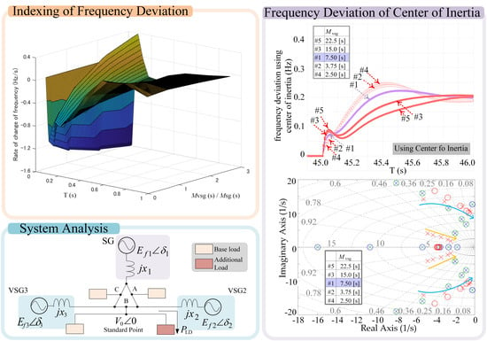
The swing characteristics of the synchronous generator to be mimicked in this study are determined to be the characteristics of the rotor, expressed by both the inertial and damping responses. The response attributed to the synchronization force is added when multiple synchronous machines are interconnected [41]. After some time, the control of the governor becomes effective, and a governor-free response is added to the inertial and damping responses [42]. The deviation of the system frequency represents the difference between the electrical angular velocity and rated angular velocity of the rotor reference, which is equal to the deviation of the internal phase difference angle (angular velocity). That is, to accurately analyze the transient fluctuation of the system frequency, it is essential to evaluate the inertial effect, damping effect, synchronization effect, governor effect, etc. separately from the swing equation of the generator rotor angle (mechanical angle). Nevertheless, few studies have analyzed the system frequency by separating and analyzing the components of the swing equation of the generator rotor in detail. Therefore, in this study, the swing characteristics of the generator mimicked by the grid-connected inverter are accurately separated by effect, and the correlation between each effect and the values of the control parameters is clarified. The mechanical torque of each power supply, which is calculated mathematically, is decomposed into inertia, damping, synchronization torque, and governor effect, and the decomposition components were analyzed and indexed from both time and frequency domains. This provides an indicator of the parameter settings required for grid-connected inverters not only in MGs but also large smart grids. To acquire the time-series data that is used to decompose the above-mentioned mechanical torque, the Institution of Electrical and Electronic Engineers (IEEE) 9 bus model is adopted, and two distributed power sources are connected to the existing power system through a grid-connected inverter. Although simulation results are to be verified separately, it should be noted that it is not theoretically necessary to be limited to IEEE 9 bus from the viewpoint of reducing multiple machines to a two-machine model. The transient characteristics are analyzed using numerical simulation results from MATLAB/Simulink according to a mathematical model, and the correlation between each control parameter and each response is clarified based on the concept of the center of inertial frequency. In this system, a synchronous generator is the main power source. The two inverters are reduced to one, and each is equipped with the same VSG control. The total capacities of the grid-connected inverters are assumed to be almost the same as that of the main power supply, thereby making it difficult to maintain system stability. That is, the multi-machine large-scale system was reduced to a two-machine model. This not only reduces the mathematical analysis associated with a multi-machine model but also allows analysis that can be focused on various parameter ratios between the conventional main power supply and other distributed power sources.

The structure of this study is as follows: Section 2 reviews the interconnection principle of multiple synchronous machines, and Section 3 analyzes the transient response characteristics from simulation test results in response to changes in each parameter of the VSG control inverter. The frequency of the center of inertia is also calculated in Section 3, while Section 4 discusses indicators for the VSG inverter based on the outcomes of the torque response and the center of inertia in both the time and frequency domains. Section 5 summarizes this study.

2. Theory of Multiple Synchronous Machine Interconnections

2.1. Synchronous Generator Model

Figure 1 is based on the swing equation for a synchronous generator (SG) (Equation (1)) [41]:

$$\Delta P=\frac{M}{{\omega }_0}{s}^2\delta +\frac{1}{{\omega }_0}\left(D+\frac{1/R}{1+sT}\right)s\delta +K\delta$$

(1)

where s is the Laplacian differential operator, $\Delta P$ [pu] is the machine input torque, $\delta$ [rad] is the phase difference angle, and ${\omega }_0$ [rad/s] is the rated angular velocity. Because these are all considered on the basis of 1 pu, $\Delta P$ can be thought of as the fluctuation of the input/output power. $M$ [s] is the unit inertia constant, $D$ [pu/pu] is the dumping coefficient, and $R$ [pu/pu] and $T$ [s] are the droop and time constants related to the active power and system frequency of the governor, respectively. $K$ [pu/rad] is the synchronization coefficient. The transfer function of the governor in the SG is set to be $H_{\mathrm{sg}}(s)$, and the transfer function from the input/output power fluctuation $\Delta P$ to the frequency deviation (slip) $\Delta \omega$ [pu] in a stand-alone SG was set to $G_{\mathrm{sg}}(s)$.

In the case of a conventional SG, the governor time constant $T$ [s] is several hundreds of milliseconds, and its effect appears after the delay from the onset of the fluctuation in the input/output power. The synchronization torque term $K\delta$ is relevant when the SG is connected to another synchronous machine, and the synchronization coefficient $K$ [pu/rad] is determined by the interconnection style (bus model). Therefore, assuming that the governor response is not on time, the transfer function $G_{\mathrm{sg}}(s)$ in a stand-alone SG immediately after the onset of input/output power fluctuations is only determined by the inertial torque term $(M/{\omega }_0)s^2\delta$ and the dumping torque term $(D/{\omega }_0)s\delta$.

The synchronous machine block, a device in the standard library of Simscape Electrical in the MATLAB/Simulink environment, is used for the governor model $H_{\mathrm{sg}}(s)$, for which Equation (1) holds. A model of a general excitation system is also included, but details are omitted here because the swing equation is the focus of this study.

2.2. Virtual Synchronous Generator Control Model

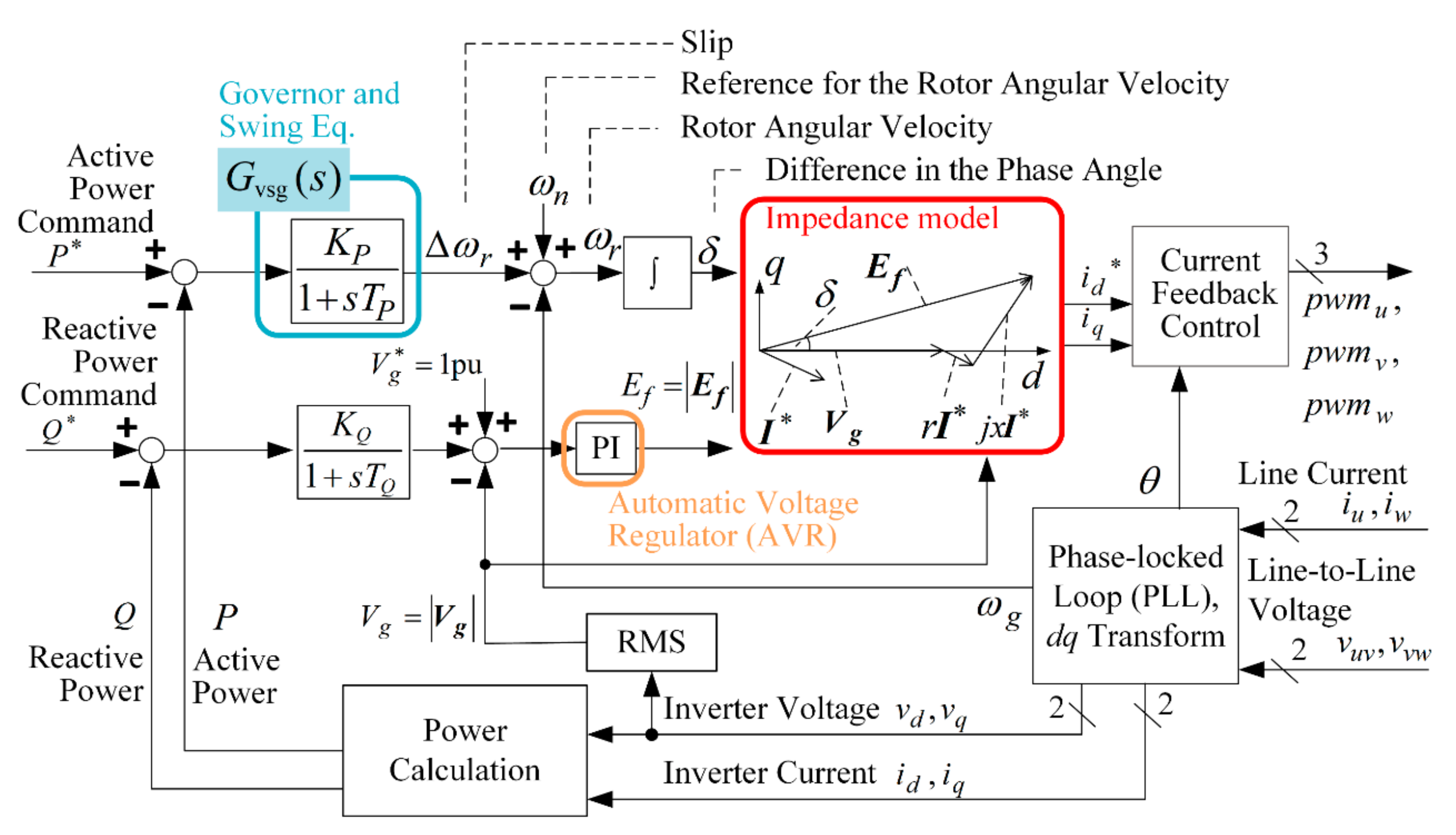
Figure 2 shows a block diagram of a VSG control installed in a grid-connected inverter control. A Kawasaki VSG [30,31] is used in this study. The transfer function $G_{\mathrm{vsg}}(s)$ enclosed by the light-blue frame in Figure 2 corresponds to $G_{\mathrm{sg}}(s)$ in Figure 1. Because the time required for the fuel injection and delay in the electrical system do not need to be considered in the governor simulated according to VSG control, the governor time constant $T$ [s] in Figure 1 is 0 s, and $G_{\mathrm{vsg}}(s)$ expresses the combination of the governor model with a delay time of zero and the inertial torque term. $K_P$ [pu/pu] is the droop related to the active power $P$ [pu] and angular frequency $\omega$ [pu] of the terminal voltage estimated from the phase-locked loop (PLL). $M_P$ [s] is the unit inertia constant of the VSG, $T_P=M_P{K}_P$ [s] is the time constant needed for inertial simulations, and the angular frequency deviation (slip) $\Delta \omega$ [pu] and internal phase difference $\delta$ [rad] can be calculated in the same way as for the SG.

The magnitude of the generator (induced) voltage vector $E_f=\left|{\mathit{E}}_f\right|$ [pu] is determined from the relationship between the reactive power and terminal voltage. $K_Q$ [pu/pu] is the droop associated with the reactive power $Q$ [pu], and the magnitude of the terminal (inverter) voltage vector is $V_g=\left|{\mathit{V}}_g\right|$ [pu]. $T_Q$ [s] is the filter time constant, and the conventional proportional-integral (PI) compensator is used as the AVR.

The vector diagram enclosed in the red frame in Figure 2 is the impedance model, which illustrates the relationship between the generator voltage vector ${\mathit{E}}_f$, terminal voltage vector ${\mathit{V}}_g$, command value vector ${\mathit{I}}^{*}$ of the inverter current, and impedance $r$, $x$ [pu]. The impedance $r$, $x$ [pu] is a pseudo-impedance set in the VSG control software, and it becomes dominant over the alternating current (AC) output filter impedance in low-frequency regions, such as commercial frequencies. The ratio of the virtual inductance $x$ and virtual resistance $r$ is empirically set to $x=2r$. The current command vector value ${\mathit{I}}^{*}$ is expressed by Equation (2) [30,31], as a vector of the dq coordinates:

$${\mathit{I}}^{*}=\left[\begin{array}{c}{i}_d^{*}\\ i_q^{*}\end{array}\right]=\frac{1}{r^2+x^2}\left[\begin{array}{cc}r& x\\ -x& r\end{array}\right]\hspace{0.17em}\left(\left[\begin{array}{c}{e}_d\\ e_q\end{array}\right]-\left[\begin{array}{c}{v}_d\\ v_q\end{array}\right]\right).$$

(2)

2.3. System Model

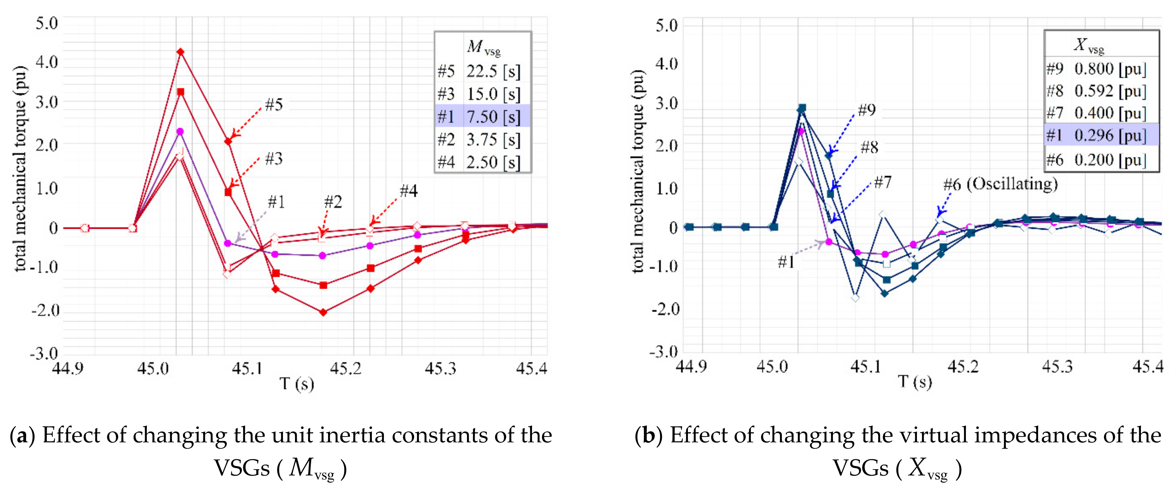
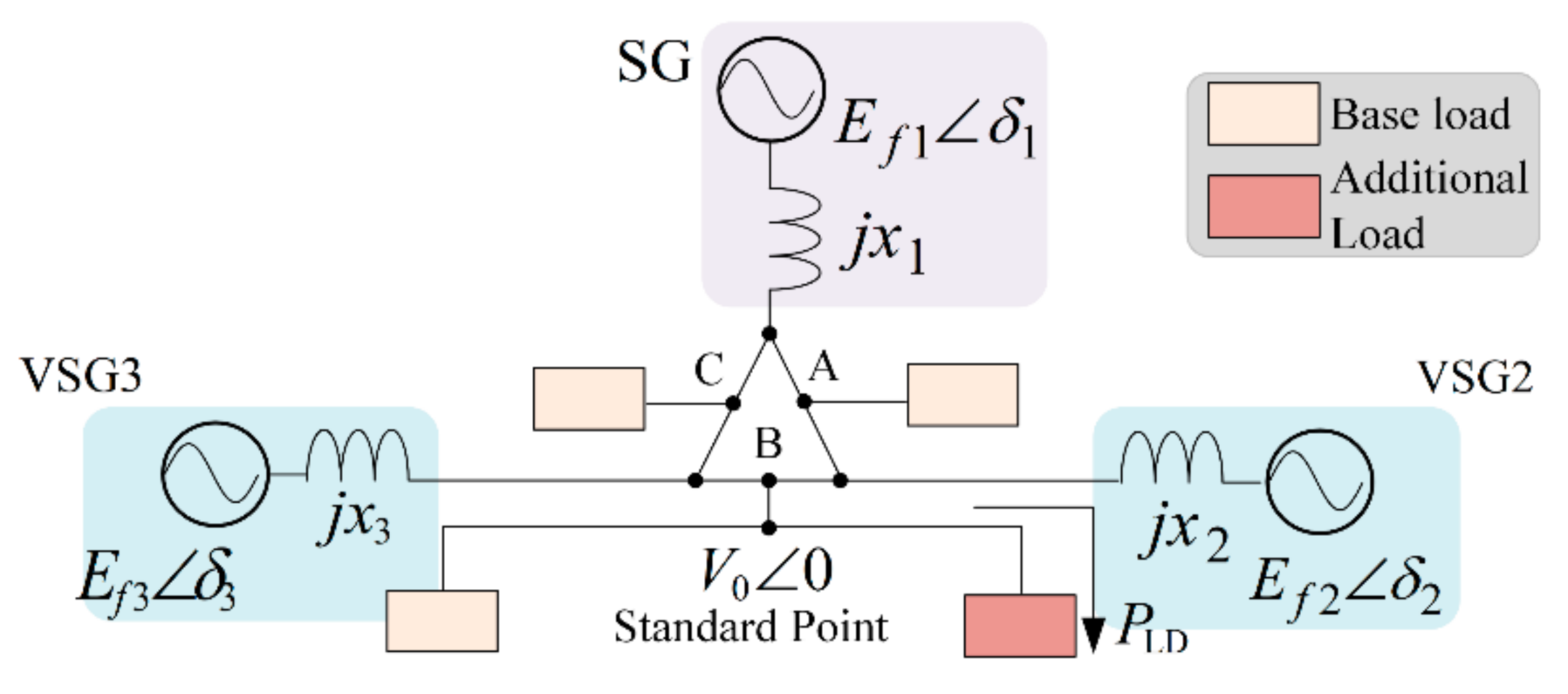
In this study, N synchronous machines are connected in a system: one primary power supply is assumed to be an SG, and (N = 1) generators are assumed to be distributed power sources. The IEEE 9 bus model (N = 3 machine systems) is adopted, and two inverters equipped with the same VSG control are connected. The two VSG inverters are contracted, and a test in which the total capacity, inertia, reactance, and other variables are converted based on the combination of the two inverters being approximately equal to the SG is used as the standard test. In other tests, the VSG control parameter was increased or decreased for comparative purposes. In this study, we do not focus on the DC side of the inverter: we assume a constant DC power supply, and the capacity of DC side is not limited.

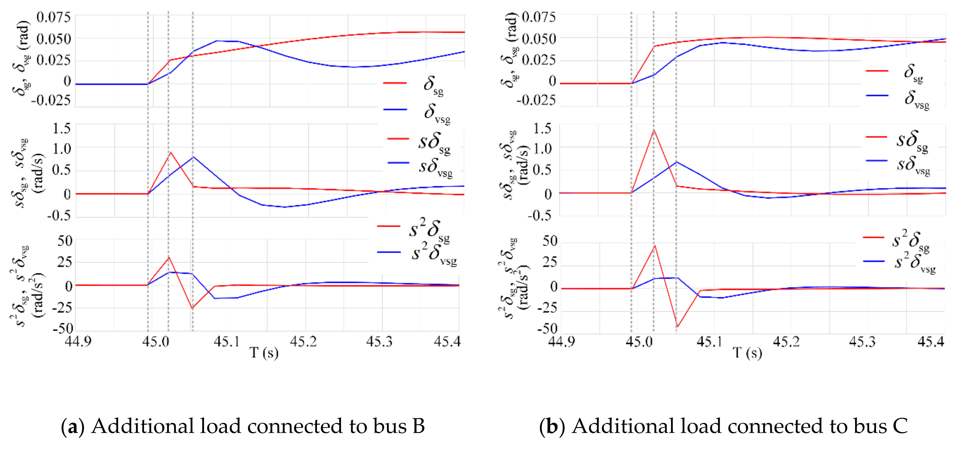
Figure 3 shows a connection diagram for the system. The base loads are evenly connected to the three buses A, B, and C between pairs of power supplies. For the purpose of running the simulation smoothly, the total base-load capacity is supplied from the SG, and an additional load is stepped onto bus B between the two VSG inverters after the power supply for the base loads has settled. The frequency deviation for the base load is compensated by the SG torque command value, and the phase difference angle after settling is subtracted as an initial offset value. The voltage deviation is considered to be small, and the terminal voltage of each power supply where the additional load is connected is assumed to be equal to the standard voltage at $V_0\angle 0$.

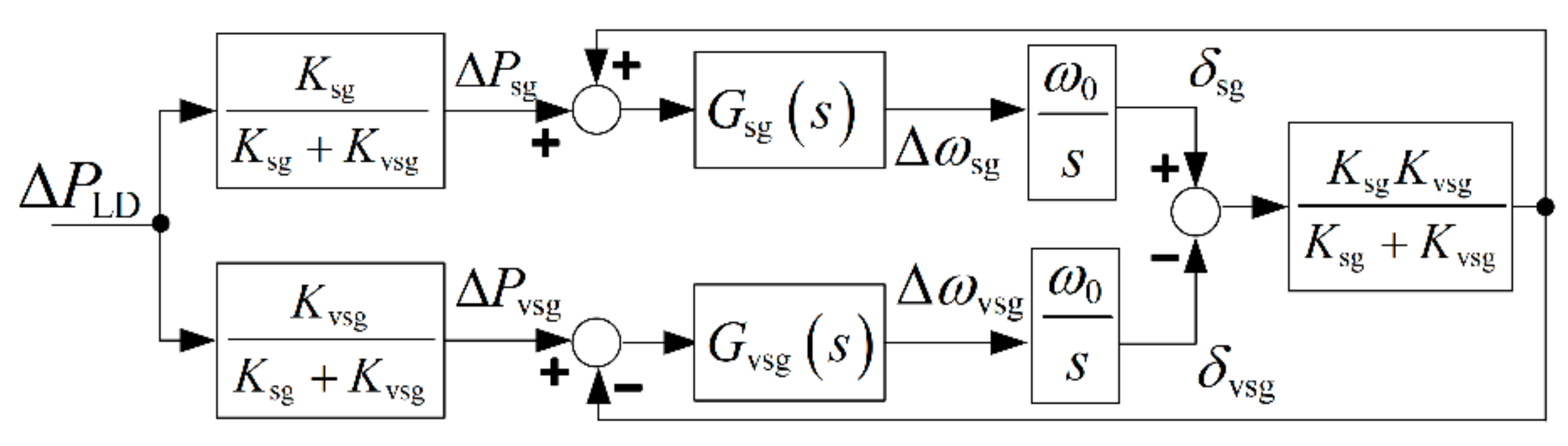
Figure 4 presents a power–frequency control block diagram of two synchronous machines [31]. $G_{\mathrm{sg}}(s)$ and $G_{\mathrm{vsg}}(s)$ indicate the same responses as those in Figure 1 and Figure 2, and the governor models $H_{\mathrm{sg}}(s)$ and $H_{\mathrm{vsg}}(s)$ are considered along with the inertial and dumping characteristics. Herein, the subscripts “sg” and “vsg” represent the SG and the contracted devices of VSG2 and VSG3 in Figure 3, respectively, and subscript “0” represents the initial value. The block diagram in Figure 4 shows the equation of motion (the swing equation) of the difference in rotor phase angles (${\delta }_{\mathrm{sg}}$ and ${\delta }_{\mathrm{vsg}}$) in the two-machine system. $\Delta P_{\mathrm{sg}}$ and $\Delta P_{\mathrm{vsg}}$ denote the difference when the load is added between the mechanical input and the electrical output of the generator for the SG and VSG, respectively. The mechanical input from the prime mover is received by the rotor of each generator. 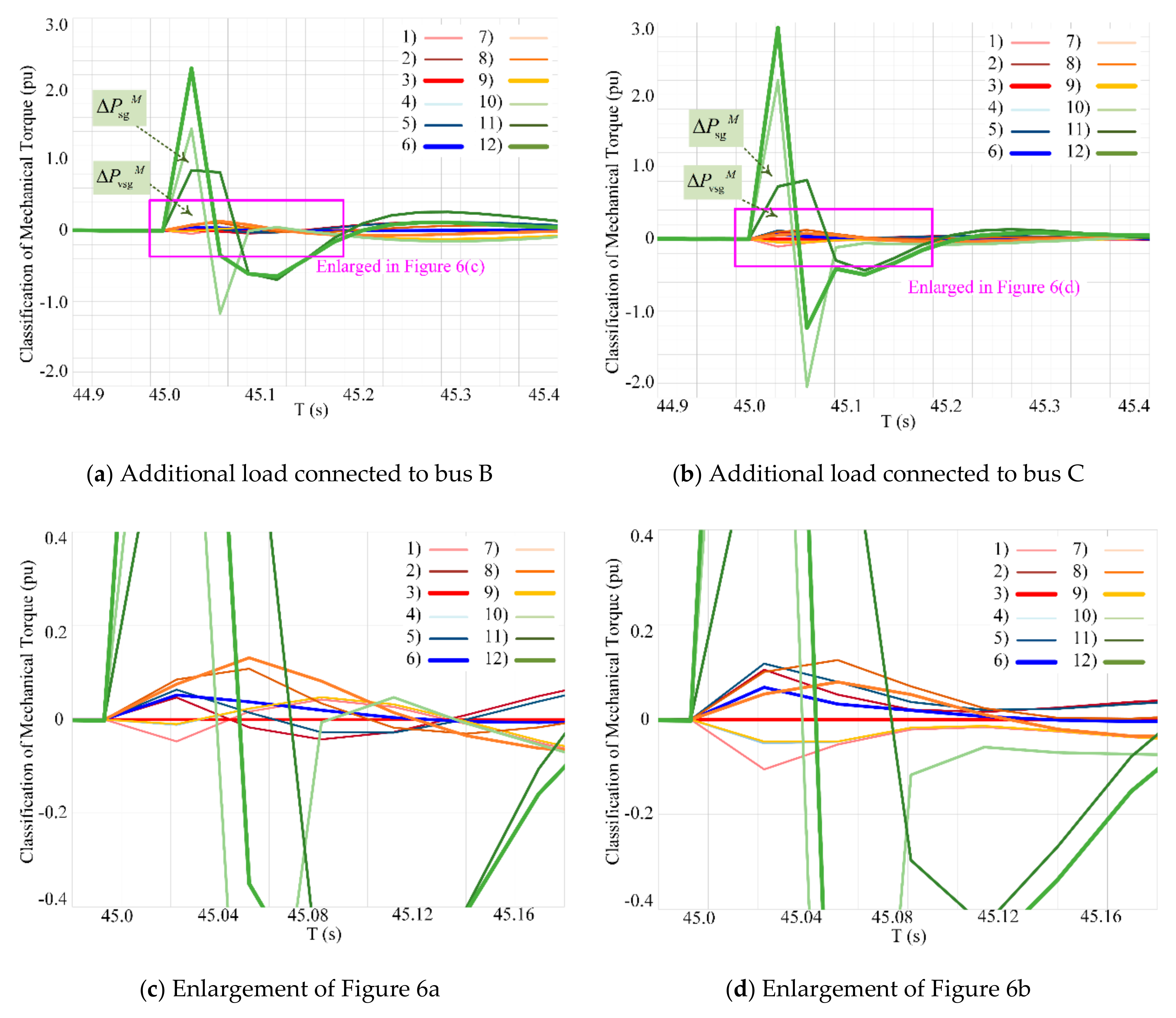Equation (1) and each order term of the phase difference angles ${\delta }_{\mathrm{sg}}$ and ${\delta }_{\mathrm{vsg}}$ in Figure 4 represent the torque types, which can be decomposed as shown in Equation (3). Hereafter, the subscript “n” refers to either “sg” or “vsg”:

$$\left\{\begin{array}{l}\Delta P_{\mathrm{n}}{}^M=\frac{M_{\mathrm{n}}}{{\omega }_0}{s}^2{\delta }_{\mathrm{n}}\\ \Delta P_{\mathrm{n}}{}^D=\frac{D_{\mathrm{n}}}{{\omega }_0}s{\delta }_{\mathrm{n}}\\ \Delta P_{\mathrm{n}}{}^R=\frac{1/R_{\mathrm{n}}}{{\omega }_0(1+s{T}_{\mathrm{n}})}s{\delta }_{\mathrm{n}}\\ \Delta P^K=K({\delta }_{\mathrm{sg}}-\hspace{0.17em}{\delta }_{\mathrm{vsg}})\end{array}\right.,$$

(3)

where $K=K_{\mathrm{sg}}{K}_{\mathrm{vsg}}/(K_{\mathrm{sg}}+K_{\mathrm{vsg}})$ is the synchronization force generated when the two synchronous machines are operated in parallel, which can be represented by the feedback of an opposite force determined by multiplying the difference in the phase angle between the two machines ${\delta }_{\mathrm{sg}}-{\delta }_{\mathrm{vsg}}$ by $K$. $K_{\mathrm{sg}}$ and $K_{\mathrm{vsg}}$ can be expressed by Equation (4):

$$\left\{\begin{array}{l}{K}_{\mathrm{sg}}=\frac{E{f}_{sg}{}_0{V}_0}{x_{\mathrm{sg}}}\cos {\delta }_{\mathrm{sg}}{}_0\\ K_{\mathrm{vsg}}=\frac{E{f}_{vsg}{}_0{V}_0}{x_{\mathrm{vsg}}}\cos {\delta }_{\mathrm{vsg}}{}_0\end{array}\right..$$

(4)

These expressions can be simplified to $K_{\mathrm{sg}}=1/x_{\mathrm{sg}}$ and $K_{\mathrm{vsg}}=1/x_{\mathrm{vsg}}$ by assuming that the voltage deviations are small and that they offset the initial value of the phase difference angle. In that case, $x_{\mathrm{sg}}$ and $x_{\mathrm{vsg}}$ correspond to the transient reactance of the SG ($x_d\text{'}$) and the virtual inductance of the VSG control ($x$), respectively.

$\Delta P_{sg}$ and $\Delta P_{vsg}$ can be expressed as the sum of each type of torque, as shown in Equation (5); they are input by proportionally distributing the variable load power $\Delta P_{\mathrm{LD}}$ that corresponds to $K_{\mathrm{sg}}$ and $K_{\mathrm{vsg}}$, as shown in Equation (6):

$$\left\{\begin{array}{l}\Delta P_{\mathrm{sg}}=\Delta P_{\mathrm{sg}}{}^M+\Delta P_{\mathrm{sg}}{}^D+\Delta P_{\mathrm{sg}}{}^R-\Delta P^K\\ \Delta P_{\mathrm{vsg}}=\Delta P_{\mathrm{vsg}}{}^M+\Delta P_{\mathrm{vsg}}{}^D+\Delta P_{\mathrm{vsg}}{}^R+\Delta P^K\end{array}\right.,$$

(5)

$$\Delta P_{\mathrm{LD}}=\frac{K_{\mathrm{sg}}+K_{\mathrm{vsg}}}{K_{\mathrm{sg}}}\Delta P_{\mathrm{sg}}+\frac{K_{\mathrm{sg}}+K_{\mathrm{vsg}}}{K_{\mathrm{vsg}}}\Delta P_{\mathrm{vsg}}.$$

(6)

The first-order differential of the phase difference angle of the rotor is the angular velocity of the system (at the reference voltage), and the second-order differential is the inertial torque, which has a relatively large value. Therefore, in the following sections, the mechanism responsible for the frequency deviations of the system during load fluctuation is analyzed using the differential equations of the phase difference angles (Equations (3)–(6)).

3. Results of Transient Response Analysis

3.1. Analysis of Mechanical Torque

Numerical simulations were conducted with MATLAB/Simulink based on the connection diagram in Figure 3, and the resulting phase difference angles ${\delta }_{\mathrm{sg}}$ and ${\delta }_{\mathrm{vsg}}$ were used to calculate Equations (3)–(6), described in Section 2.3. However, because differentiation of the simulation log data would greatly amplify the errors in the simulation calculation, the data was decimated for approximately 30 ms. Even though there were few samples due to the limitations of the simulation algorithms and the lack of computer processing power, the trend of data deviations was not suppressed.

Table 1. Machine constants and control variables.

Machine	Test Case	Reactance	Dumping Coefficient	Unit Inertia Constant	Droop Constant	Time Constant of Governor
		${\mathit{X}}_{\mathbf{n}}\left(\mathbf{pu}\right)$	${\mathit{D}}_{\mathbf{n}} (\mathbf{pu}/\mathbf{pu})$	${\mathit{M}}_{\mathbf{n}} \left(\mathbf{s}\right)$	${\mathit{R}}_{\mathbf{n}} (\%)$	${\mathit{T}}_{\mathbf{n}} \left(\mathbf{s}\right)$
SG	#1–#11	0.296	6.250	7.50	2.5	0.25
	#12	0.296	6.250	7.50	2.5	0.05
	#13					1.00
VSG (Total of two machines)	#1, #12, #13	0.296	6.250	7.50	2.5	0.25
	#2	0.296	3.125	3.75	2.5	0.25
	#3		12.50	15.0
	#4		2.083	2.50
	#5		18.75	22.5
	#6	0.200	6.250	7.50	2.5	0.25
	#7	0.400
	#8	0.592
	#9	0.800
	#10	0.296	6.250	7.50	0.25	0.25
	#11				15

lists the main machine constants and control variables of the SG and VSG for the 13 tests that were conducted. In the standard test (#1), the total capacity, inertia, reactance, and droop coefficient of the VSG are approximately the same as for the SG. All analyses were conducted using unit capacitance. The rated capacitance of the SG and VSG on the simulation circuit in standard test #1 was set to 200 MVA as 1 pu, and a line impedance of approximately 300 km was added to buses A, B, and C. The governor time constant of the VSG ($T_{\mathrm{vsg}}$) was fixed at 0 s according to the Kawasaki topology, and the droop coefficient of the SG ($R_{\mathrm{sg}}$) was fixed at 2.5%. The relationship between the dumping coefficient $D_{\mathrm{n}}$, unit inertia constant $M_n$, and damping time constant $T_d{}_{\mathrm{n}}$ was established with the equation $T_d{}_{\mathrm{n}}=2M_{\mathrm{n}}/D_{\mathrm{n}}$. Thus, the phase difference angle ${\delta }_{\mathrm{n}}$ (or $s{\delta }_{\mathrm{n}}$) estimated in the simulations was used to read the damping time constant $T_d{}_{\mathrm{n}}$ and to calculate the dumping coefficient $D_{\mathrm{n}}$. We also conducted a test in which the unit inertia constants of VSG2 and VSG3 were set to different values: 2.50 s and 5.00 s, respectively (results not included in table). Compared with test #1, in which the inertia constants of the two VSG machines were equal, only a slight difference was observed. Therefore, all subsequent analyses were performed using the results from the test in which the inertia constants of the two VSG machines were equal.

Figure 5 shows the transient response of the internal phase difference angle between the SG and two VSGs in test #1. A load of 60 MW was added 45 s after the onset of the simulations. Figure 5a, in which an additional load was connected to bus B between the two VSGs, can be compared with Figure 5b, in which the loads connected to bus C between the SG and one VSG within a 0.5 s interval. The fluctuation in the onset time slightly before 45 s can be attributed to the necessary interpolations after the decimation of the log data. As shown in Figure 5, the phase difference angle of the SG (${\delta }_{\mathrm{sg}}$) increases relatively uniformly at any load connection position (Figure 5a,b), and positive and negative vibrations of $s{\delta }_{\mathrm{n}}$ and $s^2{\delta }_{\mathrm{n}}$ occur for approximately 200 ms after the load is added.

Figure 6 shows the classification of the mechanical torque calculated using the results shown in Figure 5 and Equations (3)–(6): the synchronization torque $\Delta P_{\mathrm{n}}{}^K$ (red); the sum of the dumping and synchronization torques ($\Delta P_{\mathrm{n}}{}^D$ and $\Delta P_{\mathrm{n}}{}^K$) (blue); the sum of the governor effect ($\Delta P_{\mathrm{n}}{}^R$) and the dumping and synchronization torques ($\Delta P_{\mathrm{n}}{}^D$ and $\Delta P_{\mathrm{n}}{}^K$) (orange); and the sum of the inertial torque ($\Delta P_{\mathrm{n}}{}^M$), governor effect ($\Delta P_{\mathrm{n}}{}^R$), and dumping and synchronization torques ($\Delta P_{\mathrm{n}}{}^D$ and $\Delta P_{\mathrm{n}}{}^K$) (green). The lighter lines are for the SG, the darker lines are for the VSG, and the thick lines indicate the total value of the SG and VSG.

The area between the red and blue lines is the dumping characteristic: because the lines are nearly overlapping, the dumping characteristic can be considered to be minimal. The area between the blue and yellow lines represents the governor effect, with governor time constants for the SG and VSG of 0.25 s and 0 s, respectively. Only the VSG governor effect $\Delta P_{\mathrm{vsg}}{}^R$ is expressed immediately after the load is added. The dumping and governor effects are minimal because $s{\delta }_{\mathrm{n}}$ is minimal relative to $s^2{\delta }_{\mathrm{n}}$, and the inertial torque acting on $s^2{\delta }_{\mathrm{n}}$ becomes predominant in the time domain.

The inertial torque $\Delta P_{\mathrm{n}}{}^M$ is represented by the area between the yellow and green lines. Both inertial torques $\Delta P_{\mathrm{sg}}{}^M$ and $\Delta P_{\mathrm{vsg}}{}^M$ oscillate between positive and negative for approximately 200 ms immediately after the load is added, and SG generates a larger inertial torque than VSG (the lighter green lines are larger than the darker green lines). The effect of the connection position of the additional load is reflected in the inertial torque, which is larger when the synchronous machine is closer to the additional load and smaller when it is farther away. This may be due to the increase and decrease in the phase difference angles ${\delta }_{\mathrm{sg}}$ and ${\delta }_{\mathrm{vsg}}$ resulting from the line impedance.

Figure 7 provides a comparison of the total mechanical torque $\Delta P_{\mathrm{LD}}$ in tests #1 through #9. The parameters for tests #10–#13 (the droop coefficient $R_{\mathrm{n}}$ and governor time constant $T_{\mathrm{n}}$) are omitted because they cause minor changes in the time range for which the transient torque response is considered. Test #1 is used as a reference (purple). The results of changing the VSG unit inertia constant $M_{\mathrm{vsg}}$ are shown in Figure 7a (red), and the results of changing the virtual impedance $X_{\mathrm{vsg}}$ are shown in Figure 7b (blue). The dumping coefficient $D_{\mathrm{vsg}}$ depends on the unit inertia constant $M_{\mathrm{vsg}}$; this is not discussed here because the ratio of dumping effects is small, as mentioned above. The virtual impedance $X_{\mathrm{n}}$, which is composed of the reactance and half the value of its resistance, was also changed. In Table 1, $X_{\mathrm{n}}$ refers to the transient reactance of the SG $x_d\text{'}$ or virtual inductance $x$ of the VSG, and the resistance is not listed.

As shown in Figure 5 and Figure 6, the inertial torque becomes predominant at approximately 200 ms, after load fluctuations. Thus, Figure 7a,b indicate that changes in the VSG unit inertia constant $M_{\mathrm{vsg}}$ (Figure 7a) have a greater impact on the mechanical torque than do changes in the virtual impedance $X_{\mathrm{vsg}}$ (Figure 7b). An increase in the VSG unit inertia constant $M_{\mathrm{vsg}}$ increases the total deviations of the mechanical torque $\Delta P_{\mathrm{LD}}$ (Figure 7a). Increasing the VSG virtual impedance value has a similar effect (Figure 7b). According to Equation (3), $X_{\mathrm{vsg}}$ affects the coefficient that determines the synchronization force $\Delta P^K$, but the contribution of $\Delta P^K$ to the total torque is minimal, as indicated by the red line in Figure 6. That is, in the change in $X_{\mathrm{vsg}}$, it is presumed that the change of the output distribution in Equation (6) has a dominant effect on the mechanical torque $\Delta P_{\mathrm{LD}}$ rather than the change of the synchronization force $\Delta P^K$.

The results of test #6 in Figure 7b also indicate that the mechanical torque begins to oscillate. In test #6, the VSG virtual impedance $X_{\mathrm{vsg}}$ is set to its smallest value. Whether the oscillation can be attributed to the control stability limit of the Kawasaki VSG or to the resonance of impedance between the SG and VSG is debatable; this can constitute a topic for a future study.

3.2. Analysis of System Frequency

Figure 8 shows a comparison of the frequency deviations at the terminal voltages of each power supply. Although the droop and governor effects appear at the steady-state frequency, transitions from the transient period cannot be ignored. Hence, subsequent frequency evaluations were conducted to compare all the tests (#1 to #13). The evaluation period was set to 1.0 s after the load-power fluctuation; this exceeds the torque evaluation period of 0.5 s. Figure 8a shows the results for the cases in which the VSG unit inertia constant $M_{\mathrm{vsg}}$ was changed (red); Figure 8b shows the results when the virtual impedance $X_{\mathrm{vsg}}$ was changed (blue); Figure 8c shows the results when the droop coefficient $R_{\mathrm{vsg}}$ was changed (green); and Figure 8d shows the results when the SG governor time constant $T_{\mathrm{sg}}$ was changed (orange). The upper and lower graphs in Figure 8a–d show the frequency deviations $\Delta F_{\mathrm{sg}}$ and $\Delta F_{\mathrm{vsg}}$ [Hz] calculated from the terminal voltages of the SG and VSG, respectively. The positive and negative signs are inverted in Figure 8 to match the plots of mechanical torque in Figure 5, Figure 6 and Figure 7 in the previous section.

Figure 8a shows that for approximately 50 ms after the load is added, there is no difference in test conditions #1–#5 for the frequencies of both the SG and VSG. During the subsequent 100 ms, the frequency deviations of the SG and VSG can be recovered by setting a large unit inertia constant $M_{\mathrm{vsg}}$. This finding is consistent with Figure 7a. Meanwhile, as shown in Figure 8b, there is a minor difference in the frequencies of the test cases immediately and approximately 150 ms after the load is added. Although this result does not appear in the order of magnitude $X_{\mathrm{vsg}}$, the frequency deviations of the SG and VSG can be recovered by setting a larger VSG virtual impedance $X_{\mathrm{vsg}}$, which is also consistent with the results in Figure 7b. These results show that the impedance has a profound influence on the frequency deviation at the output terminals of the SG and VSG immediately after the load fluctuation and at intervals of 50 ms in subsequent periods. It may be that difference in the frequencies of the test cases are not observed 50 ms after the load is added (particularly for Figure 8a), due to the influence of the actual impedance (which affected all test cases equally) rather than that of the inertial torque shown in Figure 7a.

In test case #10 in Figure 8c, the VSG supplies most of the load power in the steady state, and the frequency deviations during this period are smallest for both the SG and VSG. Meanwhile, the frequency deviations are large for both the SG and VSG when the proportion of the load power in the steady state is large in the SG, as in test case #11. The differences, in the effects of changing the VSG droop coefficient (Figure 8c) and SG governor time constant (Figure 8d), are not confirmed immediately and 100 ms after the load is added and gradually increase during the transition period. Finally, they can be clearly confirmed in their steady states. These tendencies are similar to Figure 8a.

The frequency deviations in both generators diminish as the SG load sharing decreases (Figure 8c) and the SG governor delay time decreases (Figure 8d). This is because the swing (slack) bus is set such that the imbalance between the generated power and the load power of the entire system is compensated by the SG. It can be said that the mechanical torque lost from the swing node in the transient period after the load-power fluctuation determines the frequency deviation in the entire system. Thus, compensating for the lost mechanical torque at an early stage leads to an improvement in the frequency deviation.

We therefore introduce the concept of the frequency deviation of the center of inertia $\Delta F_c$ [Hz] [42], which can be considered to be the frequency deviation that exists as a common component of the entire power system. The frequency deviation of the center of the inertia $\Delta F_c$ [Hz] can be obtained from Equation (7) [42]; the results are shown in Figure 9. Herein, $\Delta F_{\mathrm{sg}}$ and $\Delta F_{\mathrm{vsg}}$ [Hz], $W_{\mathrm{sg}}$ and $W_{\mathrm{vsg}}$ [VA], and $M_{\mathrm{sg}}$ and $M_{\mathrm{vsg}}$ [s] are the frequency deviations by the terminal voltages, the rated capacities, and the unit inertia constants of SG and VSG, respectively, $F_0$ [Hz] is the nominal frequency:

$$\left\{\begin{array}{l}{\stackrel{\sim }{M}}_{\mathrm{vsg}}=\frac{M_{\mathrm{vsg}}{W}_{\mathrm{vsg}}}{F_0},\hspace{0.17em}\hspace{0.17em}{\stackrel{\sim }{M}}_{\mathrm{sg}}=\frac{M_{\mathrm{sg}}{W}_{\mathrm{sg}}}{F_0}\\ \Delta F_c=\frac{{\stackrel{\sim }{M}}_{\mathrm{vsg}}\Delta F_{\mathrm{vsg}}+{\stackrel{\sim }{M}}_{\mathrm{sg}}\Delta F_{\mathrm{sg}}}{{\stackrel{\sim }{M}}_{\mathrm{vsg}}+{\stackrel{\sim }{M}}_{\mathrm{sg}}}\end{array}\right..$$

(7)

As in Figure 8, the results associated with changes in the VSG unit inertia constant $M_{\mathrm{vsg}}$ are shown in Figure 9a (red); those associated with changes in the virtual impedance $X_{\mathrm{vsg}}$ are shown in Figure 9b (blue); those associated with changes in the droop coefficient $R_{\mathrm{vsg}}$ are shown in Figure 9c (green); and those associated with changes in the SG governor time constant $T_{\mathrm{sg}}$ are shown in Figure 9d (orange). The positive and negative signs are inverted, as in Figure 7 and Figure 8. Figure 9 can be regarded as depicting the center of gravity of the frequency deviations of both the SG and SVG in Figure 8. This can be understood based on the fact that $\Delta F_c$ [Hz] is calculated from the rotor kinetic energy by considering the size of each power source. As seen in Figure 8, because the frequency measured by the terminal voltage varies with respect to the capacity and parameters of each power supply, it is difficult to obtain a unique index of the frequency of the entire system. With regard to the aforementioned factors, we propose utilization of the concept of the center of inertia frequency and use it as a representative of the frequency of the entire system.

In the following section, the indices of the deviation and the rate of change of the center of inertia frequency are measured for the purpose of stabilizing the frequency of the entire system. The correlations between the indices and the generator parameters are also provided.

4. Discussion of the Indexing of System Frequency Deviations

4.1. Indices of the System Frequency Deviation Based on the Parameters and Time Range

We calculated the correlation between the generator control variables and equipment constants and the frequency deviation and rate of change of frequency. Figure 10 and Figure 11 show the frequency deviation and rate of change of frequency (RoCoF), respectively.

The 1.0 s time period after the load-power fluctuation is depicted on the X-axis, the generator parameters are on the Y-axis, and the frequency deviation or the RoCoF is on the Z-axis. The color of the graph surface represents the value on the Z-axis, with yellow indicating larger values and dark blue indicating smaller values. As discussed in the previous sections, the generator mechanical torque determines the frequency deviation of the entire system in the transient period immediately after the load-power fluctuation. Therefore, to achieve the three-dimensional (3D) graph visualizations, this 1.0 s time period is divided into intervals of increasing width: [0 s, 0.05 s], [0.05 s, 0.1 s], [0.1 s, 0.15 s], [0.15 s, 0.2 s], [0.2 s, 0.3 s], [0.3 s, 0.4 s], [0.4 s, 0.6 s], [0.6 s, 0.8 s], and [0.8 s, 1.0 s]. Figure 10 shows the maximum frequency deviation in each interval calculated from Figure 9. Similarly, in Figure 11, the RoCoF in each interval is calculated from Figure 9. The calculated maximum frequency deviation and RoCoF are approximated as those in the middle of the intervals.

Table A1. Maximum frequency deviations (Hz) ($M_{\mathrm{vsg}}$ was changed).

Period (s)	${\mathit{M}}_{\mathbf{vsg}}/{\mathit{M}}_{\mathbf{sg}}$
	0.333	0.500	1.000	2.000	3.000
[0, 0.05]	−0.058	−0.062	−0.073	−0.083	−0.089
[0.05, 0.1]	−0.096	−0.090	−0.082	−0.080	−0.084
[0.1, 0.15]	−0.138	−0.127	−0.107	−0.079	−0.064
[0.15, 0.2]	−0.176	−0.163	−0.139	−0.102	−0.080
[0.2, 0.3]	−0.225	−0.214	−0.186	−0.143	−0.114
[0.3, 0.4]	−0.246	−0.237	−0.213	−0.171	−0.140
[0.4, 0.6]	−0.247	−0.239	−0.222	−0.196	−0.171
[0.6, 0.8]	−0.219	−0.221	−0.218	−0.205	−0.192
[0.8, 1.0]	−0.188	−0.193	−0.204	−0.206	−0.202
1.0	−0.187	−0.190	−0.198	−0.205	−0.202

,

Table A2. Maximum frequency deviations (Hz) ($X_{\mathrm{vsg}}$ was changed).

Period (s)	${\mathit{X}}_{\mathbf{vsg}}/{\mathit{X}}_{\mathbf{sg}}$
	0.676	1.000	1.351	2.000	2.703
[0, 0.05]	−0.062	−0.073	−0.098	−0.086	−0.086
[0.05, 0.1]	−0.077	−0.082	−0.098	−0.087	−0.087
[0.1, 0.15]	−0.106	−0.107	−0.112	−0.106	−0.103
[0.15, 0.2]	−0.139	−0.139	−0.142	−0.131	−0.131
[0.2, 0.3]	−0.187	−0.186	−0.190	−0.183	−0.177
[0.3, 0.4]	−0.214	−0.213	−0.216	−0.210	−0.203
[0.4, 0.6]	−0.222	−0.222	−0.222	−0.219	−0.209
[0.6, 0.8]	−0.219	−0.218	−0.218	−0.216	−0.205
[0.8, 1.0]	−0.205	−0.204	−0.205	−0.203	−0.192
1.0	−0.198	−0.198	−0.201	−0.198	−0.189

,

Table A3. Maximum frequency deviations (Hz) ($R_{\mathrm{vsg}}$ was changed).

Period (s)	${\mathit{R}}_{\mathbf{vsg}}/{\mathit{R}}_{\mathbf{sg}}$
	0.1	1.0	4.0	6.0
[0, 0.05]	−0.073	−0.073	−0.073	−0.073
[0.05, 0.1]	−0.072	−0.082	−0.086	−0.085
[0.1, 0.15]	−0.063	−0.107	−0.119	−0.119
[0.15, 0.2]	−0.067	−0.139	−0.164	−0.166
[0.2, 0.3]	−0.069	−0.186	−0.243	−0.251
[0.3, 0.4]	−0.067	−0.213	−0.305	−0.319
[0.4, 0.6]	−0.051	−0.222	−0.357	−0.381
[0.6, 0.8]	−0.021	−0.218	−0.360	−0.387
[0.8, 1.0]	−0.045	−0.204	−0.356	−0.385
1.0	−0.045	−0.198	−0.347	−0.377

and

Table A4. Maximum frequency deviations (Hz) ($T_{\mathrm{sg}}$ was changed).

Period (s)	${\mathit{T}}_{\mathbf{sg}} \left(\mathbf{s}\right)$
	0.05	0.10	0.25	0.50	1.00
[0, 0.05]	−0.072	−0.072	−0.073	−0.072	−0.073
[0.05, 0.1]	−0.079	−0.080	−0.082	−0.082	−0.082
[0.1, 0.15]	−0.099	−0.103	−0.107	−0.108	−0.109
[0.15, 0.2]	−0.126	−0.131	−0.139	−0.141	−0.144
[0.2, 0.3]	−0.163	−0.171	−0.186	−0.195	−0.202
[0.3, 0.4]	−0.182	−0.191	−0.213	−0.231	−0.244
[0.4, 0.6]	−0.190	−0.197	−0.222	−0.249	−0.278
[0.6, 0.8]	−0.190	−0.196	−0.218	−0.249	−0.278
[0.8, 1.0]	−0.191	−0.192	−0.204	−0.232	−0.270
1.0	−0.191	−0.192	−0.198	−0.216	−0.254

in Appendix A list the maximum frequency deviations of the intervals for all parameters used in the calculations for Figure 10 and Figure 11, and

Table A5. Rate of change of frequency (RoCoF) (Hz/s) ($M_{\mathrm{vsg}}$ was changed).

Period (s)	${\mathit{M}}_{\mathbf{vsg}}/{\mathit{M}}_{\mathbf{sg}}$
	0.333	0.500	1.000	2.000	3.000
[0, 0.05]	−1.128	−1.245	−1.409	−1.586	−1.680
[0.05, 0.1]	−0.743	−0.569	−0.184	0.233	0.448
[0.1, 0.15]	−0.821	−0.742	−0.509	−0.205	−0.033
[0.15, 0.2]	−0.728	−0.714	−0.620	−0.448	−0.333
[0.2, 0.3]	−0.503	−0.501	−0.492	−0.426	−0.358
[0.3, 0.4]	−0.195	−0.214	−0.255	−0.272	−0.245
[0.4, 0.6]	0.138	0.082	−0.022	−0.124	−0.152
[0.6, 0.8]	0.157	0.142	0.073	−0.041	−0.107
[0.8, 1.0]	0.006	0.015	0.032	−0.002	−0.047

,

Table A6. RoCoF (Hz/s) ($X_{\mathrm{vsg}}$ was changed).

Period (s)	${\mathit{X}}_{\mathbf{vsg}}/{\mathit{X}}_{\mathbf{sg}}$
	0.676	1.000	1.351	2.000	2.703
[0, 0.05]	−1.010	−1.409	−1.898	−1.606	−1.678
[0.05, 0.1]	−0.310	−0.184	0.054	−0.020	0.009
[0.1, 0.15]	−0.583	−0.509	−0.368	−0.382	−0.337
[0.15, 0.2]	−0.642	−0.620	−0.581	−0.575	−0.557
[0.2, 0.3]	−0.491	−0.492	−0.490	−0.502	−0.479
[0.3, 0.4]	−0.252	−0.255	−0.244	−0.258	−0.240
[0.4, 0.6]	−0.025	−0.022	−0.010	−0.025	−0.010
[0.6, 0.8]	0.075	0.073	0.068	0.063	0.069
[0.8, 1.0]	0.035	0.032	0.023	0.027	0.016

,

Table A7. RoCoF (Hz/s) ($R_{\mathrm{vsg}}$ was changed).

Period (s)	${\mathit{R}}_{\mathbf{vsg}}/{\mathit{R}}_{\mathbf{sg}}$
	0.1	1.0	4.0	6.0
[0, 0.05]	−1.406	−1.409	−1.419	−1.162
[0.05, 0.1]	0.185	−0.184	−0.253	−0.254
[0.1, 0.15]	0.016	−0.509	−0.681	−0.694
[0.15, 0.2]	−0.087	−0.620	−0.882	−0.916
[0.2, 0.3]	−0.006	−0.492	−0.822	−0.877
[0.3, 0.4]	0.158	−0.255	−0.600	−0.657
[0.4, 0.6]	0.182	−0.022	−0.253	−0.305
[0.6, 0.8]	−0.030	0.073	0.003	−0.018
[0.8, 1.0]	−0.124	0.032	0.050	0.041

and

Table A8. RoCoF ($T_{\mathrm{sg}}$ was changed).

Period (s)	${\mathit{T}}_{\mathbf{sg}} \left(\mathbf{s}\right)$
	0.05	0.10	0.25	0.50	1.00
[0, 0.05]	−1.111	−1.140	−1.409	−1.145	−1.123
[0.05, 0.1]	−0.131	−0.155	−0.184	−0.187	−0.192
[0.1, 0.15]	−0.421	−0.458	−0.509	−0.528	−0.544
[0.15, 0.2]	−0.506	−0.547	−0.620	−0.657	−0.682
[0.2, 0.3]	−0.379	−0.411	−0.492	−0.558	−0.601
[0.3, 0.4]	−0.181	−0.189	−0.255	−0.340	−0.405
[0.4, 0.6]	−0.040	−0.023	−0.022	−0.083	−0.162
[0.6, 0.8]	0.000	0.018	0.073	0.085	0.039
[0.8, 1.0]	−0.003	0.002	0.032	0.077	0.081

in Appendix A list the RoCoFs of the intervals.

In Figure 10 and Figure 11, (a) shows the result of changing the VSG unit inertia constants $M_{\mathrm{vsg}}$, (b) shows the result of changing the virtual impedance $X_{\mathrm{vsg}}$, (c) shows the result of changing the droop coefficients $R_{\mathrm{vsg}}$, and (d) shows the result of changing the SG governor time constants $T_{\mathrm{sg}}$. Figure 9 shows the results of changing the parameters centered on the standard test (#1, in which the two machines have almost the same capability). Therefore, in Figure 10 and Figure 11, the VSG to SG ratio of each parameter is displayed on the Y-axis. However, because the VSG governor time constant of the Kawasaki topology is zero, the SG governor time constant $T_{\mathrm{sg}}$ is displayed on the Y-axis in Figure 10d and Figure 11d.

Both the time response of the frequency deviations and their response to changes in the main parameters can be understood simultaneously in Figure 10 and Figure 11. It can be seen from Figure 10a and Figure 11a that the inertia constant ratio and the reactance ratio strongly affect both the frequency deviation and RoCoF in this time domain. For a small inertial constant ratio, a small frequency recovery is observed immediately after the load power fluctuates, and the absolute value of RoCoF is large. However, after the frequency nadir, the recovery effect is large and the absolute value of RoCoF is small compared to the case where the inertial constant ratio is large. The opposite tendency of the reactance ratio can be observed in Figure 10b and Figure 11b. After the load power fluctuation, the smaller the reactance ratio, the smaller the frequency fluctuation and the larger the absolute value of RoCoF. However, this difference disappears over time. It is worth noting that both the inertia constant and the impedance ratios show tendencies of mountains and valleys when the ratio value is between 1 and 1.5, especially in the period immediately after the load power fluctuation. Alternatively, Figure 10c and Figure 11c show that when the droop ratio is small, the frequency deviation reduces, and the RoCoF fluctuation increases. From Figure 10d and Figure 11d, it can be inferred that the smaller the governor time constant of the SG, the smaller the frequency deviation. However, there is no significant difference in the RoCoF.

Because both the frequency deviation and the RoCoF are approximated by the values at the midpoint time of each interval, the results do not exactly match the actual measured values. The accuracy might be improved by lengthening the time period and/or by increasing the number of intervals. We plan to re-test with an increased accuracy in the future.

4.2. Indices of the System Frequency Deviation Based on the Frequency Characteristics

The frequency deviation index of each parameter in the time domain, calculated in the previous section, is examined from another angle in this section. The frequency characteristic from the load power fluctuation to the frequency fluctuation measured by the terminal voltage of each generator (${\overline{G}}_{\mathrm{vsg}}(s)$ and ${\overline{G}}_{\mathrm{sg}}(s)$) can be obtained from Equation (8) [30,31]. Here, as in Figure 1, $G_{\mathrm{vsg}}(s)=-1/(s{M}_{\mathrm{vsg}}+1/R_{\mathrm{vsg}})$ and $G_{\mathrm{sg}}(s)=-(s{T}_{\mathrm{sg}}+1)/(s^2{M}_{\mathrm{sg}}{T}_{\mathrm{sg}}+s{M}_{\mathrm{sg}}+1/R_{\mathrm{sg}})$ are stand-alone responses of the VSG and SG, respectively, and as explained above, Equation (4) can be simplified to $K_{\mathrm{vsg}}=1/X_{\mathrm{vsg}}$ and $K_{\mathrm{sg}}=1/X_{\mathrm{sg}}$. ${\omega }_0$ is the rated angular frequency:

$$\left\{\begin{array}{l}\frac{\Delta {\omega }_{\mathrm{vsg}}}{\Delta P}={\overline{G}}_{\mathrm{vsg}}(s)=\frac{G_{\mathrm{vsg}}(s)}{1+\left(\frac{{\omega }_0}{s}{G}_{\mathrm{vsg}}(s)-\frac{1}{K_{\mathrm{vsg}}}\right)/\left(\frac{{\omega }_0}{s}{G}_{\mathrm{sg}}(s)-\frac{1}{K_{\mathrm{sg}}}\right)}\\ \frac{\Delta {\omega }_{\mathrm{sg}}}{\Delta P}={\overline{G}}_{\mathrm{sg}}(s)=\frac{G_{\mathrm{sg}}(s)}{1+\left(\frac{{\omega }_0}{s}{G}_{\mathrm{sg}}(s)-\frac{1}{K_{\mathrm{sg}}}\right)/\left(\frac{{\omega }_0}{s}{G}_{\mathrm{vsg}}(s)-\frac{1}{K_{\mathrm{vsg}}}\right)}\end{array}\right..$$

(8)

To achieve an index for controlling the entire system, we introduce the center of inertial frequency in place of the frequencies by terminal voltages. The frequency characteristic of the center of inertial frequency can be derived from Equations (7) and (8); it is expressed in Equation (9):

$$\begin{array}{ll}\frac{\Delta {\omega }_c}{\Delta P}& =\frac{1}{\Delta P}\frac{{\stackrel{\sim }{M}}_{\mathrm{vsg}}\Delta {\omega }_{\mathrm{vsg}}+{\stackrel{\sim }{M}}_{\mathrm{sg}}\Delta {\omega }_{\mathrm{sg}}}{\stackrel{\sim }{M}+\mathrm{vsg}{\stackrel{\sim }{M}}_{\mathrm{sg}}}\\ \\ =\frac{{\stackrel{\sim }{M}}_{\mathrm{vsg}}}{\stackrel{\sim }{M}+\mathrm{vsg}{\stackrel{\sim }{M}}_{\mathrm{sg}}}\frac{\Delta {\omega }_{\mathrm{vsg}}}{\Delta P}+\frac{{\stackrel{\sim }{M}}_{\mathrm{sg}}}{\stackrel{\sim }{M}+\mathrm{vsg}{\stackrel{\sim }{M}}_{\mathrm{sg}}}\frac{\Delta {\omega }_{\mathrm{sg}}}{\Delta P}\end{array}$$

(9)

Using Equations (10)–(12), ${\overline{G}}_{\mathrm{vsg}}(s)$ and ${\overline{G}}_{\mathrm{sg}}(s)$ in Equation (8) can be rewritten as Equation (13). Here, ${\hat{G}}_{\mathrm{vsg}}(s)$ and ${\hat{G}}_{\mathrm{sg}}(s)$ can be considered as the transfer functions of the frequency deviations from the load power fluctuation when the VSG and SG are connecting to an infinite bus. It is clear that ${\hat{G}}_{\mathrm{vsg}}(s)$ and ${\hat{G}}_{\mathrm{sg}}(s)$ are the key factors that determine the characteristics of ${\overline{G}}_{\mathrm{vsg}}(s)$ and ${\overline{G}}_{\mathrm{sg}}(s)$:

$$\left\{\begin{array}{l}{\hat{G}}_{\mathrm{vsg}}(s)=\frac{{\omega }_0}{s}{G}_{\mathrm{vsg}}(s)-\frac{1}{K_{\mathrm{vsg}}}\\ {\hat{G}}_{\mathrm{sg}}(s)=\frac{{\omega }_0}{s}{G}_{\mathrm{sg}}(s)-\frac{1}{K_{\mathrm{sg}}}\end{array}\right.,$$

(10)

$$\left\{\begin{array}{l}{\stackrel{⌢}{G}}_{\mathrm{vsg}}(s)=\frac{\frac{{\omega }_0}{s}{G}_{\mathrm{sg}}(s)-\frac{1}{K_{\mathrm{sg}}}}{\frac{{\omega }_0}{s}{G}_{\mathrm{vsg}}(s)-\frac{1}{K_{\mathrm{vsg}}}}=\frac{{\hat{G}}_{\mathrm{sg}}(s)}{{\hat{G}}_{\mathrm{vsg}}(s)}\\ {\stackrel{⌢}{G}}_{\mathrm{sg}}(s)=\frac{\frac{{\omega }_0}{s}{G}_{\mathrm{vsg}}(s)-\frac{1}{K_{\mathrm{vsg}}}}{\frac{{\omega }_0}{s}{G}_{\mathrm{sg}}(s)-\frac{1}{K_{\mathrm{sg}}}}=\frac{{\hat{G}}_{\mathrm{vsg}}(s)}{{\hat{G}}_{\mathrm{sg}}(s)}\end{array}\right.,$$

(11)

$$\left\{\begin{array}{ll}{\tilde{G}}_{\mathrm{vsg}}(s)& =\frac{1}{1+\left(\frac{{\omega }_0}{s}{G}_{\mathrm{sg}}(s)-\frac{1}{K_{\mathrm{sg}}}\right)/\left(\frac{{\omega }_0}{s}{G}_{\mathrm{vsg}}(s)-\frac{1}{K_{\mathrm{vsg}}}\right)}=\frac{1}{1+{\stackrel{⌢}{G}}_{\mathrm{vsg}}(s)}=\frac{{\hat{G}}_{\mathrm{vsg}}(s)}{{\hat{G}}_{\mathrm{sg}}(s)+{\hat{G}}_{\mathrm{vsg}}(s)}\\ {\tilde{G}}_{\mathrm{sg}}(s)& =\frac{1}{1+\left(\frac{{\omega }_0}{s}{G}_{\mathrm{vsg}}(s)-\frac{1}{K_{\mathrm{vsg}}}\right)/\left(\frac{{\omega }_0}{s}{G}_{\mathrm{sg}}(s)-\frac{1}{K_{\mathrm{sg}}}\right)}=\frac{1}{1+{\stackrel{⌢}{G}}_{\mathrm{sg}}(s)}=\frac{{\hat{G}}_{\mathrm{sg}}(s)}{{\hat{G}}_{\mathrm{vsg}}(s)+{\hat{G}}_{\mathrm{sg}}(s)}\end{array}\right.,$$

(12)

$$\left\{\begin{array}{l}{\overline{G}}_{\mathrm{vsg}}(s)=\frac{\Delta {\omega }_{\mathrm{vsg}}}{\Delta P}=G_{\mathrm{vsg}}(s){\tilde{G}}_{\mathrm{sg}}(s)\\ {\overline{G}}_{\mathrm{sg}}(s)=\frac{\Delta {\omega }_{\mathrm{sg}}}{\Delta P}=G_{\mathrm{sg}}(s){\tilde{G}}_{\mathrm{vsg}}(s)\end{array}\right..$$

(13)

The Bode diagram in Equation (9) is shown in Figure 12. Similar to Figure 8, Figure 9, Figure 10 and Figure 11, Figure 12a shows the results of changing the VSG unit inertia constant $M_{\mathrm{vsg}}$; Figure 12b shows the results of changing the virtual impedance $X_{\mathrm{vsg}}$; Figure 12c shows the results of changing the droop coefficient $R_{\mathrm{vsg}}$; and Figure 12d shows the results of changing the SG governor time constant $T_{\mathrm{sg}}$.

Figure 12a shows that the frequency deviation can be suppressed by setting a large unit inertia constant for the VSG, as in Figure 10a. At the same time, it is evident that its phase is delayed in the band of approximately 1.0 to 10 rad/s (0.16 to 1.6 Hz). Furthermore, although interference between the two machines is seen in the band of approximately 10 rad/s (1.6 Hz), the gain in that band is sufficiently attenuated, so this does not pose a major problem. Conversely, in test cases #2 and #4, where $(M_{\mathrm{vsg}}/M_{\mathrm{sg}})<1$, the parallel operation of two machines in the frequency band where the gain is amplified must be undertaken carefully. As evident in Figure 12b, the effect of the virtual impedance of the VSG is small. It is well known that frequency deviation can be suppressed in the low frequency band (steady state) when the droop coefficient of the VSG is extremely small and the load sharing ratio is large. However, in test case #10 in Figure 12c, the gain is greatly amplified in the frequency band of approximately 10 rad/s (1.6 Hz) where the interference of the two machines occurs. Figure 12d shows that in the low frequency band (approximately 1.0 rad/s (0.16 Hz)), setting the governor time constant of the main power supply causes the gain to be amplified and the phase to lead. Figure 13 shows the poles and zeros of $G_c(s)$, ${\stackrel{⌢}{G}}_{\mathrm{vsg}}(s)$, and ${\stackrel{⌢}{G}}_{\mathrm{sg}}(s)$. As in previous figures, Figure 13a–d respectively show the results for the cases in which the VSG unit inertia constant $M_{\mathrm{vsg}}$, the virtual impedance $X_{\mathrm{vsg}}$, the droop coefficient $R_{\mathrm{vsg}}$, and the SG governor time constant $T_{\mathrm{sg}}$ are changed. The red, blue, and green symbols denote the poles and zeros of $G_c(s)$, ${\stackrel{⌢}{G}}_{\mathrm{vsg}}(s)$, and ${\stackrel{⌢}{G}}_{\mathrm{sg}}(s)$, respectively.

The three significant types of oscillating poles of $G_c(s)$ can be confirmed, and they are highlighted by light blue, yellow, and pink arrows/circles. The arrows indicate the direction in which the parameters are increasing. In the tests in which $M_{\mathrm{vsg}}$, $X_{\mathrm{vsg}}$, and $R_{\mathrm{vsg}}$ change, $G_c(s)$ has a natural frequency band (the poles in Figure 13a–c marked by light blue arrows) that is strongly influenced by ${\stackrel{⌢}{G}}_{\mathrm{vsg}}(s)$, and conversely, in the test in which $T_{\mathrm{sg}}$ changes, it has a natural frequency band (the poles in Figure 13d marked by pink arrows) that is affected by ${\stackrel{⌢}{G}}_{\mathrm{sg}}(s)$. The poles in Figure 13a–d marked by yellow arrows/circles are related to both the VSG and SG. As shown by the arrows in this figure, when the parameters are increased, the poles approach the origin. This means that even though the oscillation frequency reduces, the oscillation tends to continue. The tendency of oscillation due to the specified parameters is difficult to judge from the transient response in Figure 9, and it is also difficult to judge the time required for damping from the Bode diagram in Figure 12. Based on the aforementioned factors, it can be inferred that the pole zero map of Figure 13 effectively shows the indexed graphs of Figure 10 and Figure 11 from another angle.

5. Conclusions

In this study, a synchronous generator was used as the main power source, and multiple grid-connected inverters equipped with VSG controls were connected to the IEEE 9 bus system. The mechanical torque characteristics of each generator were decomposed and analyzed to clarify the mechanism through which each type of torque causes system frequency deviations. The correlation between the time, each parameter (control variables and equipment constants) of the main generator and grid-connected inverters, and the frequency responses was also analyzed. The findings of this study are summarized as follows:

-

In systems that include smart inverters (e.g., VSG inverters) in addition to the conventional synchronous generator, various mechanical torques in each power source cause fluctuations in the system frequency.

-

Because the frequency at the terminal voltage of each power supply of the multi-machine system is strongly influenced by the equipment constants and control variables of the power supply, we introduced the concept of “center of inertial frequency.”

-

Both the time and frequency domains of the system frequency, which are affected, differ with respect to various mechanical torque types (damping, inertia, synchronization torques, and governor effect).

-

Frequency deviations that strongly depend on both device constants/control variables and time were indexed using 3D graphs. Furthermore, to evaluate the oscillation intensity and the damping time, the pole arrangement of the system was studied.

-

A multi-machine system can be reduced to a system with only two machines consisting of a main power supply and other power supplies. The frequency fluctuation system is determined through the ratios of the equipment constants/control variables of those two machines.

It has been previously confirmed empirically that a grid-connected inverter with the characteristics of a synchronous machine can stabilize a system as the main power source in a small-scale system or an isolated MG. However, a similar problem has recently been identified in large-scale smart grids and the magnitude of faults and their contributions in the grids were not quantified. Thus, that uncertainty has impeded the introduction of distributed power sources. In this study, therefore, a quantification index that applies the two-machine contraction model is utilized to suitably set the parameters of multiple grid-connected inverters, making it possible to predict and control their effects on large smart grids. It is expected that this knowledge will contribute to accelerating the introduction of distributed power sources originating from renewable energies, thereby reducing carbon emissions.

References

1. Rashid, K. Design, Economics, and Real-Time Optimization of a Solar/Natural Gas Hybrid Power Plant. Ph.D. Thesis, The University of Utah, Salt Lake, UT, USA, 2019. [Google Scholar]
2. Sakimoto, K.; Miura, Y.; Ise, T. Stabilization of a power system with a distributed generator by a virtual synchronous generator function. In Proceedings of the IEEE Power Electronics and ECCE Asia (ICPE & ECCE), Jeju, Korea, 29 May–2 June 2011; pp. 1498–1505. [Google Scholar]
3. Bevrani, H.; Ise, T.; Miura, Y. Virtual synchronous generators: A survey and new perspectives. Int. J. Electric. Power Energy Syst. 2014, 54, 244–254. [Google Scholar] [CrossRef]
4. Verga, M.; Lazzari, R.; Johnson, J.; Rosewater, D. SIRFN Draft Test Protocols for Advanced Battery Energy Storage System Interoperability Functions; ISGAN IEA: Berlin, Germany, 2016. [Google Scholar]
5. Rashid, K.; Safdarnejad, S.M.; Powell, K.M. Dynamic simulation, control, and performance evaluation of a synergistic solar and natural gas hybrid power plant. Energy Convers. Manag. 2019, 179, 270–285. [Google Scholar] [CrossRef]
6. Bayindir, R.; Colak, I.; Fulli, G.; Demirtas, K. Smart grid technologies and applications. Renew. Sustain. Energy Rev. 2016, 66, 499–516. [Google Scholar] [CrossRef]
7. Thomas, D.; D’Hoop, G.; Deblecker, O.; Genikomsakis, K.N.; Ioakimidis, C.S. An integrated tool for optimal energy scheduling and power quality improvement of a microgrid under multiple demand response schemes. Appl. Energy 2020, 260, 114314. [Google Scholar] [CrossRef] [Green Version]
8. Olowu, T.; Sundararajan, A.; Moghaddami, M.; Sarwat, A. Future Challenges and Mitigation Methods for High Photovoltaic Penetration: A Survey. Energies 2018, 11, 1782. [Google Scholar] [CrossRef] [Green Version]
9. Lee, H.-J.; Yoon, K.-H.; Shin, J.-W.; Kim, J.-C.; Cho, S.-M. Optimal Parameters of Volt–Var Function in Smart Inverters for Improving System Performance. Energies 2020, 13, 2294. [Google Scholar] [CrossRef]
10. Ninad, N.; Abraham, K.; Srikumar, S.; Gurunathan, P.; Turcotte, D. Grid Support Functions Impact on Residential Voltage Profile for Updated Canadian Interconnection Standard. In Proceedings of the 2019 IEEE Electrical Power and Energy Conference (EPEC), Montréal, QC, Canada, 16–18 October 2019; pp. 1–6. [Google Scholar]
11. Nelson, A.; Nagarajan, A.; Prabakar, K.; Gevorgian, V.; Lundstrom, B.; Nepal, S.; Hoke, A.; Asano, M.; Ueda, R.; Shindo, J. Hawaiian Electric Advanced Inverter Grid Support Function Laboratory Validation and Analysis; National Renewable Energy Lab. (NREL): Golden, CO, USA, 2016.
12. Elkhatib, M.E.; Du, W.; Lasseter, R.H. Evaluation of inverter-based grid frequency support using frequency-watt and grid-forming PV inverters. In Proceedings of the 2018 IEEE Power & Energy Society General Meeting (PESGM), Portland, OR, USA, 5–10 August 2018; pp. 1–5. [Google Scholar]
13. Giraldez Miner, J.I.; Emmanuel, M.; Hoke, A.F.; Suryanarayanan, S. Impacts of Voltage-Based Grid-Support Functions on Energy Production of PV Customers; National Renewable Energy Lab. (NREL): Golden, CO, USA, 2019.
14. Rylander, M.; Reno, M.J.; Quiroz, J.E.; Ding, F.; Li, H.; Broderick, R.J.; Mather, B.; Smith, J. Methods to determine recommended feeder-wide advanced inverter settings for improving distribution system performance. In Proceedings of the 2016 IEEE 43rd Photovoltaic Specialists Conference (PVSC), Portland, OR, USA, 5–10 June 2016; pp. 1393–1398. [Google Scholar]
15. Chakraborty, S.; Nelson, A.; Hoke, A. Power hardware-in-the-loop testing of multiple photovoltaic inverters' volt-var control with real-time grid model. In Proceedings of the 2016 IEEE Power & Energy Society Innovative Smart Grid Technologies Conference (ISGT), Melbourne, Australia, 28 November–1 December 2016; pp. 1–5. [Google Scholar]
16. Hernandez-Alvidrez, J.; Johnson, J. Parametric PV grid-support function characterization for simulation environments. In Proceedings of the 2017 IEEE 44th Photovoltaic Specialist Conference (PVSC), Washington, DC, USA, 25–30 June 2017; pp. 2153–2158. [Google Scholar]
17. Johnson, J.; Ablinger, R.; Bruendlinger, R.; Fox, B.; Flicker, J. Interconnection Standard Grid-Support Function Evaluations using an Automated Hardware-in-the-Loop Testbed. IEEE J. Photovolt. 2018, 8, 565–571. [Google Scholar] [CrossRef]
18. Prabakar, K.; Singh, A.; Tombari, C. IEEE 1547–2018 Based Interoperable PV Inverter with Advanced Grid-Support Functions. In Proceedings of the 2019 IEEE 46th Photovoltaic Specialists Conference (PVSC), Chicago, IL, USA, 16–21 June 2019; pp. 2072–2077. [Google Scholar]
19. Montoya, J.; Brandl, R.; Vishwanath, K.; Johnson, J.; Darbali-Zamora, R.; Summers, A.; Hashimoto, J.; Kikusato, H.; Ustun, T.S.; Ninad, N.; et al. Advanced Laboratory Testing Methods Using Real-Time Simulation and Hardware-in-the-Loop Techniques: A Survey of Smart Grid International Research Facility Network Activities. Energies 2020, 13, 3267. [Google Scholar] [CrossRef]
20. Seuss, J.; Reno, M.J.; Broderick, R.J.; Harley, R.G. Evaluation of reactive power control capabilities of residential PV in an unbalanced distribution feeder. In Proceedings of the 2014 IEEE 40th Photovoltaic Specialist Conf. (PVSC), Denver, CL, USA, 8–13 June 2014; pp. 2094–2099. [Google Scholar]
21. Smith, J.W.; Sunderman, W.; Dugan, R.; Seal, B. Smart inverter volt/var control functions for high penetration of PV on distribution systems. In Proceedings of the IEEE/PES Power Systems Conf. and Exposition, Phoenix, AZ, USA, 20–23 March 2011; pp. 1–6. [Google Scholar]
22. Hirase, Y. Guidelines for required grid-supportive functions in grid-tied inverters with distributed energy resources. IET Energy Syst. Integr. 2016, 1, 236–245. [Google Scholar] [CrossRef]
23. Hoke, A.; Nelson, A.; Miller, B.; Chakraborty, S.; Bell, F.; McCarty, M. Experimental Evaluation of Pv Inverter Anti-Islanding with Grid Support Functions in Multi-Inverter Island Scenarios; National Renewable Energy Lab. (NREL): Golden, CO, USA, 2016.
24. Hashimoto, J.; Ustun, T.S.; Otani, K. Smart inverter functionality testing for battery energy storage systems. Smart Grid Renew. Energy 2017, 8, 337–350. [Google Scholar] [CrossRef] [Green Version]
25. Seuss, J.; Reno, M.J.; Lave, M.; Broderick, R.J.; Grijalva, S. Advanced inverter controls to dispatch distributed PV systems. In Proceedings of the 2016 IEEE 43rd Photovoltaic Specialists Conference (PVSC), Portland, OR, USA, 5–10 June 2016; pp. 1387–1392. [Google Scholar]
26. Kim, Y.-S.; Kim, G.-H.; Lee, J.-D.; Cho, C. New requirements of the voltage/VAR function for smart inverter in distributed generation control. Energies 2016, 9, 929. [Google Scholar] [CrossRef] [Green Version]
27. Braslavsky, J.H.; Collins, L.D.; Ward, J.K. Voltage stability in a grid-connected inverter with automatic Volt-Watt and Volt-VAR functions. EEE Trans. Smart Grid 2019, 10, 84–94. [Google Scholar] [CrossRef]
28. Boli, L.; Xiangqian, T.; Minghang, Z.; Xiaoqing, Z.; Jun, D. Local Voltage Control Strategy Based on Remaining Capacity of PV Grid-connected Inverter. In Proceedings of the 2018 IEEE International Power Electronics and Application Conference and Exposition (PEAC), Shenzhen, China, 4–7 November 2018; pp. 1–5. [Google Scholar]
29. Kashani, M.G.; Mobarrez, M.; Bhattacharya, S. Smart Inverter Volt-Watt Control Design in High PV-Penetrated Distribution Systems. IEEE Trans. Ind. Appl. 2018, 55, 1147–1156. [Google Scholar] [CrossRef]
30. Hirase, Y.; Sugimoto, K.; Sakimoto, K.; Ise, T. Analysis of resonance in microgrids and effects of system frequency stabilization using a virtual synchronous generator. IEEE J. Emerg. Sel. Top. Power Electron. 2016, 4, 1287–1298. [Google Scholar] [CrossRef]
31. Hirase, Y.; Abe, K.; Sugimoto, K.; Sakimoto, K.; Bevrani, H.; Ise, T. A novel control approach for virtual synchronous generators to suppress frequency and voltage fluctuations in microgrids. Appl. Energy 2018, 210, 699–710. [Google Scholar] [CrossRef]
32. Alipoor, J.; Miura, Y.; Ise, T. Power system stabilization using virtual synchronous generator with alternating moment of inertia. IEEE J. Emerg. Sel. Top. Power Electron. 2015, 3, 451–458. [Google Scholar] [CrossRef]
33. Zhong, Q.-C.; Konstantopoulos, G.C.; Ren, B.; Krstic, M. Improved synchronverters with bounded frequency and voltage for smart grid integration. IEEE Trans. Smart Grid 2018, 9, 786–796. [Google Scholar] [CrossRef] [Green Version]
34. Mo, O.; D’Arco, S.; Suul, J.A. Evaluation of virtual synchronous machines with dynamic or quasi-stationary machine models. IEEE Trans. Ind. Electron. 2017, 64, 5952–5962. [Google Scholar] [CrossRef] [Green Version]
35. Long, B.; Liao, Y.; Chong, K.T.; Rodriguez, J.; Guerrero, J.M. MPC-Controlled Virtual Synchronous Generator to Enhance Frequency and Voltage Dynamic Performance in Islanded Microgrids. IEEE Trans. Smart Grid 2020, 10, 1. [Google Scholar] [CrossRef]
36. Zhao, H.; Yang, Q.; Zeng, H. Multi-loop virtual synchronous generator control of inverter-based DGs under microgrid dynamics. IET Gener. Transm. Distrib. 2017, 11, 795–803. [Google Scholar] [CrossRef]
37. Jafarian, H.; Kim, N.; Parkhideh, B.; Enslin, J. Analysis of smart inverter functions of decentralized grid-connected AC-stacked PV inverter architecture. In Proceedings of the 2017 IEEE Applied Power Electronics Conference and Exposition (APEC), Tampa, FL, USA, 26–30 March 2017; pp. 3594–3600. [Google Scholar]
38. Hernandez, J.C.; Bueno, P.G.; Sanchez-Sutil, F. Enhanced utility-scale photovoltaic units with frequency support functions and dynamic grid support for transmission systems. IET Renew. Power Gener. 2017, 11, 361–372. [Google Scholar] [CrossRef]
39. Khajehoddin, S.A.; Karimi-Ghartemani, M.; Ebrahimi, M. Grid-Supporting Inverters With Improved Dynamics. IEEE Trans. Ind. Electron. 2019, 66, 3655–3667. [Google Scholar] [CrossRef]
40. Naji Alhasnawi, B.; Jasim, B.H.; Anvari-Moghaddam, A.; Blaabjerg, F. A New Robust Control Strategy for Parallel Operated Inverters in Green Energy Applications. Energies 2020, 13, 3480. [Google Scholar] [CrossRef]
41. Taniguchi, H. Power System Analysis-Modeling and Simulation, 1st ed.; Ohmsha: Tokyo, Japan, 2009; pp. 18–21. [Google Scholar]
42. Hashiguchi, T.; Watanabe, M.; Goda, T.; Mitani, Y.; Saeki, O.; Hojo, M.; Ukai, H. Estimation method of center of inertia frequency based on multiple synchronized phasor measurement data. IEEJ Trans. Power Energy 2010, 130, 106–113. [Google Scholar] [CrossRef]
Figure 1. Torque equation of a synchronous machine.
Energies 14 00366 g001
Figure 2. Control block diagram of the Kawasaki virtual synchronous generator (VSG).
Energies 14 00366 g002
Figure 3. Connection diagrams of the Institution of Electrical and Electronic Engineering (IEEE) 9 bus system.
Energies 14 00366 g003
Figure 4. Control block diagram of the active power and frequency control in two synchronous machines.
Energies 14 00366 g004
Figure 5. Transient responses of phase differences: δ sg and δ vsg are the phase differences of the SG and VSG, respectively; s δ sg and s δ vsg are respectively the first derivatives of δ sg and δ vsg ; and s 2 δ sg and s 2 δ vsg are respectively the second derivatives of δ sg and δ vsg .
Energies 14 00366 g005
Figure 6. Classification of the mechanical torque: for SG and VSG, respectively, Δ P sg D and Δ P vsg K are synchronization torques, Δ P sg D and Δ P vsg D are dumping torques, Δ P sg R and Δ P vsg R are torques based on the governor effects, and Δ P sg M and Δ P vsg M are inertial torques. (1) Δ P sg K , (2) Δ P vsg K , (3) Δ P sg K + Δ P vsg K , (4) Δ P sg K + Δ P sg D , (5) Δ P vsg K + Δ P vsg D , (6) ( Δ P sg K + Δ P sg D ) + ( Δ P vsg K + Δ P vsg D ) , (7) Δ P sg K + Δ P sg D + Δ P sg R , (8) Δ P vsg K + Δ P vsg D + Δ P vsg R , (9) ( Δ P sg K + Δ P sg D + Δ P sg R ) + ( Δ P vsg K + Δ P vsg D + Δ P vsg R ) , (10) Δ P sg K + Δ P sg D + Δ P sg R + Δ P sg M , (11) Δ P vsg K + Δ P vsg D + Δ P vsg R + Δ P vsg M , (12) ( Δ P sg K + Δ P sg D + Δ P sg R + Δ P sg M ) + ( Δ P vsg K + Δ P vsg D + Δ P vsg R + Δ P vsg M ) .
Energies 14 00366 g006
Figure 7. Comparison of the total mechanical torque: M vsg is the VSG unit inertia constant, and X vsg is the virtual impedance of the VSG. Tests #1 to #9 are the test cases listed in Table 1.
Energies 14 00366 g007
Figure 8. Comparison of the frequency deviations at the output terminal. (Note the sign inversion.).
Energies 14 00366 g008
Figure 9. Comparison of the frequency deviations of the center of inertia. (Note the sign inversion.).
Energies 14 00366 g009
Figure 10. Variation in the frequency deviation of the center of inertia of the system for various generator parameters.
Energies 14 00366 g010
Figure 11. Variation in the rate of change of the frequency (RoCoF) of the center of inertia of the system for various generator parameters.
Energies 14 00366 g011
Figure 12. Frequency characteristics from an additional load power change ( Δ P ) on the deviation of the center of inertial frequency ( Δ F c ) of the system.
Energies 14 00366 g012
Figure 13. Poles and zeros of the transfer functions: the light blue, yellow and pink arrows/circles indicate that the parameters are increasing; red represents the deviation of the center of inertial frequency ( G c ( s ) ); blue denotes the frequency deviation ratio of the SG to the VSG ( G vsg ( s ) ); and green denotes the frequency deviation ratio of the VSG to the SG ( G sg ( s ) ).
Energies 14 00366 g013