The Influence of the Window Width on FRA Assessment with Numerical Indices

Abstract

Frequency response analysis is a method used in transformer diagnostics for the detection of mechanical faults or short-circuits in windings. The interpretation of test results is often performed with the application of numerical indices. However, usually these indices are used for the whole frequency range of the recorded data, returning a single number. Such an approach is inaccurate and may lead to mistakes in the interpretation. An alternative quality assessment is based on the estimation of the local values of the quality index with the moving window method. In this paper, the authors analyse the influence of the width of the input data window for four numerical indices. The analysis is based on the data measured on the transformer with deformations introduced into the winding and also for a 10 MVA transformer measured under industrial conditions. For the first unit the analysis is performed for various window widths and for various extents of the deformation, while in the case of the second the real differences between the frequency response curves are being analysed. On the basis of the results it was found that the choice of the data window width significantly influences the quality of the analysis results and the rules for elements number selection differ for various numerical indices.

1. Introduction

In electric power systems transformers are very important elements. Their technical condition has a direct influence on the reliability of a power system. A power transformer’s design and construction are quite complex and must meet many requirements related to the electrical, mechanical, thermal or environmental properties. In recent decades, the average age of a transformer in operation continues to increase, which means a growing demand for the development of diagnostic methods that can determine the actual technical condition of the transformer. Diagnostics plays a major role in the technical and economic aspects of power distribution companies’ asset management [1]. Modern approaches in this field introduce health indices, which allow the managing staff to plan the operation and repairs [2]. Some such indices are used in complex systems introduced in power companies, taking into account the importance of the transformer in the power system [3]. The key issue in many methods is the interpretation of the obtained results, which includes the application of various signal processing methods. One such method is a moving window approach, used in linear digital filtration [4]. This method can be successfully used also in other numerical indices, including frequency response analysis.

The heart of a transformer is its active part (a core with all windings) with its designed mechanical strength. The design of the active part of transformers should be resistant to many mechanical forces, especially those caused by short-circuit currents. The strength of the structure is ensured by the appropriate connection of elements and the clamping system of the windings. However, with the passage of time, the mechanical integrity of the windings deteriorates due to the aging of the insulation and the cumulative effects of the previous network or mechanical events (e.g., transport). In some cases, production errors [5] and the resulting insufficient resistance to factors not significantly different from the nominal conditions are revealed. When a short-circuit current of considerable magnitude occurs in the winding, as a consequence, significant electrodynamic forces also appear, which are proportional to the square of this current [6]. These forces deform the original shape of the winding and can also damage various components. One of the consequences of this process is the occurrence of electrical discharges in the reduced insulation gap. In other cases, initially a slight deformation of the windings does not necessarily lead to an immediate failure of the transformer. Such insulation can continue its operation, however, reduced gaps (e.g., similar turns of adjacent coils) and the disturbance of the turn insulation due to its aging lead to a reduction in electrical strength, which may end in a catastrophic failure [7].

One of the diagnostic methods used for testing of power transformers is frequency response analysis (FRA), which is widely used for the analysis of the mechanical condition of a transformer’s active part, especially its windings. It is possible to detect faults, like radial deformations, axial displacements or short-circuits in windings. The FRA measurement results are usually presented in the form of Bode plots, where the amplitude is calculated as a scalar ratio of the signal measured at the output of the circuit to the signal given to the input, and presented in the form of attenuation (in dB). The phase shift of the frequency response results from the difference between these signals and is presented in degrees [8]. FRA is a comparative method, where two curves in a frequency domain are compared and the observed differences can be an indicator of a failure, for example a local deformation or a short-circuit in a winding. For this reason, there are no simple criteria for the determination of the winding’s condition, the comparison is done in a wide frequency spectrum, which consists of many local series and parallel resonances, capacitive or inductive slopes of the frequency response (FR) curve. It should be mentioned that the proper connection scheme also influences the FR shape [9].

The assessment of the measurement data is a hard task, usually performed by experienced personnel. This assessment is aided by the application of several numerical indices, which usually return a single value that describes the condition of a winding. These indices and their applicability to FRA assessment are compared and analysed in many publications. The biggest set of indices—over 30—is gathered, described and compared in [10]. In [11] some tests of numerical indices with real FRA data coming from controlled deformations are performed, while in [12] these indices are tested with six case studies. In [13] the sensitivity tests of FRA results are performed and [14] proposes the criteria for interpretation of basic indices. From the point of view of the industrial user of the FRA method, it is hard to use over 20 different numerical indices, which can provide contrary conclusions, because they are sensitive to various differences between the compared frequency response curves. In addition, these differences are related to unknown faults, because—depending on the construction of the transformer, its power rating, winding connection, etc.—there is no universal direct correlation between a fault’s type, size or location and its influence on the FR curve changes.

The authors of this paper performed the comparison of 14 of the most popular indices in [15], which was based on data coming from controlled deformations introduced into transformer windings and also from some industrial measurements. This allowed grouping indices into four categories and the selection of a single index from each category, which covers the behaviour of all indices from the given group. Thus, by using only four indices it is possible to perform a comprehensive assessment of the FRA data. This approach is called the grouped indices method—GIM. However, the result is still a single number returned by each index for the analysed frequency range. This limitation can be avoided by calculation of given index value not for the whole analysed range, but for a defined data window. In such a way it is possible to obtain a curve in a frequency domain for each numerical index. The question is what should be the width of such a window (number of analysed elements)?

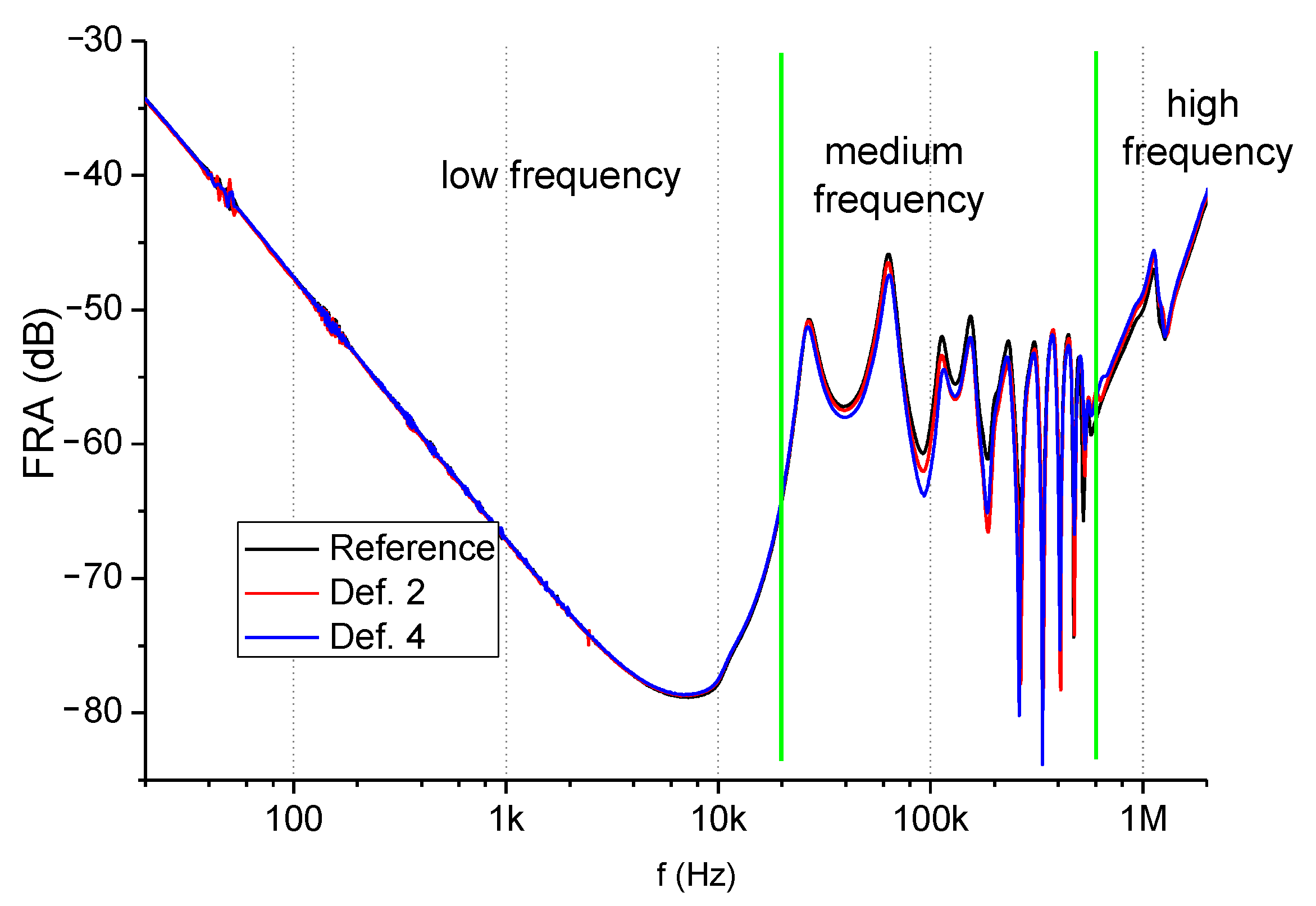
Another problem in using numerical indices is the selection of the input data. The authors use only a medium frequency (MF) range, in which local deformations in the windings would create visible differences. The borders of this range depend on the geometrical size of the transformer and its construction; generally, the bigger the transformer, the lower in the frequency domain its response lies. The low frequency range is strongly influenced by an iron core, so—for example—all short-circuits in windings can be easily detected, as they generate a large difference between the compared curves in this range. A high frequency range shows the influence of wave phenomena in the windings and the connection setup of the diagnostic equipment and is usually omitted in the analysis. Details of the selection of the borders for an MF range are described in [15] by authors of this paper and wider in doctoral thesis [16]; this starts with the inflection point on the capacitive slope of the first deep resonance (visible for an end-to-end open test circuit and being the result of interaction of the bulk capacitance of the winding with magnetizing inductance of the core) and ends with the beginning of the wave phenomena influence on the FR curve (visible as the character change of the curve)—the example is presented in Figure 1, which presents the FRA data measured on the transformer used for tests described in Section 3 of this paper (details of the measurement configuration are also given there).

Although the input data are limited to the MF range, is still too wide to allow GIM indices to performing an accurate analysis with just a single (global) value. The borders of this range should be used rather as the beginning and end of the assessment performed in narrower windows. The efficient comparative analysis necessary for FRA results assessment needs determination of the local differences between the curves: reference and analysed ones. In such a case, a “moving window” technique may be introduced. This is well known in digital signal processing and digital filtration algorithms, widely described in the literature (for example, see [17]). Similarly, the problems of digital signal quality assessment can also be found in many papers [18].

In this paper, the authors introduce the “moving window” technique to FRA data analysis with numerical indices. The research results presented in the article include:

• presentation of the assumptions of the FRA method,
• discussion of the properties of numerical quality criteria (numerical indices) used in the GIM method,
• assumptions of the “moving window” method applied to the analysis of numerical data obtained from FRA measurements,
• analysis of the probabilistic properties of four chosen quality criteria, taking into account the influence of the window size on the variance of the values of these quality criteria, and consequently—the impact of the window size on the readability of the FRA analysis results, and
• results of experimental research using a moving window and quality criteria used in the GIM method.

The data used for the analysis comes from controlled deformations performed on the active part of the distribution transformer and from industrial measurements coming from 10 MVA transformer. The aim of the research was to check the influence of a number of the window elements on the quality and applicability of a frequency response comparative analysis with chosen quality criteria.

2. Frequency Response Analysis and Assessment of Measured Data

In FRA results assessment usually only the amplitude is taken under investigation. It is commonly designated as FRA, so it can be written as follows:

FRA (dB) = 20log(U_out/U_in),

(1)

where U_in is the voltage on the input and U_out is the voltage on the output.

Differences between the curves can be observed as frequency shifts of resonances or changes in curve damping [19].

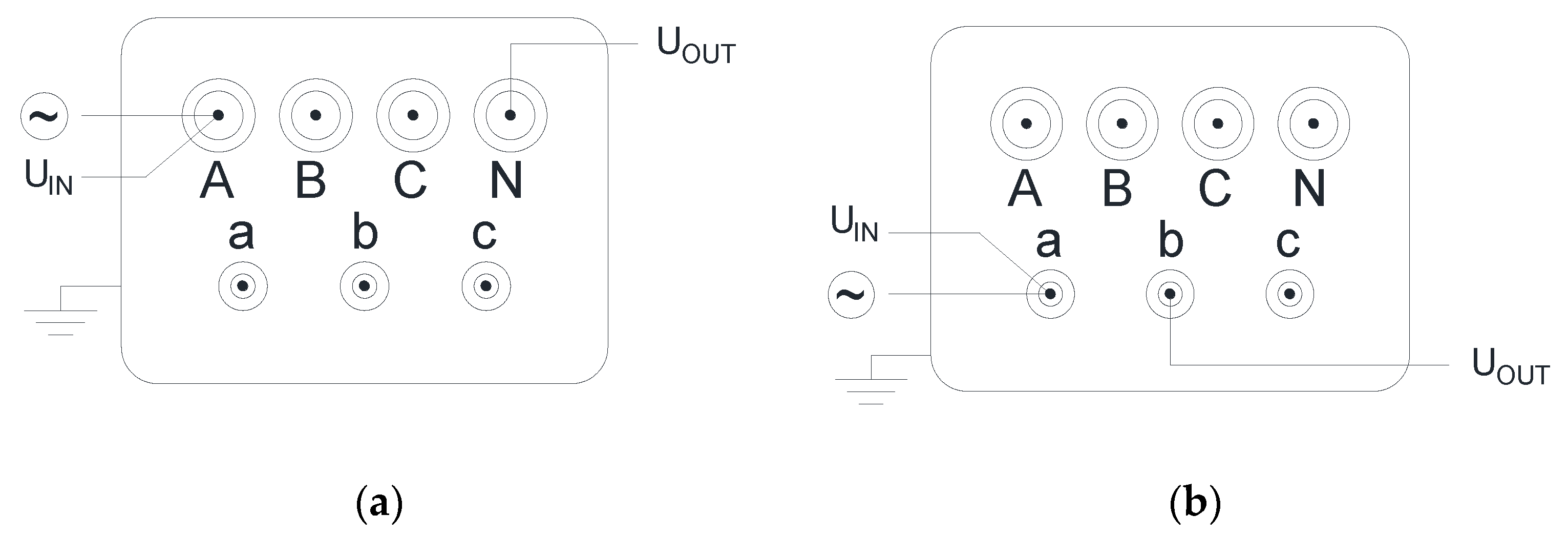
The FRA measurements methodology is standardized [20]. The standard provides details of performing the FR measurements to obtain repeatable results, allowing the comparison of test results measured by various diagnostic companies or by equipment coming from various producers. All measurement data used in this paper was obtained according to this standard and using the end-to-end open test setup, presented in Figure 2.

The FRA data was measured with a FRAnalyzer test device from Omicron (Austria), using standard settings, usually chosen by personnel for performing industrial measurements. This means that the total number of points, measured in the logarithmic scale of frequency (from 20 Hz to 2 MHz) was 1000. This number can be modified by advanced users, which allows for focusing on a given frequency range. These points are divided into frequency ranges as presented in

Table 1. Standard distribution of test points in frequency ranges for the Omicron FRAnalyzer test device.

From Frequency	To Frequency	Points	Sweep Mode
20 Hz	<100 Hz	50	logarithmic
100 Hz	<1 kHz	210	logarithmic
1 kHz	<10 kHz	210	logarithmic
10 kHz	<100 kHz	210	logarithmic
100 kHz	<1 MHz	210	logarithmic
1 MHz	2 MHz	110	logarithmic

.

FRA diagnostics using local assessment of quality indices is the actual scientific problem. The research in this field can be found in papers from top publishers [21,22] or from international conferences, for example [23]. An assessment based only on a single value returned by any numerical index may be misleading and result in a wrong interpretation of the measured FR data.

The application of the moving window technique generates a series of quality indices QI(f) (where f—frequency) for subsequent positions of the algorithm window. The values of QI(f) are calculated by a chosen quality criterion, for example MSE (mean squared error), CC (correlation coefficient), ASLE (absolute sum of logarithmic error) or SD (standard deviation) as proposed in the GIM method [10]. The formulas representing these indices are given in

Table 2. Numerical indices used in the grouped indices method (GIM) [15].

Name	Formula (Number)
Correlation coefficient	$CC=\frac{{{\displaystyle \sum }}_{i=1}^N{Y}_{0i}{Y}_{1i}}{\sqrt{{{\displaystyle \sum }}_{i=1}^N{\left[Y_{0i}\right]}^2{{\displaystyle \sum }}_{i=1}^N{\left[Y_{1i}\right]}^2}}$	(2)
Standard deviation	$SD=\sqrt{\frac{{{\displaystyle \sum }}_{i=1}^N{\left(Y_{0i}-Y_{1i}\right)}^2}{N}}$	(3)
Mean squared error	$MSE=\frac{{{\displaystyle \sum }}_{i=1}^N{\left(Y_{0i}-Y_{1i}\right)}^2}{N}$	(4)
Absolute sum of logarithmic error	$ASLE=\frac{{{\displaystyle \sum }}_{i=1}^N\left|20lo{g}_{10}{Y}_{1i}-20lo{g}_{10}{Y}_{0i}\right|}{N}$	(5)

.

The input values are two sequences of FRA measurement data: The reference FRA_Y0(f) = {Y0: y0_i | i = 1, 2, …, I}, and the diagnosed one, FRA_Y1(f) = {Y1: y1_i | i = 1, 2, …, I}, where I is the index of the subsequent element of the set and also index (number) of FRA test frequency. Regardless of used quality index F (Table 2), the analysis result—in general—will be a set QI(f) = {QI: qi_i|i = N < i < I − N}. Calculation of the elements of this set is performed by the general formula:

QI_i = F(y0_i−N<i<i+N, y1_i−N<i<i+N)

(2)

with the assumption that the algorithm window contains K = 2 N + 1 elements and N ≤ i ≤ I − N.

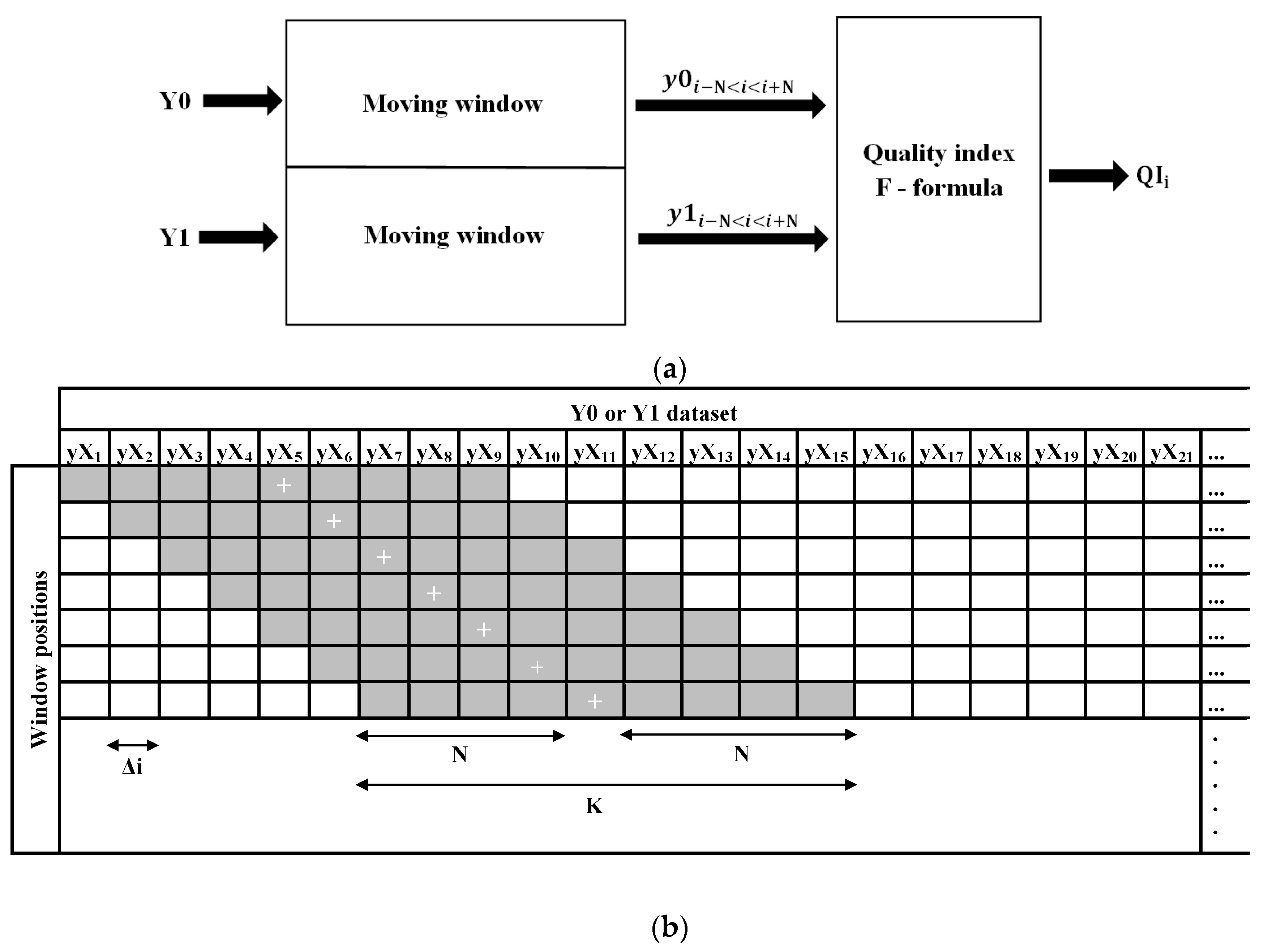
The process of QI(f) calculation is similar to an algorithm of Finite Impulse Response filter (FIR) with two inputs [4]. The input data are sets Y0 and Y1. The input data are used for the successive calculation of QI, according to the rule F, using the window containing K = 2 N + 1 of consecutive elements of data vectors (values Y0 and Y1)—see Figure 3a. The window is being moved along the input vectors by one element and in the calculation process there is created the vector of output data QI, containing 2∙N elements less than each of the input vectors. The process of selection of elements from input vectors, which are used for the calculation of QIi value is shown in Figure 3b.

The application of the moving window technique needs the determination of two parameters: a step of the algorithm and a number of window elements. If changes of index i are done with the step Δi = 1, the frequency resolution of calculated index QI(f) is maximal, equal to the number of measured points. If Δi > 1, the frequency resolution is lower.

The choice of the window size is not an easy task. It can be predicted that large values of K will lead to a smoothening of the results. On the contrary, the low values of this parameter would lead to a very precise QI representation of the differences between FRA_Y0 and FRA_Y1. In such a case, obtained result QI(f) may be hard to interpret, similarly to the raw input data (measured curves of FRA(f)). The question arises: what should be the value of K?

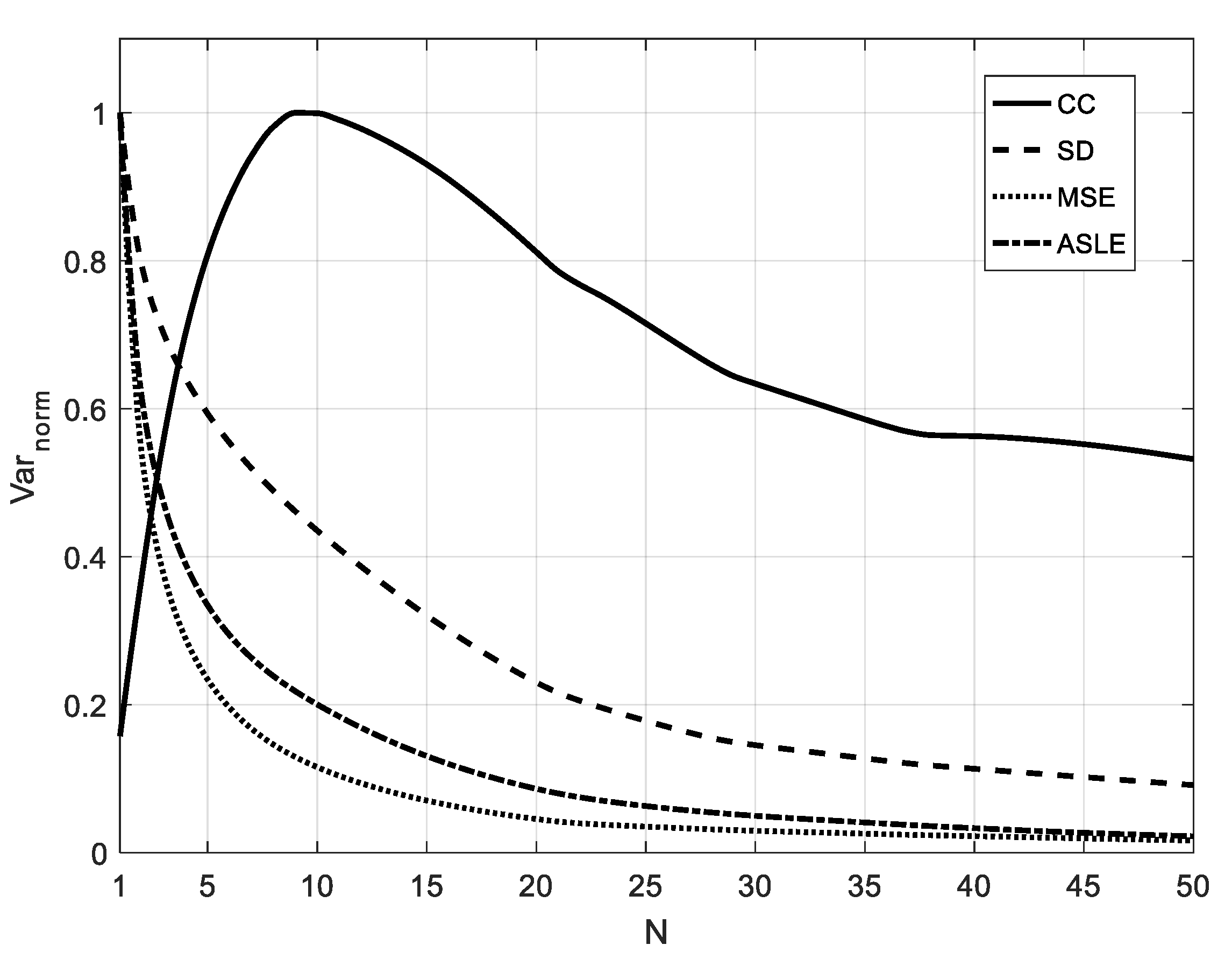
If all probabilistic properties of the FRA dataset are taken under consideration, as well as the definitions of the chosen quality indices CC, SD, MSE and ASLE, the dependency of the indices variance changes as a function of N parameter (defining the number of window elements K = 2 N + 1) are given in Figure 4. The vertical axis represents—normalized to maximal values—the variance of the chosen quality indices. It can be seen that in the case of SD, MSE and ASLE, the application of a small size window would lead to a precise representation by these indices of the changes between the reference and diagnosed FRA datasets. For windows having large number of elements (e.g., with K > 11 (N > 5) elements), the curves representing these indices value changes would be smoothened, which in FRA diagnostics—in some cases—may be advantageous.

The variance values for each QI quality index (CC, SD, MSE or ASLE) were calculated using the definition of unbiased estimation of variance:

$$Var\left(\mathrm{QI}\right)=\frac{1}{\mathrm{L}-1}{\displaystyle \sum }_1^{\mathrm{L}}{\left({\mathrm{QI}}_{\mathrm{i}}-\overline{\mathrm{QI}}\right)}^2$$

(3)

where:

QI_i are the values of CC, SD, MSE or ASLE calculated for all positions of the window having K = 2 N + 1 elements, “shifted” along the input data vector according to formula (6), which contains L elements, 1 ≤ i ≤ L,

$\overline{\mathrm{QI}}$ is the mean value of CC, SD, MSE or ASLE, calculated for given window size K = 2 N + 1.

Finally, for such calculated vectors of variance (separately for individual quality indicators), graphs shown in Figure 4 were prepared, normalizing the results against the maximum QI value for each of the quality criteria.

A different character of window size influence on variance may be observed for the index CC. A maximum can be clearly seen on its graph in Figure 4. This means that for the N equal to approximately 10 the variance of CC index values is maximal, which results in the most exact representation of its changes in the frequency function. The curves shown on Figure 4 were obtained by averaging the results of the normalized variances calculations of four quality criteria for eight transformers (which have various power ratings) and for the standard measurement point distribution in frequency ranges, as shown in Table 1. If the frequency spectrum will be divided in a different way, the maximum value of CC index normalized variance is for N different than 10. In the case of the remaining indices curves would be similar to those presented on Figure 4 and will still be valid for the rule: “small” window—big variance, “large” window—small variance.

The conclusion from this comparison is that the optimal value of N cannot be defined. It depends on the expected final effect: a very exact representation of the changes or a smoothened analysis result. In the first case for three criteria: SD, MSE and ASLE, the value of N shall be lower than 5 (the increase of the variance in Figure 4). Where the analysis results need smoothening, it is the contrary. A significant increase in the value of N (much more than 5) will not influence the quality of the results: the smoothening level will change slowly, while the amount of calculations will change proportionally to the number of elements in the algorithm window.

In the case of the CC index window width estimation, the character of its variance changes needs to be considered in the function of N. A choice of N = 10 would allow for detailed representation of its values changes in the frequency domain, so its “sensitivity” would be maximal (for a standard distribution of test point in frequency ranges given in Table 1).

3. The Influence of the Window Size on GIM Indices

The four indices, chosen for the GIM method, were used for assessment of the data coming from the deformational experiment, performed on a 6/0.4 kV, 800 kVA, Dyn transformer. Its active part was removed from the tank and various deformations were introduced into windings. One of them was chosen for testing the abovementioned indices with different sizes of analysis window. The results measured in controlled deformations are especially useful for described numerical indices analysis, because they are connected to a known deformation in the winding. This deformation was based on compression of the top disks, by removing spacers between them—it is presented in Figure 5. It was applied to disks 1-2 (Def. 1), 1-3 (Def. 2), 1-4 (Def. 3) and 1-5 (Def. 4), so there were four levels of this deformation, compared to the reference measurement.

The analysis of the four GIM indices was conducted in the medium frequency range, which for this transformer was set from 20 kHz to 600 kHz (according to [15,16]). Various values of N were analysed. In the following section, three of these are presented in the graphs: N = 1, 10 and 20. The presentation of more results would make the graphs unclear.

Figure 6 presents the FR data measured on this unit and used for the analysis. The graph shows only the MF range, used for further analysis (it is a part of curves from Figure 1). At the lower and higher frequencies no significant changes between the curves are present. To make the graph clear, only two deformations are presented (Def. 2 and Def. 4) with the reference curve (healthy winding). The differences between the curves are visible as damping shifts of the whole frequency ranges (for example from 70 kHz to 200 kHz) or at the resonant points (270 kHz, 340 kHz, 470 kHz).

Figure 7, Figure 8, Figure 9 and Figure 10 present the values of the four numerical indices for various values of N (K = 2 N + 1). Each case also contains the average value, which is a single value calculated from the given index for the whole analysed range. In other words, it represents the typical industrial approach to analysis with numerical indices and is presented on the graphs with dashed line. The curves used for comparison with the indices are the reference one and Def. 4—the biggest deformation.

It is expected that with the increase of the value of N, the graph will get flattened. The cause of such behaviour is illustrated in Figure 4: for the large values of N, the variance of the indices values decreases, so the smoothening level gets higher.

The first example (Figure 7) is calculated with the ASLE index. The differences between N = 1 and N = 20 are clearly visible, especially in the frequency range where a narrow and steep value change appears—for example at approx. 270 kHz or 340 kHz. The smoothening is very strong, if compared to less steep areas (for example at approx. 100 kHz).

The next graph (Figure 8) presents the calculation conducted with the MSE index. In this case, the graph flattening is also very strong in the case of narrow and steep areas, such as at approx. 270 kHz. The difference between the average value (dashed line) and the maximum value for N = 1 is huge.

Figure 9 presents the results of assessment with the SD index. The conclusions are similar to the two previous cases, however, the smoothening is not so radical with the increase of N elements. For example, at approx. 270 kHz the change of the window size from 3 (N = 1) to 21 (N = 10) results in the drop of the SD value by approximately half.

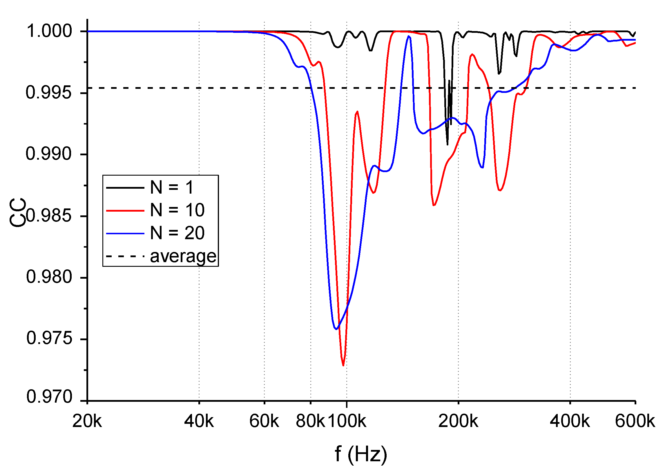
The last example is the values of the CC index, shown in Figure 10. For this numerical index, the influence of the number of N is not so obvious.

Depending on the frequency range, the number of N influences to a different extent. For example, the resonance of the FR data at 270 kHz gives the biggest change to the CC result if the value of N = 10, while the two other resonances (340 kHz, 470 kHz) give the biggest change in CC for N = 1. This is related to the width of the resonance (see Figure 6), as the first of these (270 kHz) does not have slopes as steep as the other two.

To summarize the results from Figure 7, Figure 8, Figure 9 and Figure 10, it can be stated that the window size depends on ones needs, whether it is necessary to smoothen or sharpen the output curve. However, the best value for the average approach is N = 10—especially in the case of CC index. For this quality index the value N = 10 guarantees the optimal precision of local values changes representation (Figure 2), which advantageously influences the legibility of CC (f) curve and the accuracy of diagnostic conclusions. In order to compare indices ASLE, SD, MSE and CC this value is used for testing all the indices for various extents of the deformation, which is presented in Figure 11, Figure 12, Figure 13 and Figure 14. The curves presented on these graphs are the results of the assessment of the FR data with the four indices. Each curve represents the values calculated from comparison of the data measured in the healthy state with the data measured after introducing the deformation. For example, the curve marked as Def. 1 is the result of analysis with a given index, for N = 10, of the reference line and the line for deformation 1. Figures contain the results for Def. 1, Def. 3 and Def. 4 (minimal deformation, maximal deformation and one in-between) to make them easier to analyse. In addition, for each case the global value of the given index is given, in other words the average value, for the window width equal to the total number of points in the analysed MF range.

The first example is shown in Figure 11, presenting the results obtained with the ASLE index. Depending on the frequency range (input FR data), there are visible various behaviours of curves calculated for the three deformation scales. However, if these shapes are compared to the global values (for the whole range), which are Def. 1—0.140, Def. 3—0.225 and Def. 4—0.230, it can be seen that latter two do not reflect the complexity of the changes visible on the graph, where—for example—Def. 3 has its maximum at 180 kHz, while for Def. 4 it is at 240 kHz. Their global values are almost the same, so an analysis based on them would not show any differences between these two cases. In other words application of the moving window technique is proven to be effective in the analysis of the FRA data.

A similar effect can be observed in Figure 12, where the MSE index was used for the assessment. The global values are in this case: Def. 1—2.92, Def. 3—5.11, Def. 4—5.04, so, again, the latter two are almost similar, while the curves show the maximums for different frequencies. The same conclusions may be drawn for the third index, SD (see Figure 13), where the global values are, respectively: 1.71, 2.26 and 2.25.

The last case, the CC index, also has similar behavior. Def. 1 has its maximum at approx. 540 kHz, Def. 3 at 340 kHz, while Def. 4 is at 270 kHz. In this case, the global values are: 0.99961, 0.99944 and 0.99945, so again Def. 3 and Def. 4 are very similar—see Figure 14.

From the above examples, it can be seen that for N = 10 all four indices act in the same way: their local extremums depend on the actual deformation and its influence on the FR curve. The comparison to global values clearly shows that analysis done for the narrower window, not for the whole analysed range, gives more information. It can be seen that for deformations introduced into the winding, the global value of the quality index may be insufficient to detect the fault. The quality indices for Def. 3 and Def. 4 are almost similar, while the measurements were taken for different geometries of windings.

4. The Application to Industrial FRA Results

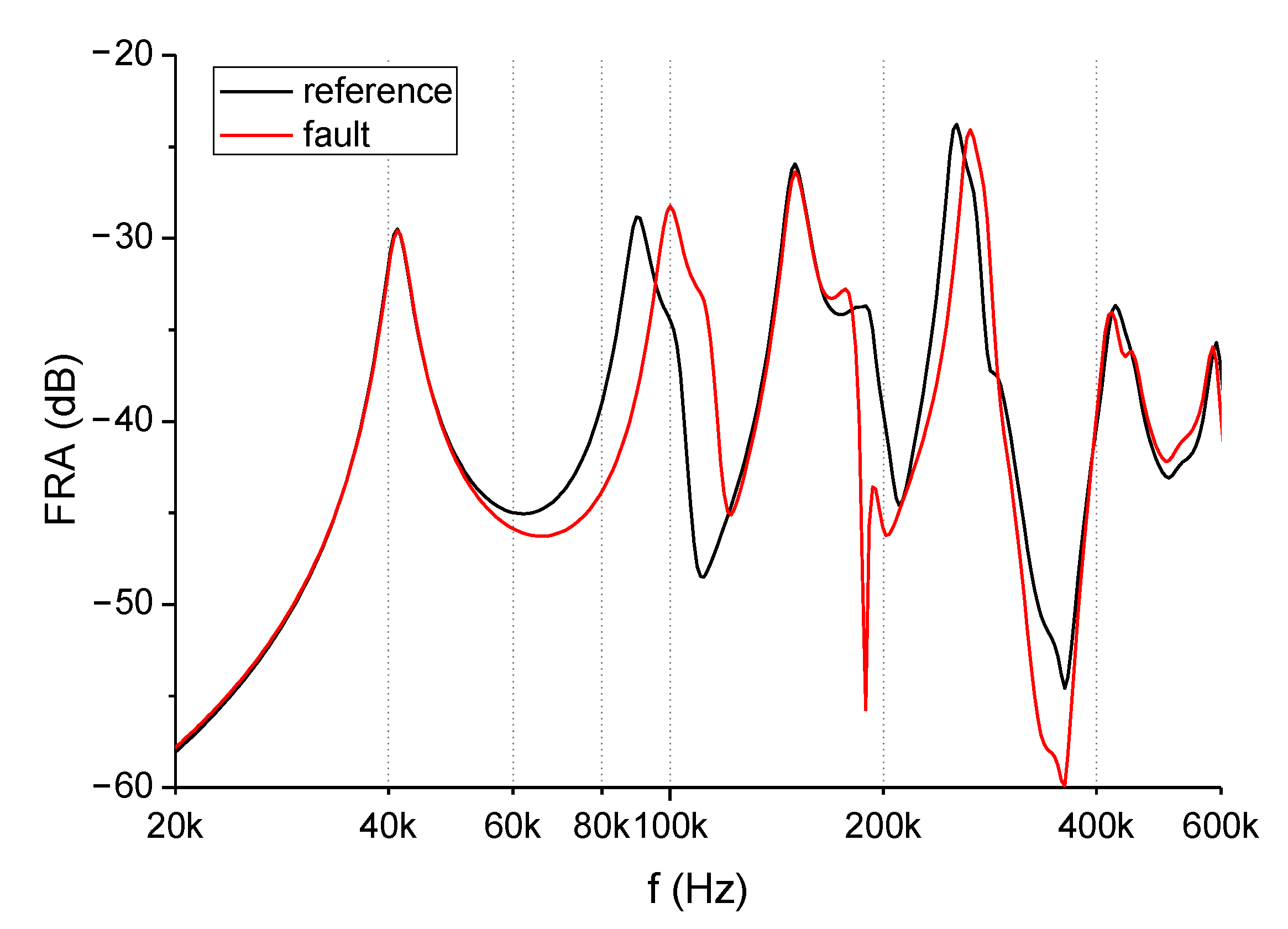
The research described in the Section 3 was repeated for data coming from the industrial measurements. The tested transformer was 15/6 kV, 10 MVA unit, which has clearly visible differences between two measurements, namely reference and fault curves. The medium frequency range, which in this case is from 20 kHz to 600 kHz, can be observed in Figure 15. The exact cause of differences seen on this Figure is unknown for the authors, because the owner of the transformer did not share decisions taken on transformer further operation and possible results of the internal inspection. However, these results are good for the moving window technique analysis, because differences between both curves cover all possible scenarios, which can be encountered in the transformers’ frequency response analysis: a shift in the frequency domain (60–120 kHz) related to capacitance changes, a change of a shape with a new resonance (approx. at 200 kHz), which can be affected by many factors that constitute that parallel resonance (e.g., capacitance and inductance interaction in that frequency) and a damping change (approx. at 360 kHz) being an effect of changed parameters forming given resonance, e.g., capacitance and turn-to-turn magnetic couplings, if there was a deformation in the winding or local resistance change in the case of partial (via small resistance) local short-circuit. With such data the comparison of changing window widths showed all possible behaviours of the output data.

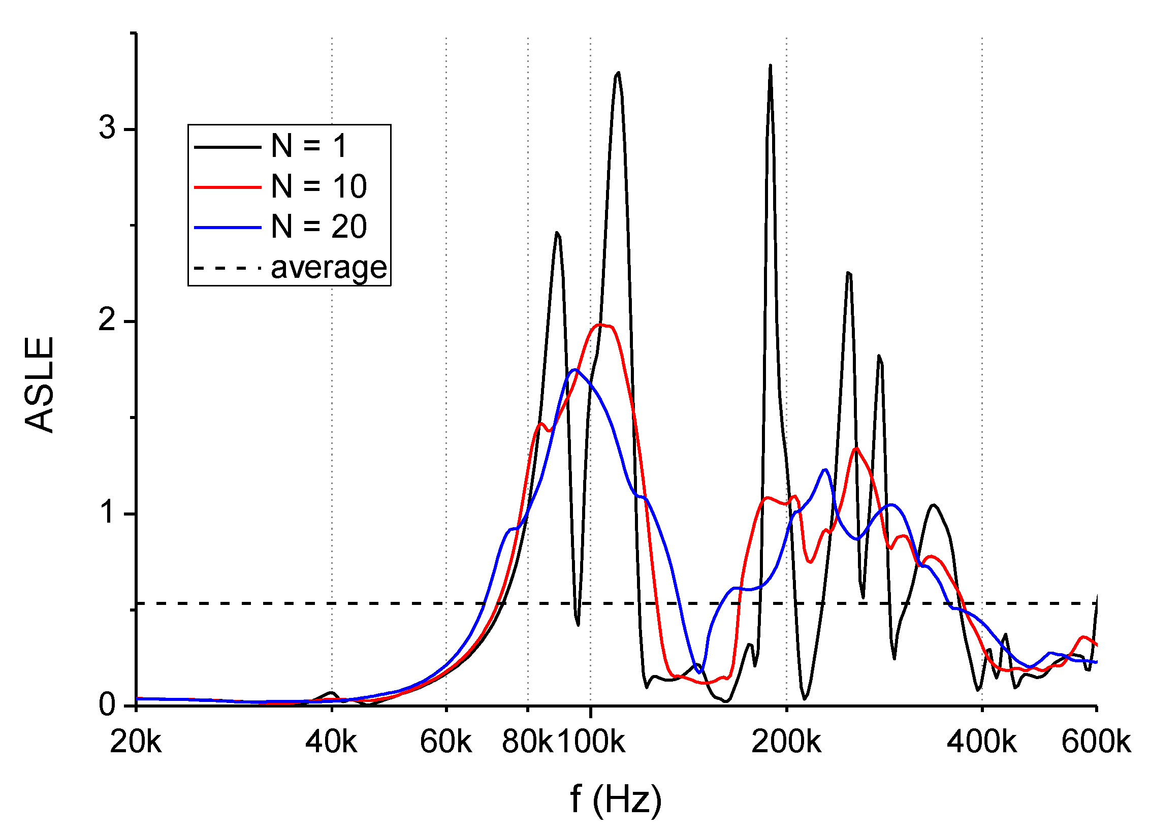
The first tested numerical index was ASLE. Its results are shown in Figure 16. For value N = 1 the output results are very sharp, strongly pointing all present differences between curves. By increasing the N value to 10 and 20 the curve is smoothened and follows the frequencies of changes visible in FR graph from Figure 15. For diagnostic purposes the better result is obtained for value N = 10, because for changes at 200 kHz and 360 kHz is shown two separate maximums. Additionally, if compared to the average value, used in the standard approach to numerical indices application, there are clearly visible frequency ranges in which curves vary from this value.

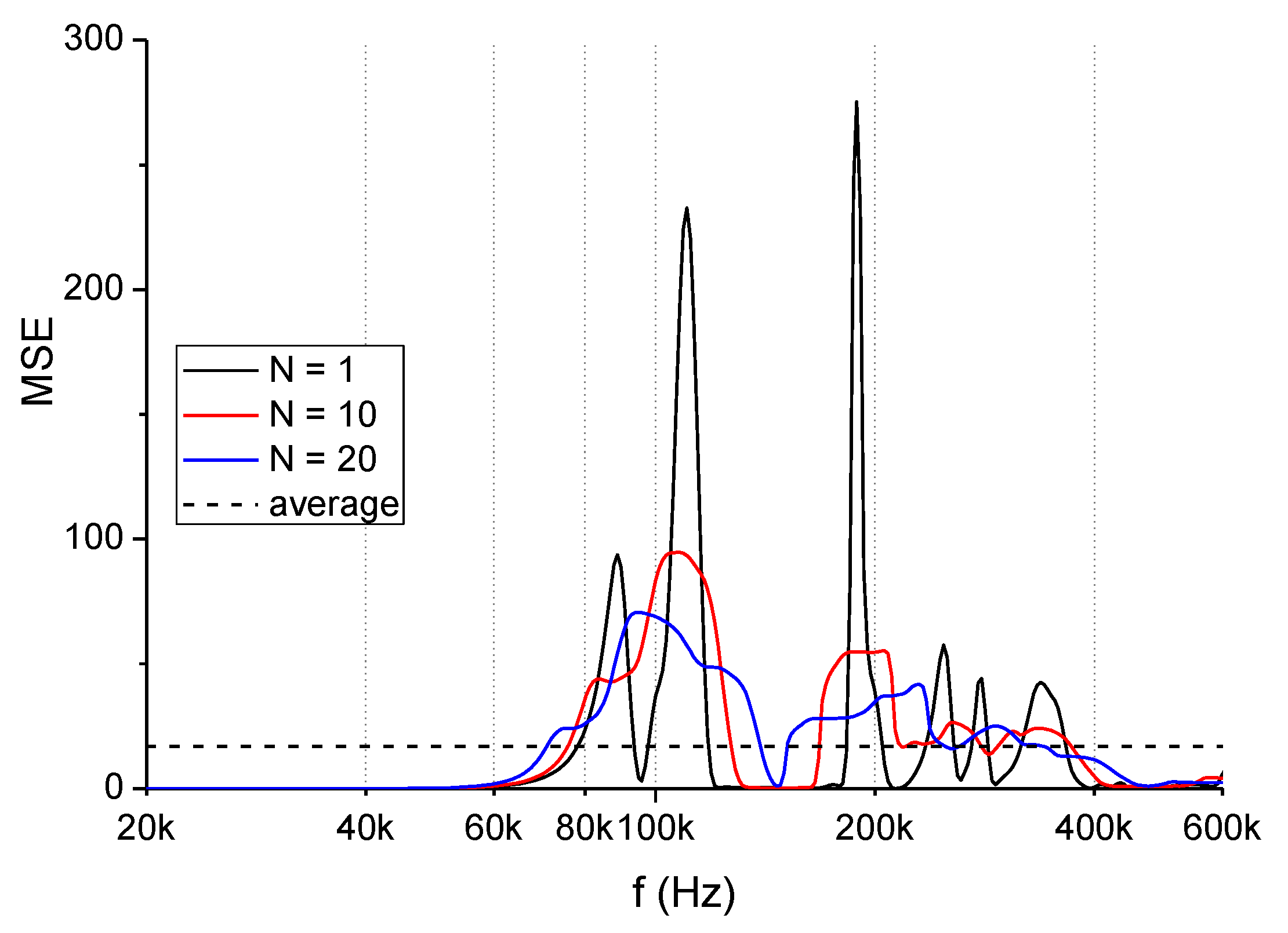
Similar conclusions may be drawn for data presented in Figure 17 and representing the assessment with MSE index. For N = 1 the output graphs reaches very high amplitudes and is strongly sensitive on any differences between two input curves. Again, for N = 10 some local maximums may be observed in frequency ranges correlating to FR curves measured on the transformer and comparison to the average value clearly indicated “suspicious” frequency ranges.

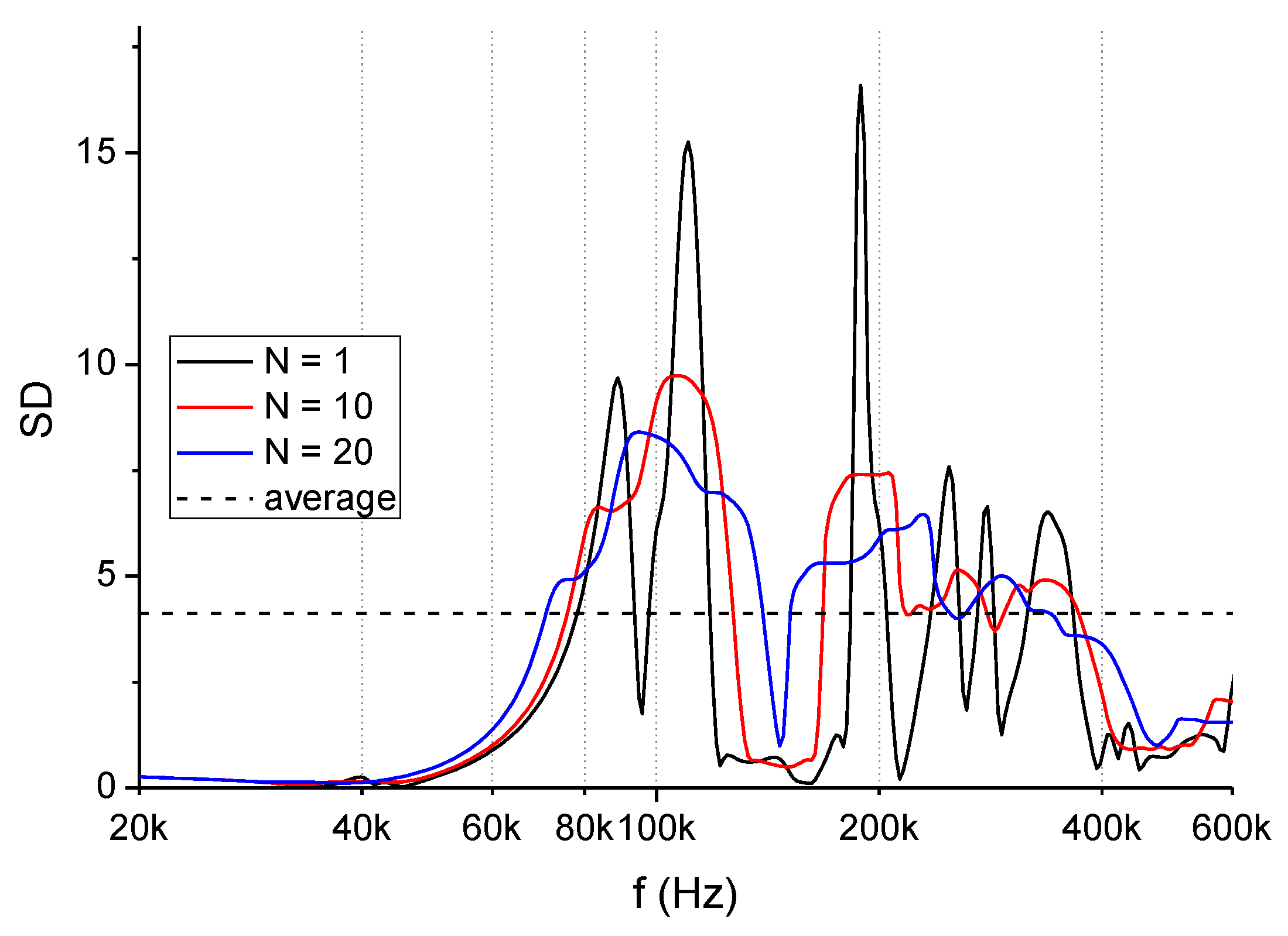
The third numerical index is SD, with results for various window sizes presented on Figure 18. Also this case shown the best efficiency in the detection of differences between input curves for N = 10, both indicating frequency ranges connected to faults and giving the good contrast if compared to the average value (global).

The last case is CC numerical index, analysed in Figure 19 and showing different behaviour. The value N = 1 gives the smaller sensitivity to differences between input curves, pointing out mainly the change of the shape (new resonance). However, the increase of N to 10 or 20 returns more differences in the curve shape. Additionally, in this case N = 10 gives better results, because the index is more sensitive to local changes. For example there are visible local minimums at approx. 200 kHz and 250 kHz. All such local “suspicious” frequency ranges differ from the average value of this index.

The analysis of results presented on Figure 16, Figure 17, Figure 18 and Figure 19 leads to the conclusion that the best quality of detection of differences between compared curves is achieved for the value N = 10, for which all categories of changes are indicated in the graphs: resonance shifts, damping changes and curve shape change.

5. Summary

The paper presents the research on the data window width for the analysis of frequency response results of transformer windings performed with numerical indices. Four quality indices were chosen to test the results measured on the active part of the transformer with deformations introduced into the winding. The results were analysed for various window widths (K = 2 N + 1).

In the first stage, the variance of the four indices was tested, depending on the N value, which allowed for testing their sensitivity to this parameter. In the case of the correlation coefficient (CC) index, the results were not unequivocal.

The analysis of data for various extents of deformation introduced into laboratory tested transformer showed that the approach based on moving the window is more accurate and allows for detection of the winding geometry changes, which are undetected by a standard approach with a single (global) value of a given index. This is clearly presented in the case of deformations 3 and 4. The choice of the N value depends on the needs of the analysis, however, the proposed N = 10 seems to be the most universal and useful for most practical analyses, however, some users of the frequency response analysis (FRA) method may need other effects (smoothening vs. sharpening). The similar conclusions may be drawn from observation of the industrial measurements performed on the second transformer. The value N = 10 allowed for the best effect of differences detection between compared frequency response curves (datasets). For such value the output curve of each numerical index clearly showed the local difference of the value, strongly differing from the average value, for any type of possible changes to the output data: a frequency shift, damping change or change in the shape (new resonance).

For practical application of obtained results authors propose to compare output data of each index in frequency range for N = 10 to average value (local maximum to average value ratio). By setting the fault detection criteria, for example on level 30%, it will be possible to identify the frequency ranges of input frequency response data having “suspicious” values differences. It can be applied to the automatic detection systems. The results of experimental tests presented in Section 3 relate to an exemplary transformer with a power rating of 800 kVA. It should be clearly emphasized that the proposed “optimal” window sizes apply to transformers with such power and design features and—in particular—with the adopted frequency resolution of the frequency response analysis method.

The value of fault detection criteria should be further analysed, because it depends for example on geometrical size of the unit (power rating) or its construction. This topic is the subject of further research of the authors. In this paper, the authors wanted to draw the attention of other researchers dealing with diagnostics using the frequency response analysis method to the problem of window size selection when using objective (numerical) quality indicators. The readability of the obtained results for local frequency ranges depends on the number of window elements and there is no intuitive rule: the precision of mapping local numerical changes in quality indicators is inversely proportional to the number of window elements. This is evidenced by the presented analysis of the variance of changes in the correlation coefficient value, for which the maximum variance occurs for a given number of window elements.