Abstract
Site Index has been widely used as an age normalised metric in order to account for variation in forest height at a range of spatial scales. Although previous research has used a range of modelling methods to describe the regional variation in Site Index, little research has examined gains that can be achieved through the use of regression kriging or spatial ensemble methods. In this study, an extensive set of environmental surfaces were used as covariates to predict Site Index measurements covering the environmental range of Pinus radiata D. Don plantations in Chile. Using this dataset, the objectives of this research were to (i) compare predictive precision of a range of geostatistical, parametric, and non-parametric models, (ii) determine whether significant gains in precision can be attained through use of regression kriging, (iii) evaluate the precision of a spatial ensemble model that utilises predictions from the five most precise models, through using the model prediction with lowest error for a given pixel, and (iv) produce a map of Site Index across the study area. The five most precise models were all geostatistical and they included ordinary kriging and four regression kriging models that were based on partial least squares or random forests. A spatial ensemble model that was constructed from these five models was the most precise of those developed (RMSE = 1.851 m, RMSE% = 6.38%) and it had relatively little bias. Climatic and edaphic variables were the strongest determinants of Site Index and, in particular, variables that are related to soil water balance were well represented within the most precise predictive models. These results highlight the utility of predicting Site Index using a range of approaches, as these can be used to construct a spatial ensemble that may be more precise than predictions from the constituent models.
1. Introduction
Pinus radiata D. Don (radiata pine) is the predominant plantation species within Chile and there is considerable interest within the forest sector in the accurate prediction of Site Index for this species [1]. P. radiata is the most widely established plantation species within the Southern Hemisphere, and this species constitutes a large proportion of plantations in Chile, New Zealand, and Australia [2]. This species is very responsive to environment and, as a consequence, productivity has been found to range widely across the environments over which it is grown [3,4]. A number of process-based models, such as 3PG [5], CenW [6], and CABALA [7], have been developed to describe how the environment influences growth of plantation species, such as P. radiata (e.g., Kirschbaum and Watt [8]). However, empirical or hybrid models are still the most widely used for predictions of plantation productivity, as these models are simpler to parameterise and can provide more precise estimates of growth than process-based approaches [9].
Stand productivity is modelled by empirical models as a function of stand age, while using non-linear functional forms. Variation in the productivity between stands is accounted for by standardised measurements of productivity at a given age that are used to adjust both the trajectory and the asymptote of predictions of productivity over time [10,11,12]. Site Index, which expresses the height of dominant or co-dominant trees at a reference age [13], has been most widely used to account for this inter-stand variation, as this metric is correlated with productivity [14,15] and the height of dominant trees is relatively invariant to stand density [16,17,18].
Environmental surfaces have been widely used through a range of modelling approaches to develop maps of Site Index for P. radiata [3,19] and many other coniferous tree species [20,21,22,23,24,25]. When compared to direct measurements of Site Index made using plot data, which are typically averaged to the stand level, predictions of Site Index from environmental surfaces open up a range of applications that are not available from traditional inventory. The resulting spatial description of Site Index provides insight into the key environmental drivers of productivity and allows for managers to understand how productivity is likely to vary across the landscape and where the optimal productivity will occur at a range of resolutions from the intra-stand to the regional level [3,19]. In contrast to spatial predictions of Site Index from remotely sensed data, such as LiDAR, [26], surfaces of productivity, which are created from environmental surfaces can also be used to estimate productivity for unplanted areas, providing managers with insight into the potential value of land that they intend to purchase [27].
The use of Site Index surfaces to parameterise empirical growth models incorporates elements of process-based modelling, as Site Index integrates the most important determinants of tree growth, including topography, soil characteristics, and climate [28]. Consequently, spatial predictions of Site Index provide a means of generating stand growth curves that are sensitive to fine and coarser scale landscape level changes in climatic and edaphic conditions [29]. These estimates of stand development allow for managers to spatially optimise the timing of a range of silvicultural operations including thinning and pruning, across their estate [30,31]. The site Index surfaces can also be used as input to models that are used for key management decisions, such as the optimisation of final crop stand density (S) and the development of surfaces showing spatial variation in S [32].
A large number of modelling methods with varying levels of complexity have been used to predict Site Index for a wide range of forest species growing in Europe, North America, and New Zealand. These methods range from relatively simple approaches, such as multiple linear regression [4,21,22,23,24,25,33,34,35,36,37,38,39,40,41,42,43,44], to more complex parametric methods, such as Partial Least Squares, Lasso, Elastic Net, Least Angle Regression, and Infinitesimal Forward Stagewise Regression [45]. A wide range of non-parametric methodologies has also been used to model Site Index, which includes Random Forests [46,47], Boosted Trees [33,34], Classification and Regression Trees [33,34], Neural Networks [34], Generalised Additive Models [33,34,48], and Multivariate Adaptive Regression Splines [45].
Parametric methods that utilise the spatial correlation between the underlying plot data describing Site Index have been less frequently used to develop models and surfaces of Site Index. Amongst these geostatistical methods, ordinary kriging and regression kriging are the most commonly used techniques [3,19]. Because predictions are made by ordinary kriging through interpolating values between measured plots, this method is most precise when plots are located in relatively close proximity [3]. Regression kriging is less reliant on a dense plot network than ordinary kriging, as this method fits an underlying regression model and then geospatially refines these estimates through kriging the model residual variation across the area of interest [3].
The recent emergence of advanced machine learning methods allows for greater utilisation of the increasing amount of information in geospatial surfaces, as these models can often accommodate collinearity between closely correlated environmental variables [49,50]. Despite this advantage, few studies have compared the predictive precision of these methods with more traditional approaches. For forest species located in Belgium and Turkey, Site Index was more precisely predicted while using non-parametric methods than multiple linear regression and, amongst non-parametric methods, artificial neural networks had the highest predictive performance [33]. Comparative studies of model performance undertaken in P. radiata plantations have highlighted the precision of regression kriging and more advanced non-parametric models, but, as with other forest species, have not included a comprehensive comparison of the models. Within New Zealand plantations, regression kriging was found to be marginally more precise than ordinary kriging, which, in turn, was more precise than Partial Least Squares [3,19]. A comparison of seven modelling methods using data that were collected from northwest Spain found the non-parametric Multivariate Adaptive Regression Splines (MARS) to be the most precisely predicted Site Index, which was closely followed by the parametric methods of stepwise regression and PLS [45].
Because each modelling method has its own limitations and advantages [51], an alternative approach for improving the overall model precision is to combine predictions from each model [52,53]. This method, which is known as Ensemble Modelling, is a well known methodology that can improve prediction through integrating knowledge from many sources [53]. Although this technique has been used for the prediction of many soil attributes [53,54] and class prediction studies [52], we are unaware of any studies that use spatial Ensemble Models for the prediction of Site Index.
In Chile, different Site Index curves have been developed for each region and geographic area, although these local predictions are relatively inaccurate and there is little understanding of how the Site Index responds to topography, climatic and edaphic conditions [55]. Given the wide diversity of environmental conditions within the region over which plantations are grown, we assumed that more than one modelling method would be required to best predict Site Index across south-central Chile. Consequently, the objectives of this study were to compare the precision of a wide range of modelling algorithms and determine whether the combination of multiple algorithms (e.g., by the means of spatial ensemble learning) could more precisely predict Site Index than the best performing single modelling algorithm.
2. Materials and Methods
2.1. Data and Covariates Description
Stand level data describing Site Index of P. radiata were extracted from 20 year stands. The site index for P. radiata is defined as the mean top height at age 20 years old, where mean top height is defined as the mean height of the 100 largest diameter trees [56]. As stands used in this study were planted between 1987–1997 Site Index could be estimated at 20 years of age rather than being projected forward to 20 years as is commonly done [57]. In total, there were 64,190 observations of Site Index available for modelling that were dispersed from Región del Maule (latitude ) to Región de los Ríos (latitude ) and covered a Site Index range of 14.2–42 m with a mean of 29.0 m. These observations were randomly split, with 75% used for the fitting dataset, 12.5% for the calibration dataset (used for the ensemble methodology only), and 12.5% for the validation dataset. All three datasets covered a similar geographic range that was representative of the location of P. radiata plantations through Chile (Figure 1). The site Index and enviromental conditions were very similar between the three data sets, and they are summarized in Table 1.
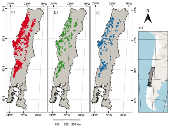
Figure 1.
Map of the spatial distribution of observations, showing the location of (a) fitting (n = 48,117), (b) calibration (n = 8036), (c) validation (n = 8037) data sets and (d) Delineation of the study area within the Chilean territory.

Table 1.
Site variation in climatic variables and Site Index for the fitting, calibration and validation data sets. The values shown represent the mean, followed in brackets by the range.
The 64 environmental factors or covariates, as listed in Appendix B, were extracted for each of the plot locations at a 90 × 90 m resolution from spatial layers. These spatial layers described topography, vegetation index, soil properties, and climate. Topography was characterised from a Digital Elevation Model (DEM) that was created using LiDAR. Automated Geoscientific Analyses (SAGA) was used to extract the topographical variables listed in Appendix B from this DEM. The enhanced vegetation index (EVI) was used in order to characterise the vegetation. The values for EVI were derived from MODIS images collected between 1987–2017 period that were reclassified to 90 × 90 m. Values of EVI describing the mean, range, and standard deviation were extracted from this imagery (Appendix B). The soil morphology was determined from the Chilean Natural Resources Information Center (CIREN). The soil properties were determined by interpolating data from ten thousand soil pits that were distributed across south-central Chile that belong to Arauco. The soil surfaces available from this dataset included soil depth, clay content, nutrient content (C:N ratio, N content) and physical properties (available soil water, bulk density, hydraulic conductivity). Long term monthly air temperature, rainfall, evapotranspiration, and water balance were obtained from CR2 (Center for Climate and resilience research [58]), which is unpublished information, but available for purchase.
In addition to long term averages, mean climatic data that were linked to the time period of each plot were also used within analyses. These covariates were developed for the model prediction while using the climate that was experienced by each forest stand (observations), from the plantation establishment until an age of 20 years, including the effect of rainfall for different stand periods (first, second, and forth initial years post establishment), accumulative cold days, evapotranspiration, and water deficit index per stand. Where these variables were significant based on the relative environmental feature selection (details in Section 2.2), they were used to construct the models. The map development used raster surfaces of these variables while using the average values over the last 30 years for air temperature, water balance, rainfall, and evapotranspiration.
2.2. Subsetting of Covariates for the Modelling
A pre-processing method was used in order to extract a subset of relevant features from the available 64 covariates. According to Weston et al. [59], this step plays an important role in improving prediction performance and can reduce overfitting. Two types of redundant features selection were made. The first was for non-parametric models (NPM), which included random forest (RF), support vector machines (SVM), neural network (ANN), eXtreme Gradient Boosting (XGBoost), and Multivariate Adaptive Regression Splines (MARS). The second method was used for parametric models (PM), including multiple linear regression (MLR), partial least squares (PLS), and elastic net (EN). Appendix A provides the description of the pre-processing that each of these models follow. Using the methods detailed in the next subsections, a total of 18 variables were selected for PM, while 20 were selected for NPM. From these selected ’optimal’ variables, the top five were identified based on their level of importance ranking, while using the mean reduction in accuracy (MDA) for NPM (further details in Section 2.1) and Pearson correlation coefficient for PM. The models of Site Index were developed while using PM and NPM methods that were based on both the optimal selection and the top five variables. Model development using the reduced number of variables was undertaken in order to produce a greater computational time efficient alternative, interpretable, and parsimonious models, and to explore how variable number affected statistical differences in SI prediction.
2.2.1. Covariate Selection for Non-Parametric Models
Recursive Feature Elimination (RFE) implemented via caret [60] was used to subset variables for the NPM. This method seeks to improve generalization performance through removing the features that have the least effect on training errors [61]. RFE is basically a backward selection of the predictors, which selects features by recursively considering smaller and smaller sub sets of features, and then builds a model while using the remaining attributes and calculates model accuracy with an internal cross-validation [62].
During the reduction of input selection with RFE the importance of each variable is measured based on the MDA. This process assesses how much the prediction accuracy drops by randomly permuting the values of each input variable (one at a time). A higher importance of the input variable under consideration corresponds to larger reductions in the prediction accuracy [63]. The top five covariates were selected based on RFE importance level.
2.2.2. Covariate Selection for Parametric Models
A penalized regression was used in order to reduce the number of predictors for PM as this method has been shown to produce more parsimonious models [64]. A least absolute shrinkage and selection operator (LASSO) was used to penalize the parameter estimates to avoid overfitting. LASSO finds the best variables and coefficients by minimizing the residual sum of squares and adding penalties that are useful for fitting a wide variety of linear models [65]. This technique requires the selection of a tuning parameter that determines the amount of shrinkage.
This method was followed by a complementary collinearity test while using the variance inflation factor (VIF). VIF can be used in order to identify correlated variables, which can inflate coefficient values, and it is determined from the following formulation [66],
where is the coefficient of determination.
The variables that were identified to be most important by penalized regression were reduced to a set of 18 predictors while using a procedure that sequentially eliminated correlated variables with a VIF that exceeded four [66].
After LASSO and VIF were completed, a ranking of the variables was obtained that was based on the strength of the regression between the variable and Site Index.
2.3. Modelling Approach
2.3.1. Overview
Five types of modelling methods were used in order to predict Site Index. Each of them used various machine learning and regression algorithm methods, which included: (1) geostatistical models (ordinary kriging [3,19]); (2) parametric models (multiple linear regression, partial least squares [45], elastic net); (3) non-parametric models (random forest [67], support vector machines [62], neural network [33], XGBoost [68] and MARS [45]); (4) hybrid models (random forest-kriging and PLS-kriging [19]); and, (5) a modelling ensemble approach using the best five models from the previous four categories. The strategy for fitting the models is outlined below. The parametric, non-parametric models and ordinary kriging (OK) were fitted to Site Index while using the fitting dataset. Regression kriging was then used to create a range of hybrid models from the fitting dataset, through kriging the residuals of the partial least squares and random forest models. Predictions from all of these models were then made on the calibration dataset. The five most precise models were selected from this process and the difference between the actual and predicted Site Index (residuals) for these five models were determined. The residuals for these five most precise models were kriged using OK. For all pixels, the model with the lowest residual was selected and this combination of predictions from all five models was termed as the model ensemble (Code available on [69]. The final precision of all of the models that were developed, including the ensemble, was determined through predictions that were made on the validation dataset.
2.3.2. Model Description and Fitting Procedure
Appendix A provides abrief explanation of all the parametric and non-parametric models. Each of the PM and NPM machine learning models was fitted while using the caret package within R [60], utilising a five fold cross validation. Hyperparameters for the models were optimized using a grid search that started with a wide search radius and narrowed down to the final values over a series of iterations. Table 2 summarises the final hyperparameters.
Table 2.
Final hyperparameters used in each model. The term “opt” or “5” is added to specify whether the model was fitted using the top five or the optimum number of covariates.
Geostatistical models have been widely used for predicting spatially continuous variables that are based only on geospatial locations. Ordinary kriging (OK) is one of the most widely used geostatistical methods [3,19,70,71,72], in which the value for an unsampled point is estimated based on the weighted average of observed neighbouring points within a given area [72]. The neighborhood was restricted to include only the 100 nearest neighbours. Ordinary Kriging was used in order to predict Site Index from,
where is the predicted value of an unvisited location , are the measured values and their location, and are the weights that depend on the spatial autocorrelation of the variable, as defined by the semi-variogram (see below for description).
Regression kriging is a hybrid modelling technique that combines model prediction of the dependant variables with ordinary kriging of the model residuals [73,74]. This method was used in order to predict Site Index, at an unsampled site, from,
where the drift refers to the predictions made by the modelling method (as described above) and the residuals from these models, , are interpolated while using ordinary kriging. In this study, the model drift was estimated while using random forests and partial least squares.
Semi-variance is used within ordinary kriging and regression kriging to describe the spatial autocorrelation of measured values between locations. The plot of semi-variance against distance is a semi-variagram [74]. In this study the semi-variogram was fitted using the autofitVariogram from the R package automap, which tests various models (spherical model, exponential model, gaussian model, and Stein’s parameterization) and automatically fits the most precise to the data [75].
2.3.3. Model Evaluation
Each model was evaluated by comparing the performance of our predicted Site Index with the validation data set, following the procedure that was proposed in Guevara and Olmedo [71]. Using modStats from the openair library from R, the statistics of different models were compared [76]. These statistics included root mean square error (RMSE), Mean Bias (MB), the Pearson correlation coefficient (r), and Index of Agreement based on Willmontt (IOA), which were defined, as follows:
where is the predicted value in i, is the average of the observed values (analogously for ), is the observed value (analogously for x), and n is the number of plots.
3. Results
3.1. Covariate Selection
While using the covariate selection process described above, the number of independant variables used in the modelling was reduced from sixty-four to twenty for NPM and eighteen for PM (Table 3). These were further subsetted to the top five variables that are based on their importance level. The 18 key variables selected for PM were predominantly related to topography, with the remainder being evenly distributed across the climate, soil properties and vegetation categories. Eight of the 20 variables selected for NPM were related to climate with the remainder evenly distributed within the other three categories. The top five variables from the selected covariates mainly related to soil properties for PM and included soil hydraulic conductivity, available soil water, C:N ratio, and soil depth. From NPM, these top five variables were all related to climate and included growing degree days, rainfall, and two variables that accounted for seasonality in rainfall and air temperature.
Table 3.
Selected environmental covariates for parametric models (PM) and non-parametric models (NPM). A more detailed description of each variable is given in Appendix B.
3.2. Creation of the Ensemble Model
Predictions that were made on the calibration data showed that the five most precise models were either geostatistical or hybrid models. Four of these models were developed through regression kriging while using PLS and random forests with either the optimum set of covariates or the top five covariates, while the fifth model used OK. Within the calibration dataset residuals were extracted from these five models and OK was used to spatially interpolate values throughout the study area. An ensemble model was then created from these five models by selecting, from each pixel, the model with the lowest residual (Figure 2).
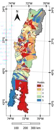
Figure 2.
Map showing the allocation of the most precise model per pixel, represented by (1) PLS-kriging (opt); (2) PLS-kriging (5); (3) Ordinary Kriging; (4) Random Forest-Kriging (5); and, (5) Random Forest-Kriging (opt). Grey colour represents areas with no information.
3.3. Validation of the Models
All of the created models were fitted to the validation dataset and the model statistics are displayed for the top five models (Table 4) and all models (Appendix C). The model ensemble was the least biased (mean bias = −0.0227 m) with the highest precision (RMSE = 1.8505 m, r = 0.8103 and IOA = 0.7228). The five models that were used in order to create the ensemble were also the next most precise, with RMSE ranging from 1.8888–2.0373 m (Table 4) and mean bias ranging from 0.0309–0.5537 m. The number of variables included in the model did not markedly affect model precision, as these five models included regression kriged PLS and RF models that had either five variables or the entire set of covariates (18 for PLS and 20 for RF).
Table 4.
Model validation for different statistical estimators showing mean bias (MB), root mean square error (RMSE), Pearson correlation coefficient (r), and Index of Agreement based on Willmontt (IOA). The term “opt” or “5” is added to specify if the model uses the top five or the optimum number of covariates.
A plot of predicted against actual and residual values for the ensemble showed little apparent bias (Figure 3). This bias was smallest for the high density observations and residuals for these observations largely did not exceed 2 m. However the model did slightly overpredict at low values and underpredict at high values of Site Index, but this bias was generally constrained to outlying points that occurred at low density (Figure 3).
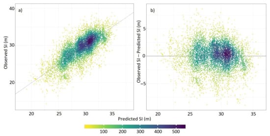
Figure 3.
Relationship between Site Index predicted by the ensemble model and (a) observed Site Index and (b) residual Site Index.
3.4. Predictions of the Models
Figure 4 illustrates the SI prediction of the five most precise models along with the ensemble approach. All five models that were used to produce the ensemble show the highest values of Site Index occurred at a latitude of ca. 36–38 S within coastal and some parts of the inland areas. With the exception of OK, the lowest Site Index was predicted to occur in northern regions and in eastern regions that are close to the Andes. OK did not predict low values in eastern regions, as there were few plots in this area, but did predict low values in the north, where the plot density was higher. Predictions from the ensemble largely reflected the values from the five constituent models. This model predicted moderate to high values of Site Index in coastal areas and within the central valley with the lowest predicted values occurring in the eastern and northern regions.
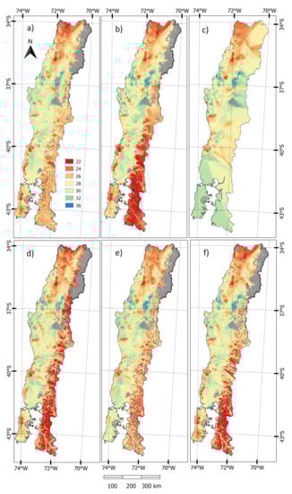
Figure 4.
Site Index predictions from the five most precise models and the ensemble approach; (a) Random Forest-Kriging(opt); (b) Random Forest-Kriging(5); (c) Ordinary Kriging; (d) PLS-Kriging(opt); (e) PLS-Kriging(5); and, (f) Ensemble map. Areas that are coloured grey are regions with no information.
4. Discussion
This study clearly demonstrated the utility of geostatistical methods for predicting the Site Index of P. radiata. While using a novel spatial ensemble approach, the most precise model for each pixel was combined in order to produce an overall model with a more precise prediction that the constituent models. The final model had an RMSE of 1.88 m which compared favourably with previous predictions for both P. radiata and other coniferous species [3,19,33,34]. The variable reduction process highlighted the sensitivity of Site Index to climatic and edaphic factors.
The geostatistical models of ordinary kriging or regression kriging provided the most precise predictions of Site Index among the compared methods. Previous studies have primarily focused on comparisons of precision between the models of Site Index, which do not include a geostatistical component, demonstrating that non-parametric generally outperform parametric models [33,45,46]. Our results extend this research through demonstrating that the addition of a spatial component to both of these model types outperforms models without this component. Gains through regression kriging over the base model were particularly marked for the most precise model, which utilised PLS (r = 0.807 vs 0.705), demonstrating the utility of this approach. Although regression kriging has been widely used for prediction in other domains [67,77,78], with few exceptions very little research has used regression kriging for prediction of productivity indices. As noted by Samuel-Rosa et al. [79], there was generally a consistent but small reduction in precision when the number of variables in the models was reduced from between 18–20 to five.
Regression kriging and ordinary kriging have been found to be the most precise when applied to high density datasets. The accuracy of OK is most influenced by the spatial point pattern (random, aggregated, or regular), sampling density (high or low), autocorrelation, data distribution (normal and skewed), and heterogeneity of the data [80]. The high density of observations in this study favoured the use of ordinary kriging and regression kriging, which is consistent with a model of P. radiata Site Index developed in New Zealand [19]. Regression kriging is less sensitive to the spatial distribution of the sample plots than ordinary kriging, as this method also includes an underlying model that is based on environmental variables. As a result, regression kriging can outperform OK when datasets include a range of plot densities across the area of interest (e.g., [19]).
A novel ensemble approach was used here to spatially combine predictions from the five most precise prediction models. Although ensemble methods have been widely used in other disciplines [52,54,81,82], this method has not previously been used in order to predict Site Index. Most ensemble approaches combine predictions from all models across the entire study area using a range of approaches to weight the individual model predictions [81,83]. Our approach differs in that a single model was used in order to predict Site Index within each pixel, which improved the overall predictive precision over any of the five constituent models.
One of the advantages of our ensemble approach is that this method highlighted regions in which each model performed best, which may be useful if predictions need to be made within a sub-set of the study area. The RF–Kriging method was found to be well suited to northern regions with sparse observations and southern parts of the study area without observations, which highlights the utility of this approach, where the observation density is low. OK had less error in regions where there were both sparse and denser observations. In high altitude eastern areas where the OK model was not selected predictions from this model are likely be higher than actual values as there were not any points to interpolate within this region. In the central part of the study area, as well as southern parts of the Andes, PLS–riging had the lowest prediction error and this region generally included a dense concentration of observations.
The five environmental variables that were the most important determinants of Site Index were all climatic variables for the RF-Kriging model and almost all edaphic variables for the PLS-Kriging model. Growing degree days, accumulated rainfall during years 1 and 4, and variables describing the rainfall and temperature seasonality were the most important climatic determinants of Site Index. Growing degree days has a sound physiological basis as a predictive variable, as P. radiata height extension is strongly regulated by air temperature [84,85] and, consequently, this variable controls the length of the growing season. The sensitivity of Site Index to rainfall has been well established [4,8] and our study clearly demonstrates the importance of adequate rainfall during the years immediately after establishment. The seasonality of air temperature and rainfall were also important regulators of Site Index within Chile, where both of the variables exhibit a marked seasonal variance [86].
Important soil properties included C:N ratio, soil hydraulic conductivity, available soil water, and soil depth. Soil C:N ratio has been found to be a key determinant of conifer productivity [87] and it is a more precise proxy of soil nutrient availability than N as C:N ratio accounts for the positive relationship between carbon content and nitrogen immobilisation [88,89,90,91,92]. Both available soil water and soil depth control the amount of water available to trees which are key attributes within the study area where rainfall is often sparse and highly seasonal [86]. Similarly, soil hydraulic conductivity is also related to water availability and it reflects the soil’s ability to transmit water when subjected to a hydraulic gradient, therefore controlling the partitioning of precipitation between surface runoff and groundwater recharge [93].
Although enhanced vegetation index was not included in the top five variables, variables describing the mean and dispersion of EVI consistently featured among the optimum variables for both types of model. Previous research has found EVI to be a useful predictor of forest canopy structure [94]. There is a strong physiological link between this variable and growth rate, as EVI has also been found to be strongly related to leaf area index (LAI) [95,96] and EVI can also be used in order to identify the start of the growing season [97].
Topographic variables that were well represented for prediction of Site Index in both types of models included terrain surface convexity (TSC) and valley depth. These covariates influence local microclimate and soil-forming processes, and they are consequently associated with the soil type [43]. Both TSC and valley depth are also associated with multiple environmental variables, such as water drainage and water availability, as well as the accumulation of clay and other soil particles. Valley depth is also likely to be a proxy for local exposure to the wind. As higher windspeeds result in reduced tree height and increased diameter [98,99,100,101] P. radiata located in deep valleys with little wind exposure has been found to have significantly greater height than trees that are located on ridges or more exposed areas [102,103].
The direct estimation of Site Index from height data that were collected at the index age of 20 years reduced the error from extrapolation. According to Burkhart and Tomé [104], estimates of Site Index using measurements that coincide with 20 years are rare. As a result, most SI studies use equations to extrapolate height to the required index age, which is an approach that is potentially biased [105,106]. More recent methods, such as the generalised algebraic difference approach (GADA), which include polymorphic models, provide a more accurate estimation method, but still include uncertainties in the final prediction [105]. An additional advantage of using an older dataset was that site specific climatic conditions could be estimated over a uniform period of the rotation length from establishment to 20 years of age.
5. Conclusions
In conclusion, we found geostatistical models of Site Index to outperform a range of parametric and non-parametric models without a geo-spatial component. These five geostatistical models were successfully combined into an ensemble model that was more precise than the constituent models. Climatic and edaphic variables were most strongly related to Site Index, although EVI and many topographic variables were also widely used within the five most precise models. Variables that are related to soil water balance, such as rainfall, soil depth, and water holding capacity, were well represented in the top five models reflecting the importance of water limitations in regulating growth across the study area.
This research highlights the potential improvements that can be gained through the application of sophisticated modelling methods to site productivity modelling, which are likely to be transferrable to other species and countries. Although geostatistical models, such as Ordinary Kriging, are not likely to be as applicable in situations with sparser datasets the regression models used here would be applicable under these circumstances. Future research should more fully utilise LiDAR from existing plantations, as these data can be used to estimate height and Site Index very precisely. In the context of this study, LiDAR can also be used as a supplemental form of plot data, which could prove to be useful when existing plot data are sparse or do not completely cover all environmental conditions. These estimates can be used as input to machine learning and geostatistical models to generate surfaces and predictions of Site Index for unplanted sites.
Author Contributions
Conceptualization, G.G.-A. and G.F.O.; Data curation, P.M.-Q.; Formal analysis, G.G.-A., G.F.O. and M.S.W.; Funding acquisition, B.B.-K.; Methodology, G.G.-A., G.F.O., P.M.-Q., M.G. and M.S.W.; Validation, M.S.W.; Visualization, B.B.-K.; Writing—Original draft, G.G.-A., G.F.O. and M.S.W.; Writing—Review & editing, P.M.-Q., M.G., B.B.-K. and M.S.W. All authors have read and agreed to the published version of the manuscript.
Funding
This research received no external funding.
Institutional Review Board Statement
Not applicable.
Informed Consent Statement
Not applicable.
Data Availability Statement
The data presented in this study are available on request from the corresponding author. The data are not publicly available due to privacy.
Acknowledgments
The authors would like to thank Forestal Arauco, for their role in providing the study site observations, and financial support to this study. Additionally, we want to acknowledge Rodrigo Sobarzo, Fernando Bustamante, Juan Jose Rivera and Eldemar Jaskiu from Forestal Arauco for validating and reviewing the content of this document. Special thanks to Rodrigo Ahumada and Sebastian Fernandez for their support in the publication of this manuscript.
Conflicts of Interest
The authors declare no conflict of interest.
Appendix A
Appendix A.1. Parametric Models
Appendix A.1.1. Multiple Linear Regression
Multiple linear regression is a statistical method that predicts the response variable from more than one independent variable. Use of this method assumes that independent variables are not too highly correlated and that residuals from the final model are normally distributed [107].
Appendix A.1.2. Partial Least Squares
Partial least squares (PLS) condenses the most useful information from a large number of predictors to a reduced set of uncorrelated components. These components are then used within a regression to predict the dependant variable [3,108]. The main advantage of this method is that provides a lower risk of chance correlation and higher predictive accuracy than multiple regression particularly when there are a large number of correlated predictors in the dataset [109]. The number of components within the model was optimised.
Appendix A.1.3. Elastic Net
Elastic net (EN) is a form of regularised regression. This method incorporates penalities from both lasso and ridge regression that constrain the coefficient size within the model. EN performs automatic variable selection like Lasso, while the penalization from the Ridge term stabilizes the solution paths which improves the prediction accuracy. The model was fitted using the ‘glmnet’ method, which was used to optimise the two hyperparameters alpha (mixing percentage) and lambda (regularization parameter).
Appendix A.2. Non-Parametric Models
Appendix A.2.1. Random Forest
Random Forest (RF) consists of a combination of many binary decision trees built using several bootstrap samples from a supervised machine learning algorithm, which randomly chooses, at each node, a subset of explanatory variables [110]. RF belongs to the family of ensemble methods, in where the final prediction comprises the average predictions from individual trees [111].
Using the caret package [60], a more memory efficient implementation of RF, using the ‘ranger’ method was applied [112]. For this methodology the following parameters were optimised: (i) the number of randomly selected predictors (mtry), (ii) the minimum node size and (iii) the splitting rule.
Appendix A.2.2. Support Vector Machines
Support vector machine (SVM) applies a simple linear technique to the data but in a high-dimensional feature space that is non-linearly related to the input space [113]. The regularized SVM Machine (dual) with Linear Kernel was fitted to the data [60]. The covariates were standardized by pre-processing the predictor data (“center”, and “scale”). The loss function and cost parameters were optimised within the model.
Appendix A.2.3. Neural Network
Neural networks or artificial neural networks (ANN) consist of processing units called neurons or nodes, whose functionality is loosely based on the structure and behaviour of the natural neuron. This technique uses mathematical models that learn nonlinear relationship between the data set, and response variable for both prediction and classification [114]. ANN was fitted using “nnet” method [60] and the hidden units and weight decay parameters were optimised.
Appendix A.2.4. Xgboost
The method eXtreme Gradient Boosting (XGBoost) is a scalable implementation of gradient boosting framework developed by Friedman [115]. XGBoost is a supervised machine learning, using decision-tree algorithms. This method builds models from adding individual so called “weak learners” from a gradient descent algorithm over an objective function. XGBoost used the caret package with the “xgbTree” methodology [60]. The hyperparameters that were tuned for this method, included: (i) boosting iterations, (ii) maximum tree depth, (iii) shrinkage, (iv) minimum loss reduction, (v) subsample ratio of columns, (vi) minimum sum of instance weight, and (vii) subsample percentage.
Appendix A.2.5. Multivariate Adaptive Regression Splines
Multivariate Adaptive Regression Splines (MARS) is a regression technique that captures the nonlinear relationships in the data by assessing cutpoints (knots), which identifies regions where the relationship between the predictor variable and the response changes [116]. The main advantage of MARS is that it enhances the interpretability of complex interactions between the predictor and the response variables. This model was fitted using the “earth” method in the caret package [60], which tuned the number of terms (the maximum number of knots) and the number of variable interactions.
Appendix B
Table A1.
Environmental raster covariates list.
Table A1.
Environmental raster covariates list.
| Code | Category | Description |
|---|---|---|
| AGDD5 | Climate | Growing degrees day base 5 (C) |
| AGDD10 | Climate | Growing degrees day base 10 (C) |
| AGDD15 | Climate | Growing degrees day base 15 (C) |
| Rain | Climate | accumulative rainfall per stand (mm) |
| DH | Climate | accumulative water deficit index per stand (mm) |
| DH4 | Climate | accumulative water deficit index per stand first 4 years (mm) |
| ET | Climate | accumulative evapotranspiration per stand (mm) |
| Rain1 | Climate | accumulative rainfall per stand first year (mm) |
| Rain2 | Climate | accumulative rainfall per stand first 2 years (mm) |
| Rain4 | Climate | accumulative rainfall per stand first 4 years (mm) |
| ColdD | Climate | accumulative cold days per stand (days) |
| biovar.1 | Climate | bio1 = Mean annual temperature (C) |
| biovar.2 | Climate | bio2 = Mean diurnal range (mean of max temp - min temp) (C) |
| biovar.3 | Climate | bio3 = Isothermality (bio2/bio7) (× 100) (%) |
| biovar.4 | Climate | bio4 = Temperature seasonality (standard deviation × 100) (%) |
| biovar.5 | Climate | bio5 = Max temperature of warmest month (C) |
| biovar.6 | Climate | bio6 = Min temperature of coldest month (C) |
| biovar.7 | Climate | bio7 = Temperature annual range (bio5-bio6) (C) |
| biovar.8 | Climate | bio8 = Mean temperature of the wettest quarter (C) |
| biovar.9 | Climate | bio9 = Mean temperature of driest quarter (C) |
| biovar.10 | Climate | bio10 = Mean temperature of warmest quarter (C) |
| biovar.11 | Climate | bio11 = Mean temperature of coldest quarter (C) |
| biovar.12 | Climate | bio12 = Total (annual) precipitation (mm) |
| biovar.13 | Climate | bio13 = Precipitation of wettest month (mm) |
| biovar.14 | Climate | bio14 = Precipitation of driest month (mm) |
| biovar.15 | Climate | bio15 = Precipitation seasonality (coefficient of variation) (%) |
| biovar.16 | Climate | bio16 = Precipitation of wettest quarter (mm) |
| biovar.17 | Climate | bio17 = Precipitation of driest quarter (mm) |
| biovar.18 | Climate | bio18 = Precipitation of warmest quarter (mm) |
| biovar.19 | Climate | bio19= Precipitation of coldest quarter (mm) |
| Frost | Climate | average number of cold Day (days) |
| PRM | Soil Morphology | Parent rock material |
| BLD | Soil Properties | Bulk density |
| SHC_0_30 | Soil Properties | Soil hydraulic conductivity (0–30 cm) |
| CLAY | Soil Properties | Clay content (%) |
| ASW | Soil Properties | Available soil water |
| N_0_60 | Soil Properties | Total Nitrogen content from 0 to 60 cm of soil depth (kg/ha) |
| C_N | Soil Properties | Carbon to Nitrogen ratio |
| SoilDepth | Soil Properties | Soil Depth |
| Elevation | Topography | LiDAR + SRTM elevation (m.a.s.l) |
| Aspect | Topography | Aspect Degree (%) |
| Slope | Topography | Slope Degree (%) |
| CNBL | Topography | Channel Network Base Level (m.a.s.l) |
| CND | Topography | Channel Network Distance |
| LC | Topography | Longitudinal Curvature |
| CI | Topography | Convergence Index |
| LS_factor | Topography | Slope Length and Steepness Factor |
| Max_Curv | Topography | Maximal Curvature |
| Min_Curv | Topography | Minimal Curvature |
| Prof_Curv | Topography | Profile Curvature |
| Tang_Curv | Topography | Tangential Curvature |
| TSC | Topography | Terrain Surface Convexity |
| TRI | Topography | Terrain ruggedness index |
| TPI | Topography | Topographic Position Index |
| TWI | Topography | Topographic Wetness Index |
| ValDepth | Topography | Valley Depth |
| EVI_mean | Vegetation | Average Enhance vegetation index from last 20 years |
| EVI_min | Vegetation | Minimum Enhance vegetation index from last 20 years |
| EVI_peak | Vegetation | Maximum Enhance vegetation index from last 20 years |
| EVI_range | Vegetation | Enhanced vegetation index range from last 20 years |
| EVI_sd | Vegetation | Standard deviation for EVI from last 20 years |
| PWU | Water balance | Potential water use |
| WDI | Water balance | Water deficit index |
| WS | Water balance | Water surplus |
Appendix C
Spatial model validation, including the ensemble approach with the validation data set.
Table A2.
Model validation to different statistical estimators. Mean Bias (MB), Root mean square error (RMSE), Pearson correlation coefficient (r) and Index of Agreement based on Willmontt (IOA). The term “opt” or “5” is added to specify if the model use the top five or the optimum number of covariates.
| Model | MB | RMSE | R | IOA |
|---|---|---|---|---|
| Model Ensemble | −0.0228 | 1.8505 | 0.8103 | 0.7229 |
| PLS-kriging(opt) | 0.2609 | 1.8884 | 0.8074 | 0.7154 |
| Ordinary Kriging | 0.1813 | 1.9477 | 0.7888 | 0.7059 |
| PLS-kriging(5) | 0.0368 | 1.9587 | 0.7901 | 0.7009 |
| Random Forest-Kriging(5) | 0.1767 | 1.9927 | 0.7849 | 0.7035 |
| Random Forest-Kriging(opt) | 0.5590 | 2.0340 | 0.7864 | 0.6921 |
| Random Forest (opt) | 0.5334 | 2.0496 | 0.7793 | 0.6844 |
| XGBoost (opt) | 0.5996 | 2.1420 | 0.7583 | 0.6714 |
| Random Forest(5) | 0.6542 | 2.1795 | 0.7521 | 0.6708 |
| Neural network(opt) | 0.2924 | 2.3034 | 0.7010 | 0.6524 |
| XGBoost(5) | 0.8710 | 2.3129 | 0.7344 | 0.6354 |
| MARS(opt) | 0.6446 | 2.4419 | 0.6934 | 0.6106 |
| PLS(opt) | 1.2366 | 2.5921 | 0.7052 | 0.5924 |
| Multiple linear regression(opt) | 1.2368 | 2.5922 | 0.7052 | 0.5924 |
| Elastic net(opt) | 1.2429 | 2.6019 | 0.7030 | 0.5907 |
| Neural network(5) | 1.0331 | 2.6561 | 0.6380 | 0.5924 |
| MARS(5) | 1.6199 | 2.8209 | 0.6929 | 0.5499 |
| Support vector machine(opt) | 1.1034 | 3.1136 | 0.4028 | 0.5114 |
| Multiple linear regression(5) | 1.7278 | 3.3910 | 0.4025 | 0.4514 |
| PLS(5) | 1.7298 | 3.3930 | 0.4036 | 0.4513 |
| Support vector machine(5) | 3.1245 | 4.5882 | −0.1750 | 0.2521 |
| Elastic net(5) | 20.3880 | 20.9859 | 0.2763 | −0.7439 |
References
- Salas, C.; Donoso, P.J.; Vargas, R.; Arriagada, C.A.; Pedraza, R.; Soto, D.P. The Forest Sector in Chile: An Overview and Current Challenges. J. For. 2016, 114, 562–571. [Google Scholar] [CrossRef]
- Lewis, N.B.; Ferguson, I.S.; Sutton, W.; Donald, D.; Lisboa, H. Management of Radiata Pine; Inkata Press Pty Ltd/Butterworth-Heinemann: New South Wales, Australia, 1993. [Google Scholar]
- Palmer, D.J.; Höck, B.; Kimberley, M.O.; Watt, M.S.; Lowe, D.J.; Payn, T.W. Comparison of spatial prediction techniques for developing Pinus radiata productivity surfaces across New Zealand. For. Ecol. Manag. 2009, 258, 2046–2055. [Google Scholar] [CrossRef]
- Watt, M.S.; Palmer, D.J.; Kimberley, M.O.; Höck, B.K.; Payn, T.W.; Lowe, D.J. Development of models to predict Pinus radiata productivity throughout New Zealand. Can. J. For. Res. 2010, 40, 488–499. [Google Scholar] [CrossRef]
- Landsberg, J.; Waring, R. A generalised model of forest productivity using simplified concepts of radiation-use efficiency, carbon balance and partitioning. For. Ecol. Manag. 1997, 95, 209–228. [Google Scholar] [CrossRef]
- Kirschbaum, M.U. CenW, a forest growth model with linked carbon, energy, nutrient and water cycles. Ecol. Model. 1999, 118, 17–59. [Google Scholar] [CrossRef]
- Battaglia, M.; Sands, P.; White, D.; Mummery, D. CABALA: A linked carbon, water and nitrogen model of forest growth for silvicultural decision support. For. Ecol. Manag. 2004, 193, 251–282. [Google Scholar] [CrossRef]
- Kirschbaum, M.U.; Watt, M.S. Use of a process-based model to describe spatial variation in Pinus radiata productivity in New Zealand. For. Ecol. Manag. 2011, 262, 1008–1019. [Google Scholar] [CrossRef]
- Pinjuv, G.; Mason, E.G.; Watt, M. Quantitative validation and comparison of a range of forest growth model types. For. Ecol. Manag. 2006, 236, 37–46. [Google Scholar] [CrossRef]
- Garcia, O. A stochastic differential equation model for the height growth of forest stands. Biometrics 1983, 39, 1059–1072. [Google Scholar] [CrossRef]
- Clutter, J.L.; Fortson, J.C.; Pienaar, L.V.; Brister, G.H.; Bailey, R.L. Timber Management: A Quantitative Approach; John Wiley & Sons, Inc.: New York, NY, USA, 1983. [Google Scholar]
- García, O. Height growth of Pinus radiata in New Zealand. N. Z. J. For. Sci. 1999, 29, 131–145. [Google Scholar]
- Skovsgaard, J.P.; Vanclay, J.K. Forest site productivity: A review of the evolution of dendrometric concepts for even-aged stands. Forestry 2008, 81, 13–31. [Google Scholar] [CrossRef]
- Bontemps, J.D.; Bouriaud, O. Predictive approaches to forest site productivity: Recent trends, challenges and future perspectives. Forestry 2014, 87, 109–128. [Google Scholar] [CrossRef]
- Eichhorn, F. Beziehungen zwischen bestandshöhe und bestandsmasse. Allgemeine Forst und Jagdzeitung 1904, 80, 45–49. [Google Scholar]
- Lanner, R.M. On the insensitivity of height growth to spacing. For. Ecol. Manag. 1985, 13, 143–148. [Google Scholar] [CrossRef]
- Maclaren, J.; Grace, J.; Kimberley, M.; Knowles, R.; West, G. Height growth of Pinus radiata as affected by stocking. N. Z. J. For. Sci 1995, 25, 73–90. [Google Scholar]
- Pienaar, L.V.; Shiver, B.D. The effect of planting density on dominant height in unthinned slash pine plantations. For. Sci. 1984, 30, 1059–1066. [Google Scholar]
- Kimberley, M.O.; Watt, M.S.; Harrison, D. Characterising prediction error as a function of scale in spatial surfaces of tree productivity. N. Z. J. For. Sci. 2017, 47, 1–11. [Google Scholar] [CrossRef]
- Fontes, L.; Tomé, M.; Thompson, F.; Yeomans, A.; Luis, J.S.; Savill, P. Modelling the Douglas-fir (Pseudotsuga menziesii (Mirb.) Franco) site index from site factors in Portugal. Forestry 2003, 76, 491–507. [Google Scholar] [CrossRef]
- Monserud, R.A.; Huang, S.; Yang, Y. Predicting lodgepole pine site index from climatic parameters in Alberta. For. Chron. 2006, 82, 562–571. [Google Scholar] [CrossRef]
- Palmer, D.J.; Watt, M.S.; Kimberley, M.O.; Dungey, H.S. Predicting the spatial distribution of Sequoia sempervirens productivity in New Zealand. N. Z. J. For. Sci. 2012, 42, 81–89. [Google Scholar]
- Seynave, I.; Gégout, J.C.; Hervé, J.C.; Dhôte, J.F.; Drapier, J.; Bruno, É.; Dumé, G. Picea abies site index prediction by environmental factors and understorey vegetation: A two-scale approach based on survey databases. Can. J. For. Res. 2005, 35, 1669–1678. [Google Scholar] [CrossRef]
- Wang, G.G.; Huang, S.; Monserud, R.A.; Klos, R.J. Lodgepole pine site index in relation to synoptic measures of climate, soil moisture and soil nutrients. For. Chron. 2004, 80, 678–686. [Google Scholar] [CrossRef]
- Watt, M.S.; Palmer, D.J.; Dungey, H.; Kimberley, M.O. Predicting the spatial distribution of Cupressus lusitanica productivity in New Zealand. For. Ecol. Manag. 2009, 258, 217–223. [Google Scholar] [CrossRef]
- Watt, M.S.; Dash, J.P.; Bhandari, S.; Watt, P. Comparing parametric and non-parametric methods of predicting Site Index for radiata pine using combinations of data derived from environmental surfaces, satellite imagery and airborne laser scanning. For. Ecol. Manag. 2015, 357, 1–9. [Google Scholar] [CrossRef]
- Kimberley, M.; West, G.; Dean, M.; Knowles, L. The 300 Index-a volume productivity index for radiata pine. N. Z. J. For. 2005, 50, 13–18. [Google Scholar]
- Perron, J. Inventaire forestier. In Manuel de Foresterie; Les Presses de l’Université Laval: Sainte-Foy, QC, Canada, 1996; pp. 390–473. [Google Scholar]
- McLeod, S.D.; Running, S.W. Comparing site quality indices and productivity in ponderosa pine stands of western Montana. Can. J. For. Res. 1988, 18, 346–352. [Google Scholar] [CrossRef]
- Duncker, P.S.; Barreiro, S.M.; Hengeveld, G.M.; Lind, T.; Mason, W.L.; Ambrozy, S.; Spiecker, H. Classification of forest management approaches: A new conceptual framework and its applicability to European forestry. Ecol. Soc. 2012, 17. [Google Scholar] [CrossRef]
- Arano, K.G.; Munn, I.A. Evaluating forest management intensity: A comparison among major forest landowner types. For. Policy Econ. 2006, 9, 237–248. [Google Scholar] [CrossRef]
- Watt, M.S.; Kimberley, M.O.; Dash, J.P.; Harrison, D. Spatial prediction of optimal final stand density for even-aged plantation forests using productivity indices. Can. J. For. Res. 2017, 47, 527–535. [Google Scholar] [CrossRef]
- Aertsen, W.; Kint, V.; Van Orshoven, J.; Muys, B. Evaluation of modelling techniques for forest site productivity prediction in contrasting ecoregions using stochastic multicriteria acceptability analysis (SMAA). Environ. Model. Softw. 2011, 26, 929–937. [Google Scholar] [CrossRef]
- Aertsen, W.; Kint, V.; Van Orshoven, J.; Özkan, K.; Muys, B. Comparison and ranking of different modelling techniques for prediction of site index in Mediterranean mountain forests. Ecol. Model. 2010, 221, 1119–1130. [Google Scholar] [CrossRef]
- Chen, H.Y.; Krestov, P.V.; Klinka, K. Trembling aspen site index in relation to environmental measures of site quality at two spatial scales. Can. J. For. Res. 2002, 32, 112–119. [Google Scholar] [CrossRef]
- Codilan, A.L.; Nakajima, T.; Tatsuhara, S.; Shiraishi, N. Estimating site index from ecological factors for industrial tree plantation species in Mindanao, Philippines. Bull. Univ. Tokyo For. 2015, 133, 19–41. [Google Scholar]
- Hamel, B.; Bélanger, N.; Paré, D. Productivity of black spruce and Jack pine stands in Quebec as related to climate, site biological features and soil properties. For. Ecol. Manag. 2004, 191, 239–251. [Google Scholar] [CrossRef]
- Nigh, G.D.; Ying, C.C.; Qian, H. Climate and productivity of major conifer species in the interior of British Columbia, Canada. For. Sci. 2004, 50, 659–671. [Google Scholar]
- Pinno, B.D.; Paré, D.; Guindon, L.; Bélanger, N. Predicting productivity of trembling aspen in the Boreal Shield ecozone of Quebec using different sources of soil and site information. For. Ecol. Manag. 2009, 257, 782–789. [Google Scholar] [CrossRef]
- Sánchez-Rodrıguez, F.; Rodrıguez-Soalleiro, R.; Español, E.; López, C.; Merino, A. Influence of edaphic factors and tree nutritive status on the productivity of Pinus radiata D. Don plantations in northwestern Spain. For. Ecol. Manag. 2002, 171, 181–189. [Google Scholar] [CrossRef]
- Seynave, I.; Gégout, J.C.; Hervé, J.C.; Dhôte, J.F. Is the spatial distribution of European beech (Fagus sylvatica L.) limited by its potential height growth? J. Biogeogr. 2008, 35, 1851–1862. [Google Scholar] [CrossRef]
- Sharma, R.P.; Brunner, A.; Eid, T. Site index prediction from site and climate variables for Norway spruce and Scots pine in Norway. Scand. J. For. Res. 2012, 27, 619–636. [Google Scholar] [CrossRef]
- Socha, J. Effect of topography and geology on the site index of Picea abies in the West Carpathian, Poland. Scand. J. For. Res. 2008, 23, 203–213. [Google Scholar] [CrossRef]
- Wang, G.G. White spruce site index in relation to soil, understory vegetation, and foliar nutrients. Can. J. For. Res. 1995, 25, 29–38. [Google Scholar] [CrossRef]
- González-Rodríguez, M.A.; Diéguez-Aranda, U. Exploring the use of learning techniques for relating the site index of radiata pine stands with climate, soil and physiography. For. Ecol. Manag. 2020, 458, 117803. [Google Scholar] [CrossRef]
- Sabatia, C.O.; Burkhart, H.E. Predicting site index of plantation loblolly pine from biophysical variables. For. Ecol. Manag. 2014, 326, 142–156. [Google Scholar] [CrossRef]
- Weiskittel, A.R.; Crookston, N.L.; Radtke, P.J. Linking climate, gross primary productivity, and site index across forests of the western United States. Can. J. For. Res. 2011, 41, 1710–1721. [Google Scholar] [CrossRef]
- Shen, C.; Lei, X.; Liu, H.; Wang, L.; Liang, W. Potential impacts of regional climate change on site productivity of Larix olgensis plantations in northeast China. iForest Biogeosci. For. 2015, 8, 642. [Google Scholar] [CrossRef]
- Cutler, D.R.; Edwards, T.C., Jr.; Beard, K.H.; Cutler, A.; Hess, K.T.; Gibson, J.; Lawler, J.J. Random forests for classification in ecology. Ecology 2007, 88, 2783–2792. [Google Scholar] [CrossRef]
- Drake, J.M.; Randin, C.; Guisan, A. Modelling ecological niches with support vector machines. J. Appl. Ecol. 2006, 43, 424–432. [Google Scholar] [CrossRef]
- Górecki, T.; Krzyśko, M. Regression methods for combining multiple classifiers. Commun. Stat. Simul. Comput. 2015, 44, 739–755. [Google Scholar] [CrossRef]
- Taghizadeh-Mehrjardi, R.; Minasny, B.; Toomanian, N.; Zeraatpisheh, M.; Amirian-Chakan, A.; Triantafilis, J. Digital Mapping of Soil Classes Using Ensemble of Models in Isfahan Region, Iran. Soil Syst. 2019, 3, 37. [Google Scholar] [CrossRef]
- Swiderski, B.; Osowski, S.; Kruk, M.; Barhoumi, W. Aggregation of classifiers ensemble using local discriminatory power and quantiles. Expert Syst. Appl. 2016, 46, 316–323. [Google Scholar] [CrossRef]
- Dobarco, M.R.; Arrouays, D.; Lagacherie, P.; Ciampalini, R.; Saby, N.P. Prediction of topsoil texture for Region Centre (France) applying model ensemble methods. Geoderma 2017, 298, 67–77. [Google Scholar] [CrossRef]
- García, O. Indices de Sitio Para Pino Insigne en Chile: Instituto Forestal; Serie de Investigacion, Number 2 in January 1970; Instituto Forestal: Santiago, Chile, 1970; p. 30. [Google Scholar]
- Goulding, C. Measurement of trees. In Forestry Handbook; The New Zealand Institute of Forestry (Inc.): Christchurch, New Zealand, 2005; Volume 2005, pp. 145–148. [Google Scholar]
- Palmer, D.J.; Kimberley, M.O.; Cown, D.J.; McKinley, R.B. Assessing prediction accuracy in a regression kriging surface of Pinus radiata outerwood density across New Zealand. For. Ecol. Manag. 2013, 308, 9–16. [Google Scholar] [CrossRef]
- De Visualización, P.L.P. Guía de Referencia para la Plataforma de Visualización de Simulaciones Climáticas. Available online: https://http://www.cr2.cl/guia-de-referencia-para-la-plataforma-de-visualizacion-de-simulaciones-climaticas-cr2/ (accessed on 1 May 2020).
- Weston, J.; Elisseeff, A.; Schölkopf, B.; Tipping, M. Use of the zero-norm with linear models and kernel methods. J. Mach. Learn. Res. 2003, 3, 1439–1461. [Google Scholar]
- Kuhn, M. The Caret Package; R Foundation for Statistical Computing: Vienna, Austria, 2012. [Google Scholar]
- Chen, X.w.; Jeong, J.C. Enhanced recursive feature elimination. In Proceedings of the Sixth International Conference on Machine Learning and Applications (ICMLA 2007), Cincinnati, OH, USA, 13–15 December 2007; pp. 429–435. [Google Scholar]
- Guyon, I.; Weston, J.; Barnhill, S.; Vapnik, V. Gene selection for cancer classification using support vector machines. Mach. Learn. 2002, 46, 389–422. [Google Scholar] [CrossRef]
- Bahl, A.; Hellack, B.; Balas, M.; Dinischiotu, A.; Wiemann, M.; Brinkmann, J.; Luch, A.; Renard, B.Y.; Haase, A. Recursive feature elimination in random forest classification supports nanomaterial grouping. NanoImpact 2019, 15, 100179. [Google Scholar] [CrossRef]
- Bruce, P.; Bruce, A. Practical Statistics for Data Scientists: 50 Essential Concepts; O’Reilly Media, Inc.: Sebastopol, CA, USA, 2017. [Google Scholar]
- Tibshirani, R. Regression shrinkage and selection via the lasso. J. R. Stat. Soc. Ser. (Methodol.) 1996, 58, 267–288. [Google Scholar] [CrossRef]
- Akinwande, M.O.; Dikko, H.G.; Samson, A. Variance inflation factor: As a condition for the inclusion of suppressor variable (s) in regression analysis. Open J. Stat. 2015, 5, 754. [Google Scholar] [CrossRef]
- Hengl, T.; Nussbaum, M.; Wright, M.N.; Heuvelink, G.B.; Gräler, B. Random forest as a generic framework for predictive modeling of spatial and spatio-temporal variables. PeerJ 2018, 6, e5518. [Google Scholar] [CrossRef]
- Pham, T.D.; Yokoya, N.; Xia, J.; Ha, N.T.; Le, N.N.; Nguyen, T.T.T.; Dao, T.H.; Vu, T.T.P.; Pham, T.D.; Takeuchi, W. Comparison of Machine Learning Methods for Estimating Mangrove Above-Ground Biomass Using Multiple Source Remote Sensing Data in the Red River Delta Biosphere Reserve, Vietnam. Remote Sens. 2020, 12, 1334. [Google Scholar] [CrossRef]
- Olmedo, G.F.; Guevara, M.; Gavilan, G. Code for Building Pixel by Pixel Spatial Ensemble of Machine Learning Models. Zenodo 2020. [Google Scholar] [CrossRef]
- Hengl, T.; Heuvelink, G.B.; Rossiter, D.G. About regression-kriging: From equations to case studies. Comput. Geosci. 2007, 33, 1301–1315. [Google Scholar] [CrossRef]
- Guevara, M.A.; Olmedo, G.F. Model evaluation in digital soil mapping. In Soil Organic Carbon Mapping Cookbook, Chapter 8, 2nd ed.; Yigini, Y., Olmedo, G.F., Reiter, S., Baritz, R., Viatkin, K., Vargas, R.R., Eds.; FAO: Rome, Italy, 2018; pp. 133–143. [Google Scholar]
- Farmer, W.H. Ordinary kriging as a tool to estimate historical daily streamflow records. Hydrol. Earth Syst. Sci. 2016, 20, 2721. [Google Scholar] [CrossRef]
- Odeh, I.O.; McBratney, A.; Chittleborough, D. Further results on prediction of soil properties from terrain attributes: Heterotopic cokriging and regression-kriging. Geoderma 1995, 67, 215–226. [Google Scholar] [CrossRef]
- Hengl, T.; Heuvelink, G.B.; Stein, A. A generic framework for spatial prediction of soil variables based on regression-kriging. Geoderma 2004, 120, 75–93. [Google Scholar] [CrossRef]
- Hiemstra, P.; Hiemstra, M.P. Package ‘automap’. Compare 2013, 105, 10. [Google Scholar]
- Carslaw, D.C.; Ropkins, K. Openair—An R package for air quality data analysis. Environ. Model. Softw. 2012, 27, 52–61. [Google Scholar] [CrossRef]
- Fox, E.W.; Ver Hoef, J.M.; Olsen, A.R. Comparing spatial regression to random forests for large environmental data sets. PLoS ONE 2020, 15, e0229509. [Google Scholar] [CrossRef]
- Li, J.; Heap, A.D.; Potter, A.; Huang, Z.; Daniell, J.J. Can we improve the spatial predictions of seabed sediments? A case study of spatial interpolation of mud content across the southwest Australian margin. Cont. Shelf Res. 2011, 31, 1365–1376. [Google Scholar] [CrossRef]
- Samuel-Rosa, A.; Heuvelink, G.; Vasques, G.; Anjos, L. Do more detailed environmental covariates deliver more accurate soil maps? Geoderma 2015, 243, 214–227. [Google Scholar] [CrossRef]
- Eldeiry, A.A.; Garcia, L.A. Evaluating the performance of ordinary kriging in mapping soil salinity. J. Irrig. Drain. Eng. 2012, 138, 1046–1059. [Google Scholar] [CrossRef]
- Diks, C.G.; Vrugt, J.A. Comparison of point forecast accuracy of model averaging methods in hydrologic applications. Stoch. Environ. Res. Risk Assess. 2010, 24, 809–820. [Google Scholar] [CrossRef]
- Padarian, J.; Minasny, B.; McBratney, A.; Dalgliesh, N. Predicting and mapping the soil available water capacity of Australian wheatbelt. Geoderma Reg. 2014, 2, 110–118. [Google Scholar] [CrossRef]
- Nisbet, R.; Elder, J.; Miner, G. Handbook of Statistical Analysis and Data Mining Applications; Academic Press: Oxford, UK, 2009. [Google Scholar]
- Whitehead, D.; Kelliher, F.M.; Frampton, C.M.; Godfrey, M.J. Seasonal development of leaf area in a young, widely spaced Pinus radiata D. Don stand. Tree Physiol. 1994, 14, 1019–1038. [Google Scholar] [CrossRef] [PubMed]
- Kimberley, M.O.; Richardson, B. Importance of seasonal growth patterns in modelling interactions between radiata pine and some common weed species. Can. J. For. Res. 2004, 34, 184–194. [Google Scholar] [CrossRef]
- Watt, M.S.; Trincado, G. Modelling the influence of environment on basic density of the juvenile wood for Pinus radiata grown in Chile. For. Ecol. Manag. 2019, 448, 112–118. [Google Scholar] [CrossRef]
- Watt, M.S.; Davis, M.R.; Clinton, P.W.; Coker, G.; Ross, C.; Dando, J.; Parfitt, R.L.; Simcock, R. Identification of key soil indicators influencing plantation productivity and sustainability across a national trial series in New Zealand. For. Ecol. Manag. 2008, 256, 180–190. [Google Scholar] [CrossRef]
- Goodale, C.L.; Aber, J.D. The long-term effects of land-use history on nitrogen cycling in northern hardwood forests. Ecol. Appl. 2001, 11, 253–267. [Google Scholar] [CrossRef]
- Andersson, P.; Berggren, D.; Nilsson, I. Indices for nitrogen status and nitrate leaching from Norway spruce (Picea abies (L.) Karst.) stands in Sweden. For. Ecol. Manag. 2002, 157, 39–53. [Google Scholar] [CrossRef]
- Ross, D.S.; Lawrence, G.B.; Fredriksen, G. Mineralization and nitrification patterns at eight northeastern USA forested research sites. For. Ecol. Manag. 2004, 188, 317–335. [Google Scholar] [CrossRef]
- Parfitt, R.; Ross, D.; Coomes, D.; Richardson, S.; Smale, M.; Dahlgren, R. N and P in New Zealand soil chronosequences and relationships with foliar N and P. Biogeochemistry 2005, 75, 305–328. [Google Scholar] [CrossRef]
- Parfitt, R.; Yeates, G.; Ross, D.; Mackay, A.; Budding, P. Relationships between soil biota, nitrogen and phosphorus availability, and pasture growth under organic and conventional management. Appl. Soil Ecol. 2005, 28, 1–13. [Google Scholar] [CrossRef]
- Jarvis, N.; Koestel, J.; Messing, I.; Moeys, J.; Lindahl, A. Influence of soil, land use and climatic factors on the hydraulic conductivity of soil. Hydrol. Earth Syst. Sci. Discuss. 2013, 10, 10845–10872. [Google Scholar] [CrossRef]
- Chen, J.; Sun, L. Using MODIS EVI to detect vegetation damage caused by the 2008 ice and snow storms in south China. J. Geophys. Res. Biogeosci. 2010, 115, 1–12. [Google Scholar] [CrossRef]
- Alexandridis, T.K.; Ovakoglou, G.; Clevers, J.G. Relationship between MODIS EVI and LAI across time and space. Geocarto Int. 2019, 35, 1385–1399. [Google Scholar] [CrossRef]
- Potithep, S.; Nagai, S.; Nasahara, K.N.; Muraoka, H.; Suzuki, R. Two separate periods of the LAI–VIs relationships using in situ measurements in a deciduous broadleaf forest. Agric. For. Meteorol. 2013, 169, 148–155. [Google Scholar] [CrossRef]
- Karkauskaite, P.; Tagesson, T.; Fensholt, R. Evaluation of the plant phenology index (PPI), NDVI and EVI for start-of-season trend analysis of the Northern Hemisphere boreal zone. Remote Sens. 2017, 9, 485. [Google Scholar] [CrossRef]
- Jacobs, M. The effect of wind sway on the form and development of Pinus radiata D. Don. Aust. J. Bot. 1954, 2, 35–51. [Google Scholar] [CrossRef]
- Telewski, F.W.; Jaffe, M.J. Thigmomorphogenesis: Anatomical, morphological and mechanical analysis of genetically different sibs of Pinus taeda in response to mechanical perturbation. Physiol. Plant. 1986, 66, 219–226. [Google Scholar] [CrossRef]
- Telewski, F.W.; Jaffe, M.J. Thigmomorphogenesis: Field and laboratory studies of Abies fraseri in response to wind or mechanical perturbation. Physiol. Plant. 1986, 66, 211–218. [Google Scholar] [CrossRef]
- Telewski, F. Structure and function of flexure wood in Abies fraseri. Tree Physiol. 1989, 5, 113–121. [Google Scholar] [CrossRef]
- Watt, M.; Moore, J.; McKinlay, B. The influence of wind on branch characteristics of Pinus radiata. Trees 2005, 19, 58–65. [Google Scholar] [CrossRef]
- Watt, M.S.; Kirschbaum, M.U. Moving beyond simple linear allometric relationships between tree height and diameter. Ecol. Model. 2011, 222, 3910–3916. [Google Scholar] [CrossRef]
- Burkhart, H.E.; Tomé, M. Modeling Forest Trees and Stands; Springer Science & Business Media: Dordrecht, The Netherlands, 2012. [Google Scholar]
- Socha, J.; Pierzchalski, M.; Bałazy, R.; Ciesielski, M. Modelling top height growth and site index using repeated laser scanning data. For. Ecol. Manag. 2017, 406, 307–317. [Google Scholar] [CrossRef]
- Cieszewski, C.J.; Harrison, M.; Martin, S.W. Examples of practical methods for unbiased parameter estimation in self-referencing functions. In Proceedings of the First International Conference on Measurements and Quantitative Methods and Management, Jekyll Island, GA, USA, 17–18 November 1999. [Google Scholar]
- Seal, H.L. The Historical Development of the Gauss Linear Model; Yale University: New Haven, CT, USA, 1968. [Google Scholar]
- Wold, S.; Geladi, P.; Esbensen, K.; Öhman, J. Multi-way principal components-and PLS-analysis. J. Chemom. 1987, 1, 41–56. [Google Scholar] [CrossRef]
- Cramer, R.D. Partial least squares (PLS): Its strengths and limitations. Perspect. Drug Discov. Des. 1993, 1, 269–278. [Google Scholar] [CrossRef]
- Breiman, L.; Friedman, J.; Stone, C.J.; Olshen, R.A. Classification and Regression Trees; CRC Press: Boca Raton, FL, USA, 1984. [Google Scholar]
- Breiman, L. Random forests. Mach. Learn. 2001, 45, 5–32. [Google Scholar] [CrossRef]
- Wright, M.N.; Ziegler, A. Ranger: A fast implementation of random forests for high dimensional data in C++ and R. arXiv 2015, arXiv:1508.04409. [Google Scholar] [CrossRef]
- Karatzoglou, A.; Meyer, D.; Hornik, K. Support vector machines in R. J. Stat. Softw. 2006, 15, 1–28. [Google Scholar] [CrossRef]
- Haykin, S. Neural Networks: A Comprehensive Foundation, 2nd ed.; Prentice Hall PTR: Upper Saddle River, NJ, USA, 1998. [Google Scholar]
- Chen, T.; He, T.; Benesty, M.; Khotilovich, V.; Tang, Y. Xgboost: Extreme gradient boosting. Package Version-0.4-2 2015, 2015, 1–4. [Google Scholar]
- Fridedman, J. Multivariate adaptive regression splines (with discussion). Ann. Stat. 1991, 19, 79–141. [Google Scholar]
Publisher’s Note: MDPI stays neutral with regard to jurisdictional claims in published maps and institutional affiliations. |
© 2021 by the authors. Licensee MDPI, Basel, Switzerland. This article is an open access article distributed under the terms and conditions of the Creative Commons Attribution (CC BY) license (http://creativecommons.org/licenses/by/4.0/).