A Dynamic Stand Growth Model System for Loblolly Pine Responding to Mid-Rotation Treatments
Abstract
1. Introduction
2. Materials and Methods
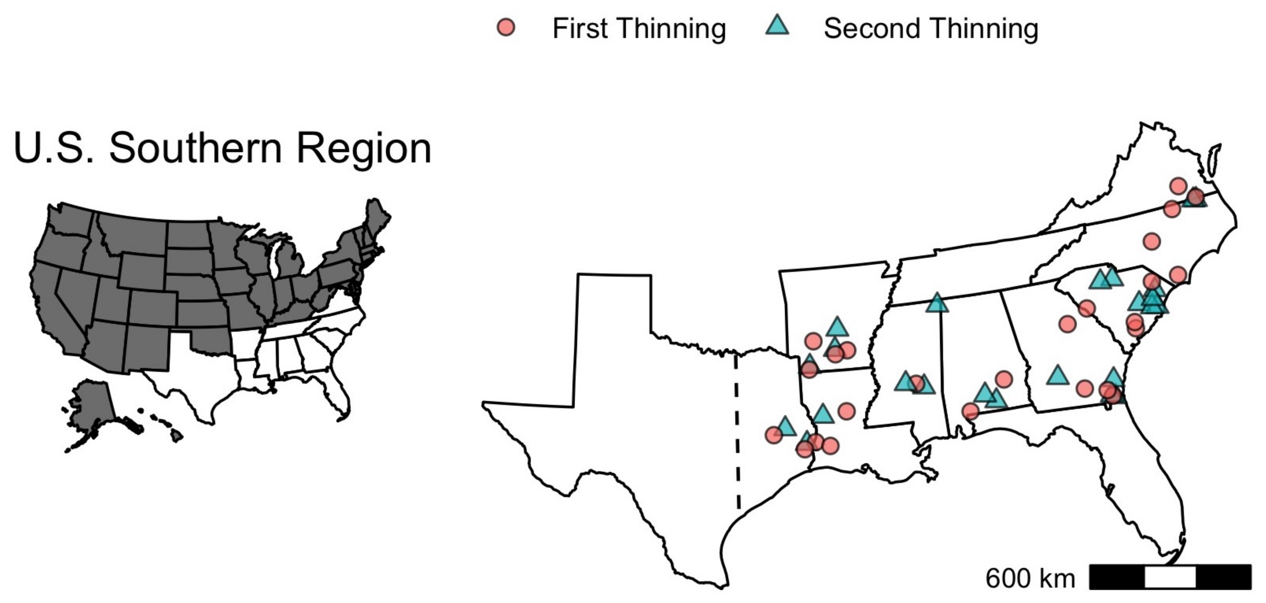
2.1. Study Design
2.2. Model Description
2.2.1. Dominant Height () Model
2.2.2. Stand Density
2.2.3. Basal Area
2.3. Estimation
- Obtain initial parameter estimations for the growth model independently of the other state variables, assuming the resulting yield follows a normal distribution with constant variance and mean explained by Equation (5). The initial value condition for each plot corresponds with the measured attributes at the thinning age.
- Project the plot yield and use these projections (instrumental variables) for the initial parameter estimations for finding the stand density growth Equation (7).
- Use the yield projections of and N from the two previous steps and estimate parameters for the basal area growth model (1).
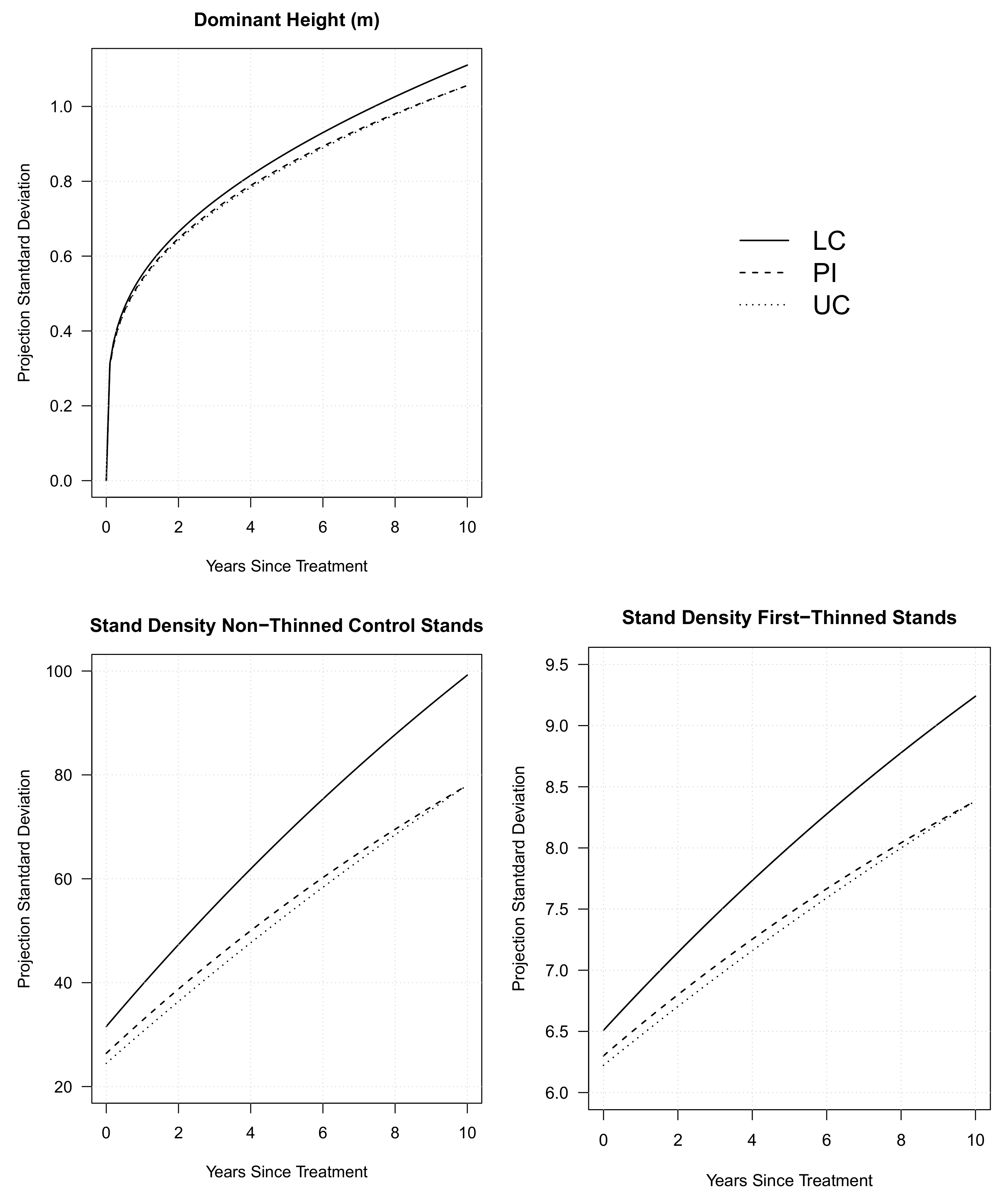
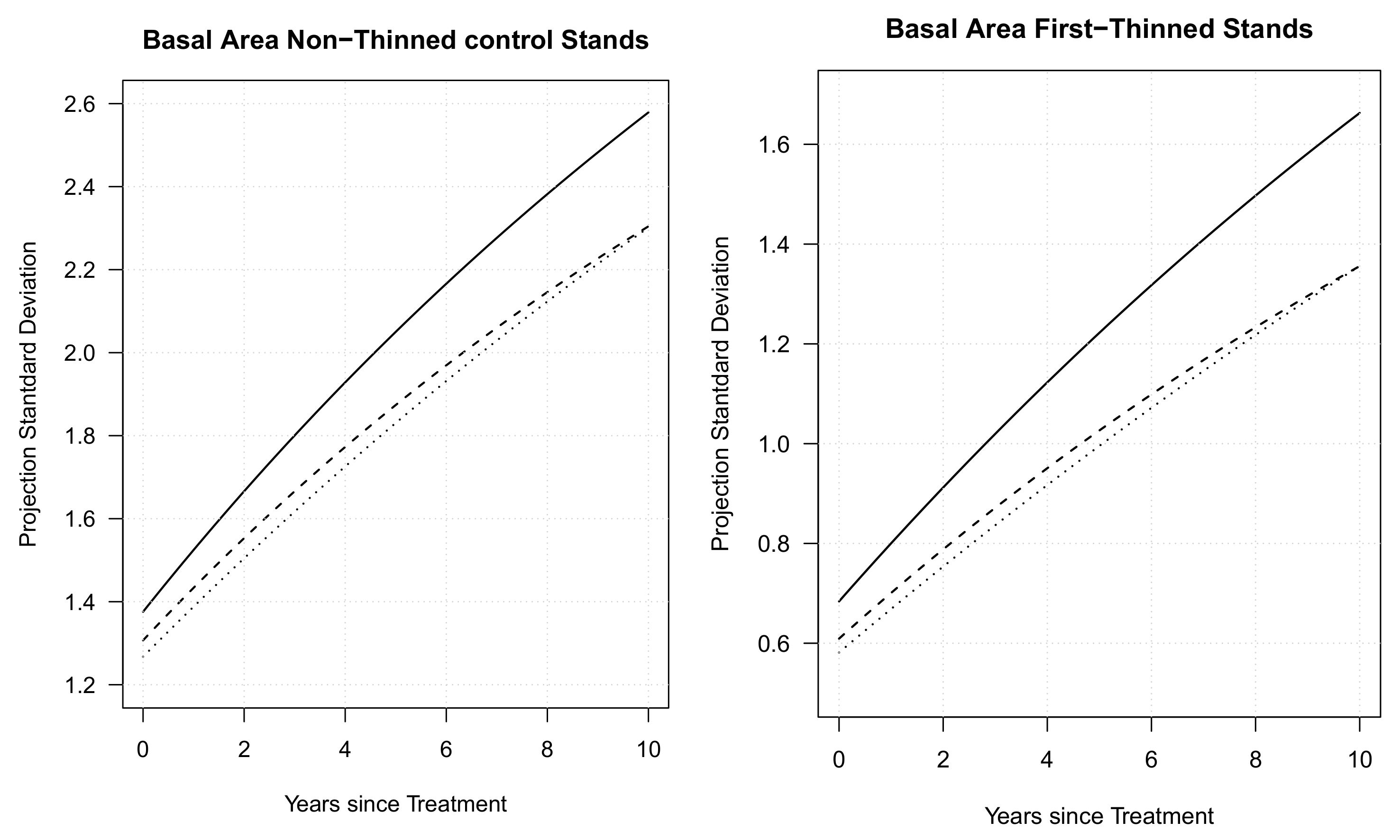
- Use the plot prediction residuals to explore and propose a function that predicts the standard deviations model error for each state.
- Use the previous plot level yield predictions to explore the type of cross-equation correlation for each combination of two responses.
- Use the multivariate normal distribution framework. The projected states are the mean, and the estimated standard deviations and cross-equation correlation are used to construct the respective covariance matrix for each plot observation.
- Use the maximum likelihood procedure to optimize the system parameters.
- The inverse of the Hessian matrix resulting from the optimization process should be used to obtain approximate standard errors for parameters. We found that the resulting Hessian matrix is invertible but, some of the diagonal elements produce negative values and a few returned huge numbers. In this case, the likelihood function may still contain considerable information about the models of interest, but through the Hessian the parameters are non-identifiable [28]. As not all the parameters were completely identifiable with the inverse of the Hessian matrix, we then compute the standard errors using a boostrap method. Five hundred random replications of the complete experiment data set were obtained sampling with replacement within physiographic region and thinning condition, then the model system was fitted with each replication and the fitted parameters were stored. The approximated standard error was obtained as:where, is the bootstrap standard error for the jth parameter, is the estimate jth paramater from the ith replicate data set, is the estimate parameter with the original data set, N is the number of replications.
2.4. Validation
3. Results
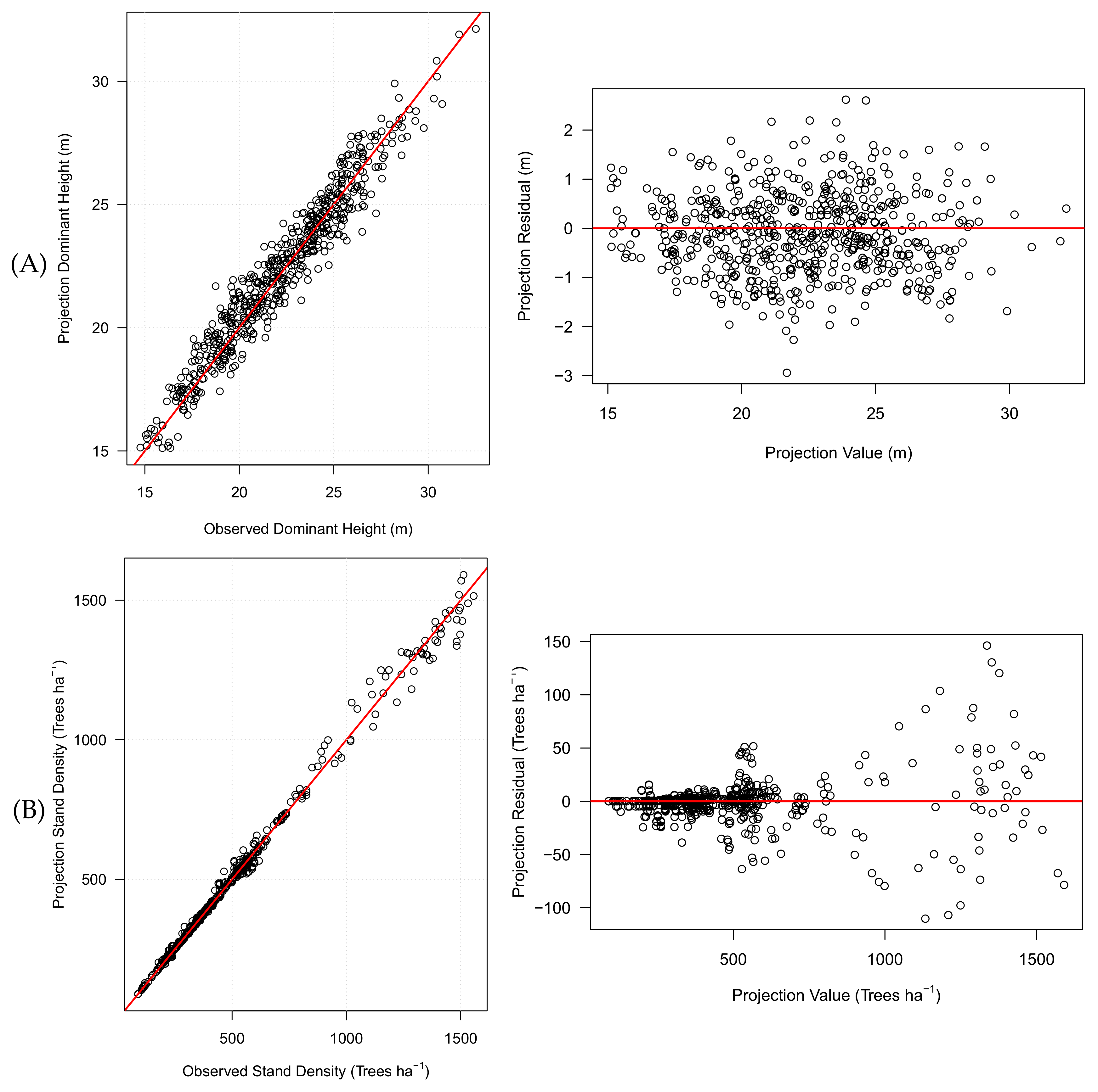
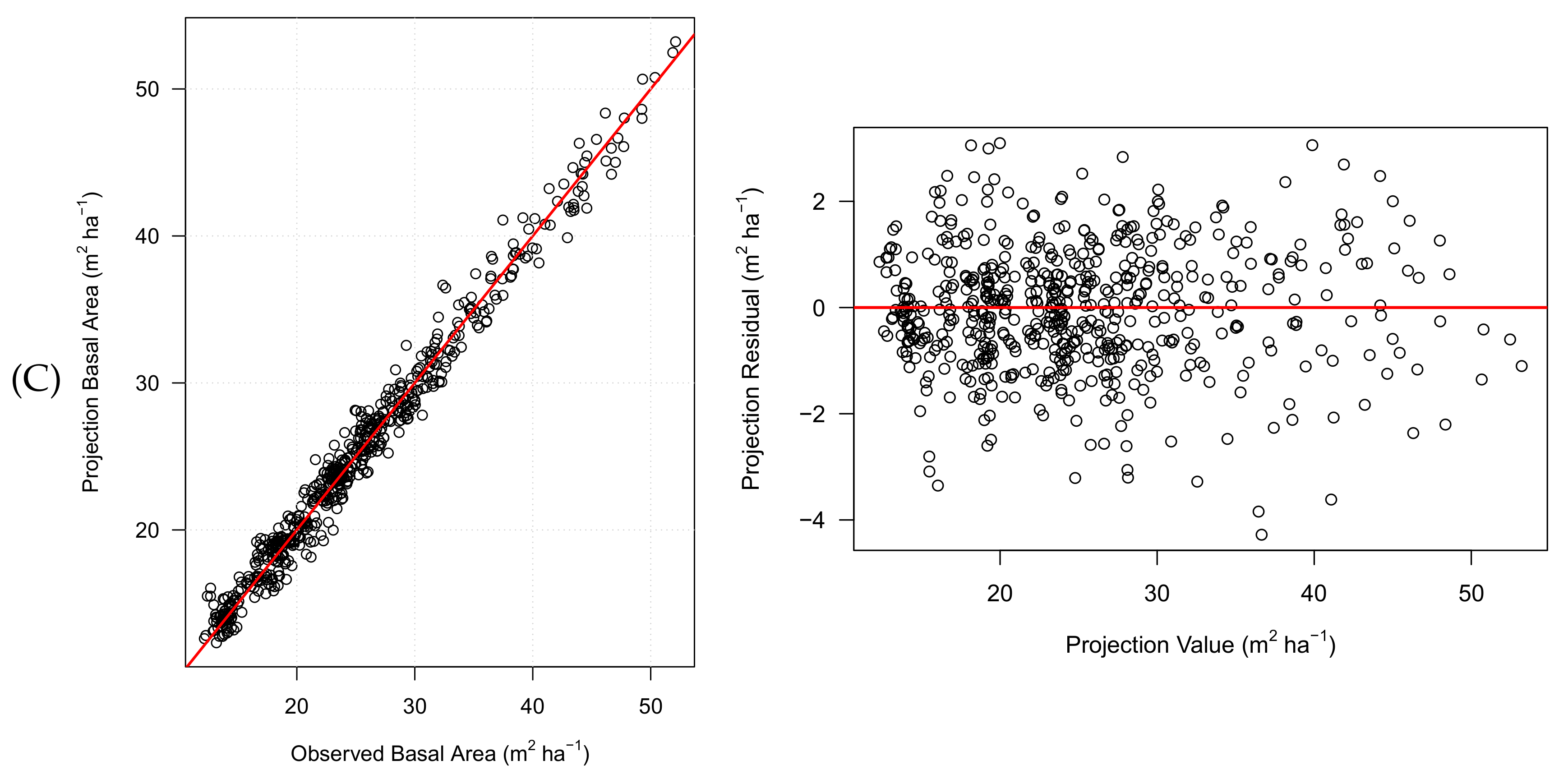
3.1. Validation
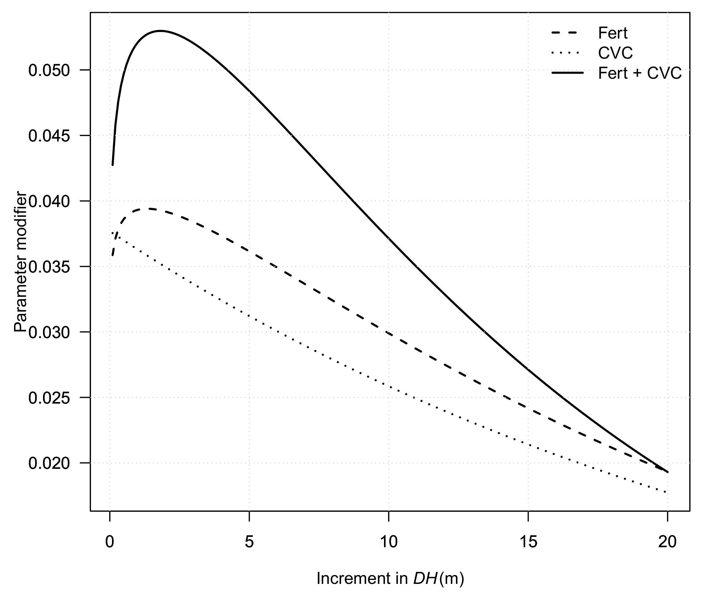
3.2. Treatment Effects
4. Discussion
5. Conclusions
Author Contributions
Funding
Data Availability Statement
Acknowledgments
Conflicts of Interest
Appendix A
Appendix A.1. Derivation of Equation (5)
Appendix A.2. Derivation of Equation (7)
Appendix A.3. Derivation of Equation (17)
Appendix A.4. Modifiers Equations
References
- Wear, D.N.; Greis, J.G. The southern forest futures project: Summary report. In The Southern Forest Futures Project: Summary Report; SRS-168; Forest Service Southern Research Station: Asheville, NC, USA, 2012; p. 68. [Google Scholar]
- Huggett, R.; Wear, D.N.; Li, R.; Coulston, J.; Liu, S. Forecasts of forest conditions. In The Southern Forest Futures Project: Technical Report; Wear, D.N., Greis, J.G., Eds.; General Technical Report SRS-GTR-178; USDA-Forest Service, Southern Research Station: Asheville, NC, USA, 2013; pp. 73–101. [Google Scholar]
- Stanturf, J.A.; Kellison, R.C.; Broerman, F.S.; Jones, S.B. Productivity of southern pine plantations. Where are we and how did we get here? J. For. 2003, 101, 26–31. [Google Scholar]
- Fox, T.R.; Eric, J.J.; Allen, L.H. The Evolution of Pine Plantation Silviculture in the Southern United States. In Southern Forest Science: Past, Present, and Future; Gen. Tech. Rep SRS-75; U.S. Department of Agriculture, Forest Service, Southern Research Station: Asheville, NC, USA, 2004; Volume 75, p. 394. [Google Scholar]
- Fox, T.R.; Lee Allen, H.; Albaugh, T.J.; Rubilar, R.; Carlson, C.A. Tree nutrition and forest fertilization of pine plantations in the Southern United States. South. J. Appl. For. 2007, 31, 5–11. [Google Scholar] [CrossRef]
- Cannell, M.; Dewar, R. Carbon allocation in trees: A review of concepts for modelling. Adv. Ecol. Res. 1994, 25, 59–104. [Google Scholar]
- Albaugh, T.J.; Fox, T.R.; Rubilar, R.A.; Cook, R.L.; Amateis, R.L.; Burkhart, H.E. Post-thinning density and fertilization affect Pinus taeda stand and individual tree growth. For. Ecol. Manag. 2017, 396, 207–216. [Google Scholar] [CrossRef]
- Sampson, D.; Allen, H. Regional influences of soil available water-holding capacity and climate, and leaf area index on simulated loblolly pine productivity. For. Ecol. Manag. 1999, 124, 1–12. [Google Scholar] [CrossRef]
- Jokela, E.J.; Martin, T.A.; Vogel, J.G. Twenty-five years of intensive forest management with Southern pines: Important lessons learned. J. For. 2010, 108, 338–347. [Google Scholar]
- Miller, J.H.; Zutter, B.R.; Zedaker, S.M.; Edwards, M.B.; Newbold, R.A. Growth and yield relative to competition for loblolly pine plantations to midrotation—A southeastern United States regional study. South. J. Appl. For. 2003, 27, 237–252. [Google Scholar] [CrossRef]
- Sharma, M.; Smith, M.; Burkhart, H.E.; Amateis, R.L. Modeling the impact of thinning on height development of dominant and codominant loblolly pine trees. Ann. For. Sci. 2006, 63, 349–354. [Google Scholar] [CrossRef]
- Pienaar, L. An Approximation of Basal Area Growth after Thinning Based on Growth in Unthinned Plantations. For. Sci. 1997, 25, 223–232. [Google Scholar]
- Amateis, R.L. Modeling Response to Thinning in Loblolly Pine Plantations. South. J. Appl. For. 2000, 24, 17–22. [Google Scholar] [CrossRef]
- Weiskittel, A.R. (Ed.) Forest Growth and Yield Modeling; Wiley: Hoboken, NJ, USA, 2011. [Google Scholar]
- Gyawali, N.; Burkhart, H.E. General Response Functions to Silvicultural Treatments in Loblolly Pine Plantations. Can. J. For. Res. 2015, 45, 252–265. [Google Scholar] [CrossRef]
- Ballard, T. A simple model for predicting stand volume growth response to fertilizer application. Can. J. For. Res. 1984, 14, 661–665. [Google Scholar] [CrossRef]
- Scolforo, H.F.; Montes, C.; Cook, R.L.; Lee Allen, H.; Timothy, J.; Rubilar, R.; Campoe, O. A New Approach for Modeling Volume Response from Mid-Rotation Fertilization of Pinus taeda L. Plantations. Forests 2020, 11, 646. [Google Scholar] [CrossRef]
- Amateis, R.L.; Liu, J.; Ducey, M.J.; Lee Allen, H. Modeling response to midrotation nitrogen and phosphorus fertilization in Loblolly Pine plantations. South. J. Appl. For. 2000, 24, 207–212. [Google Scholar] [CrossRef]
- Clutter, J.L.; Jones, E. Prediction of growth after thinning in old-field slash pine plantations. In Forest Service Research Paper; SE-217; Southern Forest Experiment Station: Asheville, NC, USA, 1980; p. 19. [Google Scholar]
- Garcia, O.; Burkhart, H.E.; Amateis, R.L. A biologically-consistent stand growth model for loblolly pine in the Piedmont physiographic region, USA. For. Ecol. Manag. 2011, 262, 2035–2041. [Google Scholar] [CrossRef]
- U.S. Environmental Protection Agency. Level III and IV Ecoregions by State. Available online: https://www.epa.gov/eco-research/level-iii-and-iv-ecoregions-state (accessed on 16 April 2021).
- Albaugh, T.J.; Fox, T.R.; Cook, R.L.; Raymond, J.E.; Rubilar, R.A.; Campoe, O.C. Forest fertilizer applications in the Southeastern Unites States from 1969 to 2016. For. Sci. 2019, 65, 335–362. [Google Scholar]
- Bertalanffy, V. Problems of organic growth. Nature 1949, 163, 156–158. [Google Scholar] [CrossRef]
- Pienaar, L.; Turnbull, K. The Chapmant-Richards generalization of von Bertalanffy’s growth model for basal area growth and yield in even-age stands. For. Sci. 1973, 19, 2–22. [Google Scholar]
- Garcia, O. A stochastic differential equation model for the height growth of forest stands. Biometrics 1983, 39, 1059. [Google Scholar] [CrossRef]
- Blanchard, P.; Devaney, R.; Hall, G. Differential Equations, 4th ed.; Brooks/Cole, Cengage Learning: Boston, MA, USA, 2012. [Google Scholar]
- R Core Team. R: A Language and Environment for Statistical Computing; R Foundation for Statistical Computing: Vienna, Austria, 2020. [Google Scholar]
- Kreutz, C.; Raue, A.; Kaschek, D.; Timmer, J. Profile likelihood in systems biology. FEBS J. 2013, 280, 2564–2571. [Google Scholar] [CrossRef]
- Gallagher, D. Uncertainty Estimaton in Forest Growth and Yield Systems. Ph.D. Thesis, University of Georgia, Athens GA, USA, 2019. [Google Scholar]
- Genz, A.; Bretz, F.; Miwa, T.; Mi, X.; Leisch, F.; Scheipl, F.; Hothorn, T. Mvtnorm: Multivariate Normal and t Distributions; R Package Version 1.1-0. Available online: https://cran.r-project.org/web/packages/mvtnorm/mvtnorm.pdf (accessed on 24 March 2021).
- Li, J. Assessing the accuracy of predictive models for numerical data: Not r nor r2, why not? Then what? PLoS ONE 2017, 12, e0183250. [Google Scholar] [CrossRef] [PubMed]
- Stage, A.; Crookston, N. Partitioning error components for accuracy-assessment of near-neighbor methods of imputation. For. Sci. 2007, 53, 62–72. [Google Scholar]
- Soderbergh, I.; Ledermann, T. Algorithms for simulating thinning and harvesting in five European individual-tree growth simulators: A review. Comput. Electron. Agric. 2003, 39, 115–140. [Google Scholar] [CrossRef]
- Franklin, O.; Aoki, K.; Seidl, R. A generic model of thinning and stand density effects on forest growth, mortality and net increment. Ann. For. Sci. 2009, 66, 815. [Google Scholar] [CrossRef]
- Bryars, C.; Maier, C.; Zhao, D.; Kane, M.; Borders, B.; Will, R.; Teskey, R. Fixed physiological parameters in the 3-PG model produced accurate estimates of loblolly pine growth on sites in different geographic regions. For. Ecol. Manag. 2013, 289, 501–514. [Google Scholar] [CrossRef]
- Subedi, S.; Fox, T.R. Modeling repeated fertilizer response and one-time midrotation fertilizer response in loblolly pine plantations using FR in the 3-PG process model. For. Ecol. Manag. 2016, 380, 90–99. [Google Scholar] [CrossRef]
- Albaugh, T.J.; Lee Allen, H.; Dougherty, P.M.; Johnsen, K.H. Long term growth responses of loblolly pine to optimal nutrient and water resource availability. For. Ecol. Manag. 2004, 192, 3–19. [Google Scholar] [CrossRef]
- Jokela, E.J.; Dougherty, P.M.; Martin, T.A. Production dynamics of intensively managed loblolly pine stands in the southern United States: A synthesis of seven long-term experiments. For. Ecol. Manag. 2004, 192, 117–130. [Google Scholar] [CrossRef]
- Albaugh, T.J.; Stape, J.L.; Fox, T.R.; Rubilar, R.A.; Allen, H.L. Midrotation Vegetation Control and Fertilization Response in Pinus taeda and Pinus elliottii across the Southeastern United States. South. J. Appl. For. 2012, 36, 44–53. [Google Scholar] [CrossRef]
- Allen, H.; Fox, T.; Campbell, R. What is ahead for intensive pine plantation silviculture in the South? South. J. Appl. For. 2005, 29, 62–69. [Google Scholar] [CrossRef]
- Jokela, E.J.; Martin, T.A. Effects of ontogeny and soil nutrient supply on production, allocation, and leaf area efficiency in loblolly and slash pine stands. Can. J. For. Res. 2000, 30, 1511–1524. [Google Scholar] [CrossRef]
| MRSP | Source | Stand Atribute | Equation | Type of Modifier | Base-Line Yield Model | Duration Effect | Estimation Procedure Base-Line and Modifier |
|---|---|---|---|---|---|---|---|
| Thin | [12] | BA | Equation (A29) | M | Counterpart stand | 0 < Z < inf | Independently |
| Thin | [13] | BA | Equation (A30) | A | Non-thinned stand | 0 < Z < inf | Independently |
| Thin | N | Equation (A31) | A | Non-thinned stand | 0 < Z < inf | Independently | |
| Thin | [15] | BA | Equation (A32) | M | Non-thinned stand | 0 < Z < k | Simultaneously |
| Thin | N | Equation (A33) | M | Non-thinned stand | 0 < Z < k | Simultaneously | |
| Fert | [16] | MV | Equation (A34) | M | Non-thinned stand | 0 < Z < inf | Independently |
| Fert | [15] | BA | Equation (A35) | M | Non-thinned stand | 0 < Z < inf | Simultaneously |
| Fert | [17] | V | Equation (A36) | M | Non-thinned stand | 0 < Z < inf | independently |
| Fert | [18] | DH | Equation (63) | A | Non-thinned stand | 0 < Z < k | independently |
| Fert | [18] | BA | Equation (64) | A | Non-thinned stand | 0 < Z < k | independently |
| Treatment Number | Thinning | Silvicultural Treatment |
|---|---|---|
| 1—Control | No | None |
| 2—Thin | Yes | None |
| 3—Fert | Yes | Fertilize (224.2 kg N ha−1 + 28 kg P ha−1) |
| 4—CVC | Yes | Prescribed for each location as conditions warrant and with follow-up to obtain excellent operational efficacy |
| 5—Fert + CVC | Yes | Fert + CVC |
| First-Thinning | Second-Thinning | ||||||||||
|---|---|---|---|---|---|---|---|---|---|---|---|
| Region | No. Plots | Age | DH | N | BA | No. Plots | Age | DH | N | BA | |
| LC | 60 | 11–17 | 14.6–21.2 | 1013–1735 | 10.8–44.7 | 55 | 16–25 | 17.6–25.6 | 430–717 | 11.4–33.7 | |
| PI | 20 | 14–15 | 12.9–21.1 | 1310–1626 | 11.1–44.6 | 10 | 21–27 | 19.6–23.1 | 534–578 | 15.6–33.2 | |
| UC | 45 | 12–17 | 13.8–19.6 | 919–1670 | 9.9–45.5 | 55 | 16–32 | 17.3–31.3 | 247–776 | 10.7–36.9 | |
| Parameter | Estimate | Boot SE | Lower Limit | Upper Limit | Parameter | Estimate | Boot SE | Lower Limit | Upper Limit |
|---|---|---|---|---|---|---|---|---|---|
| 1.7811 | 0.0902 | 1.6038 | 1.9584 | 20.7664 | 2.9640 | 14.9416 | 26.5912 | ||
| −2.742 × 10⁻⁵ | 2.954 × 10⁻⁷ | −2.799 × 10⁻⁵ | −2.683 × 10⁻⁵ | 25.4754 | 3.7524 | 18.1012 | 32.8496 | ||
| −0.8526 | 0.2716 | −1.3863 | −0.3189 | 14.1619 | 1.4066 | 11.3977 | 16.9261 | ||
| 0.2284 | 0.0754 | 0.0801 | 0.3766 | 0.1602 | 0.1014 | −0.0391 | 0.3594 | ||
| 0.0250 | 0.0066 | 0.0119 | 0.0380 | −0.3137 | 0.0577 | −0.4271 | −0.2002 | ||
| 0.0150 | 0.0047 | 0.0058 | 0.0243 | −0.0352 | 0.0081 | −0.0510 | −0.0194 | ||
| 0.1618 | 0.1033 | −0.0412 | 0.3648 | −0.0275 | 0.0099 | −0.0469 | −0.0081 | ||
| −0.0936 | 0.0130 | −0.1192 | −0.0680 | −4.2440 | 0.1455 | −4.5298 | −3.9581 | ||
| 0.0439 | 0.0043 | 0.0355 | 0.0524 | −0.6748 | 0.0596 | −0.7920 | −0.5576 | ||
| 11.5935 | 1.8150 | 8.0267 | 15.1604 | 0.5051 | 0.0504 | 0.4061 | 0.6041 | ||
| 4.0936 | 1.3153 | 1.5088 | 6.6783 | 4.8698 | 0.4565 | 3.9728 | 5.7668 | ||
| 3.6310 | 0.5343 | 2.5809 | 4.6811 | 0.3226 | 0.0284 | 0.2667 | 0.3784 | ||
| −0.0198 | 0.0031 | −0.0258 | −0.0138 | 8.0178 | 0.8514 | 6.3447 | 9.6910 | ||
| 0.1493 | 0.0690 | 0.0138 | 0.2849 | 0.2732 | 0.0290 | 0.2162 | 0.3302 | ||
| 0.0370 | 0.0123 | 0.0128 | 0.0612 | 0.0950 | 0.0101 | 0.0752 | 0.1148 | ||
| 0.0398 | 0.0193 | 0.0020 | 0.0777 | 0.0233 | 0.0019 | 0.0196 | 0.0270 | ||
| 11.4625 | 3.9969 | 3.6080 | 19.3171 | −0.1528 | 0.0148 | −0.1820 | −1.1236 | ||
| 0.0556 | 0.0119 | 0.0322 | 0.0790 | 0.2674 | 0.0224 | 0.2234 | 0.3114 | ||
| 2.379 × 10⁻⁸ | 1.096 × 10⁻¹⁴ | 2.379 × 10⁻⁸ | 2.379 × 10⁻⁸ | 0.2172 | 0.0211 | 0.1756 | 0.2587 | ||
| 0.1047 | 0.0252 | 0.0551 | 0.1542 |
| Response | Group/Treatment | n | Variance Explained (%) | Residual Mean | RMSD |
|---|---|---|---|---|---|
| DH (m) | LC | 335 | 96.3 | −0.0646 | 0.649 |
| PI | 105 | 98.0 | 0.117 | 0.519 | |
| UC | 393 | 95.5 | −0.0645 | 0.787 | |
| Non-Thin | 160 | 96.6 | −0.0289 | 0.673 | |
| Thin | 162 | 96.1 | −0.162 | 0.679 | |
| Fert | 169 | 95.9 | −0.0421 | 0.751 | |
| CVC | 169 | 96.1 | −0.0578 | 0.729 | |
| Fert+CVC | 173 | 96.4 | 0.0759 | 0.682 | |
| All | 833 | 96.2 | −0.0416 | 0.704 | |
| N (trees ha−1) | LC | 335 | 99.5 | −2.07 | 23.4 |
| PI | 105 | 99.7 | 4.73 | 19.9 | |
| UC | 393 | 99.8 | −1.05 | 14.0 | |
| Non-Thin | 160 | 99.1 | −1.25 | 37.9 | |
| Thin | 162 | 99.8 | −0.566 | 7.67 | |
| Fert | 169 | 99.4 | −0.866 | 12.1 | |
| CVC | 169 | 99.6 | 0.340 | 9.61 | |
| Fert+CVC | 173 | 99.5 | −1.32 | 11.4 | |
| All | 833 | 99.7 | −0.730 | 19.1 | |
| BA (m2 ha−1) | LC | 335 | 98.4 | −0.0196 | 1.01 |
| PI | 105 | 98.9 | 0.0483 | 0.907 | |
| UC | 393 | 98.6 | −0.155 | 1.06 | |
| Non-Thin | 160 | 96.1 | −0.140 | 1.32 | |
| Thin | 162 | 96.9 | −0.0386 | 0.911 | |
| Fert | 169 | 97.0 | −0.101 | 0.955 | |
| CVC | 169 | 97.2 | −0.0404 | 0.924 | |
| Fert + CVC | 173 | 97.1 | −0.0582 | 0.975 | |
| All | 833 | 98.6 | −0.0751 | 1.03 |
Publisher’s Note: MDPI stays neutral with regard to jurisdictional claims in published maps and institutional affiliations. |
© 2021 by the authors. Licensee MDPI, Basel, Switzerland. This article is an open access article distributed under the terms and conditions of the Creative Commons Attribution (CC BY) license (https://creativecommons.org/licenses/by/4.0/).
Share and Cite
Zapata-Cuartas, M.; Bullock, B.P.; Montes, C.R.; Kane, M.B. A Dynamic Stand Growth Model System for Loblolly Pine Responding to Mid-Rotation Treatments. Forests 2021, 12, 556. https://doi.org/10.3390/f12050556
Zapata-Cuartas M, Bullock BP, Montes CR, Kane MB. A Dynamic Stand Growth Model System for Loblolly Pine Responding to Mid-Rotation Treatments. Forests. 2021; 12(5):556. https://doi.org/10.3390/f12050556
Chicago/Turabian StyleZapata-Cuartas, Mauricio, Bronson P. Bullock, Cristian R. Montes, and Michael B. Kane. 2021. "A Dynamic Stand Growth Model System for Loblolly Pine Responding to Mid-Rotation Treatments" Forests 12, no. 5: 556. https://doi.org/10.3390/f12050556
APA StyleZapata-Cuartas, M., Bullock, B. P., Montes, C. R., & Kane, M. B. (2021). A Dynamic Stand Growth Model System for Loblolly Pine Responding to Mid-Rotation Treatments. Forests, 12(5), 556. https://doi.org/10.3390/f12050556


