Spatial and Temporal Changes in Vegetation in the Ruoergai Region, China

Abstract

Timely monitoring of the changes in coverage and growth conditions of vegetation (forest, grass) is very important for preserving the regional and global ecological environment. Vegetation information is mainly reflected by its spectral characteristics, namely, differences and changes in green plant leaves and vegetation canopies in remote sensing domains. The normalized difference vegetation index (NDVI) is commonly used to describe the dynamic changes in vegetation, but the NDVI sequence is not long enough to support the exploration of dynamic changes due to many reasons, such as changes in remote sensing sensors. Thus, the NDVI from different sensors should be scientifically combined using logical methods. In this study, the Global Inventory Modeling and Mapping Studies (GIMMS) NDVI from the Advanced Very High Resolution Radiometer (AVHRR) and Moderate-resolution Imaging Spectroradiometer (MODIS) NDVI are combined using the Savitzky–Golay (SG) method and then utilized to investigate the temporal and spatial changes in the vegetation of the Ruoergai wetland area (RWA). The dynamic spatial and temporal changes and trends of the NDVI sequence in the RWA are analyzed to evaluate and monitor the growth conditions of vegetation in this region. In regard to annual changes, the average annual NDVI shows an overall increasing trend in this region during the past three decades, with a linear trend coefficient of 0.013/10a, indicating that the vegetation coverage has been continuously improving. In regard to seasonal changes, the linear trend coefficients of NDVI are 0.020, 0.021, 0.004, and 0.004/10a for spring, summer, autumn, and winter, respectively. The linear regression coefficient between the gross domestic product (GDP) and NDVI is also calculated, and the coefficients are 0.0024, 0.0015, and 0.0020, with coefficients of determination (R²) of 0.453, 0.463, and 0.444 for Aba, Ruoergai, and Hongyuan, respectively. Thus, the positive correlation coefficients between the GDP and the growth of NDVI may indicate that increased societal development promotes vegetation in some respects by resulting in the planting of more trees or the promotion of tree protection activities. Through the analysis of the temporal and spatial NDVI, it can be assessed that the vegetation coverage is relatively large and the growth condition of vegetation in this region is good overall.

1. Introduction

Global climate change, such as increasing atmospheric temperature, irregular precipitation, and changes in sunshine durations, has been detected, and nowadays the climate change is happening more obviously than the past several decades [1,2,3,4,5,6]. The changing climate has significantly influenced the growth of vegetation, and the mechanisms of climate change influencing vegetation are complex because vegetation can be influenced by the changing climate and can also adapt to various environments [7,8,9]. It has been proven that the increasing trend of global warming has influenced vegetation, such as changes in the phenology of vegetation (greening, flowering, and leaf fall) [10,11,12,13,14]. Since the increasing trend will last for the next several decades, it is of vital importance to monitor the changes in vegetation, as vegetation coverage is closely correlated with the gross primary productivity, biosphere, and ecological cycle, which are the dominant factors for balancing ecosystems [15,16,17,18,19]. Thus, timely monitoring of the growth coverage and growth condition of vegetation and acknowledging the temporal and spatial changes in vegetation will not only benefit the development of society but also promote the quality of the ecological environment.

Satellite remote sensing has long been adopted for observing vegetation because it can collect large-area data over long time periods [20,21,22,23]. SRS can detect ground objects using the combination of spectral bands of images ranging from the visible to near-infrared and infrared [24]. The vegetation index is commonly designed to maximize the characteristics of vegetations while minimizing other effects, such as soil disturbance and atmospheric effects [25,26]. The vegetation index is a simple and efficient indicator for assessing and evaluating vegetation coverage, biomass, and soil background on the ground [27,28,29,30,31]. The normalized difference vegetation index (NDVI) is calculated as a ratio between the red and near infrared values in traditional fashion: (NIR − R)/(NIR + R). The NDVI is used to estimate the density of green on an area of land, and it is closely related to green vegetation biomass, vegetation growth status, and vegetation photosynthetic capacity [32,33,34,35]. NDVI reflects the background influence of the plant canopy, and it is widely used for the retrieval of information regarding vegetation physical parameters and surface vegetation coverages [35,36]. Long time series of NDVI datasets have been used to explore global and regional environmental changes, such as dynamic changes in vegetation and land cover changes. However, the time series of the NDVI dataset contains considerable noise ascribed to atmospheric conditions, such as cloud and aerosol scatter. Additionally, the current Global Inventory Modeling and Mapping Studies (GIMMS) NDVI from Advanced Very High Resolution Radiometer (AVHRR) sensors (National Aeronautics and Space Administration, Washington DC, USA) is a NDVI product available for the period spanning from 1981 to 2006, and the Moderate-resolution Imaging Spectroradiometer (MODIS) NDVI ranges from 2000 to present. Thus, the usage of a single NDVI dataset is not enough if there is a need to explore the temporal changes of a relatively long period [37,38,39]. Therefore, it is necessary to determine an appropriate method of fusing and generating the standard sequence of NDVI datasets based on different sensors. Further analysis should be conducted based on the rebuilt NDVI sequence.

Several studies have obtained long time series of NDVI datasets over 30 continuous years. However, most of the current studies are based on the comprehensive application of a single dataset, and thus, there is a need to investigate long-term fusions of two or more NDVI datasets when the adoption of a single NDVI dataset can hardly meet the temporal scales (e.g., the NDVI of 1981 to present is needed). There have been comprehensive applications using different sources of NDVI data, and the analysis and comparison of different time scales have proven that there are close correlation relationships between these NDVI products [40,41,42]. Therefore, the synthesis of continuous NDVI products is possible by fusing NDVI datasets from multiple sources into a uniform set. The Landsat The Enhanced Thematic Mapper Plus NDVI and NDVI calculated by Moderate-resolution Imaging Spectroradiometer (MODIS) products were normalized and compared, and the results show that the NDVI from MODIS and its combination with different sources can be adopted for time-series analysis [43]. Kevin et al. analyzed the difference between the NDVI from MODIS and the AVHRR sensors on the National Oceanic and Atmospheric Administration (NOAA) satellites and established a good relationship model using the two data sources. The different vegetation types using the two sensors from MODIS and NOAA in the United States for the same time period were compared, and the results showed that the synthetic 16-day data were similar and showed good linear relationships [44]. Michele et al. compared the two instruments from the point of view of the user interested in operational crop monitoring using PROBA-V (QinetiQ Space Belgium, Paris, France) instead of SPOT (Spot Image, Toulouse, France), and the results showed a high agreement between these two instruments [45]. Caleb et al. conducted a methodology based on a dynamic framework that was proposed to incorporate additional sources of information into the NDVI time series of agricultural observations for the estimation of phenology [46]. Mao et al. constructed the yearly maximum GIMMS NDVI sequence of the AVHRR and MODIS in Northeast China from 1982 to 2009 using a per-pixel unary linear regression model [47]. Thus, it is possible to obtain a continuous NDVI product with high consistency by fusing the data from a similar remote sensing system. A reconstructed long time series of NDVI datasets can be used to monitor the dynamic changes in vegetation and land transfer types by revealing important information and knowledge. To date, only a few studies have focused on the reconstruction of NDVI time series using two or more NDVI datasets that cover the whole Ruoergai wetland area (RWA). The NDVIs from AVHRR, MODIS, and SPOT are available for the RWA, and they are important for specific vegetation types, vegetation growth characteristics, topography, climate, and other factors. They are all suitable for monitoring the dynamic changes in vegetation in the RWA. The multiple sources of NDVI can reflect the characteristics of vegetation changes, and their respective characteristics can be investigated and obtained to perform efficient data fusion.

To the best of our knowledge, the influencing factors that characterize long-term vegetation changes have not been well explored or investigated in the RWA. The ecological environment of the RWA is vulnerable to the changing climate, as it belongs to high-altitude areas. Meanwhile, the single dataset of NDVI can hardly support the analysis of vegetation in the RWA from 1982 to present. Thus, further in-depth and extensive research is urgently needed to analyze the change and trend of the NDVI in the RWA. Two different NDVI datasets: GIMMS NDVI (1982 to 2006) and MODIS NDVI (2000 to 2018) have been adopted for analyzing the spatial and temporal changes of vegetation in the RWA. In this study, the objectives were to try (1) to apply linear regression analysis of two NDVI datasets between GIMMS and MODIS NDVI of the RWA; (2) to reconstruct the NDVI sequence through the Savitzky–Golay (SG) filtering method using the GIMMS NDVI and MODIS NDVI in RWA; and (3) to analyze the spatial, temporal, and seasonal changes with the trends of vegetations in RWA at different counties.

2. Material and Methods

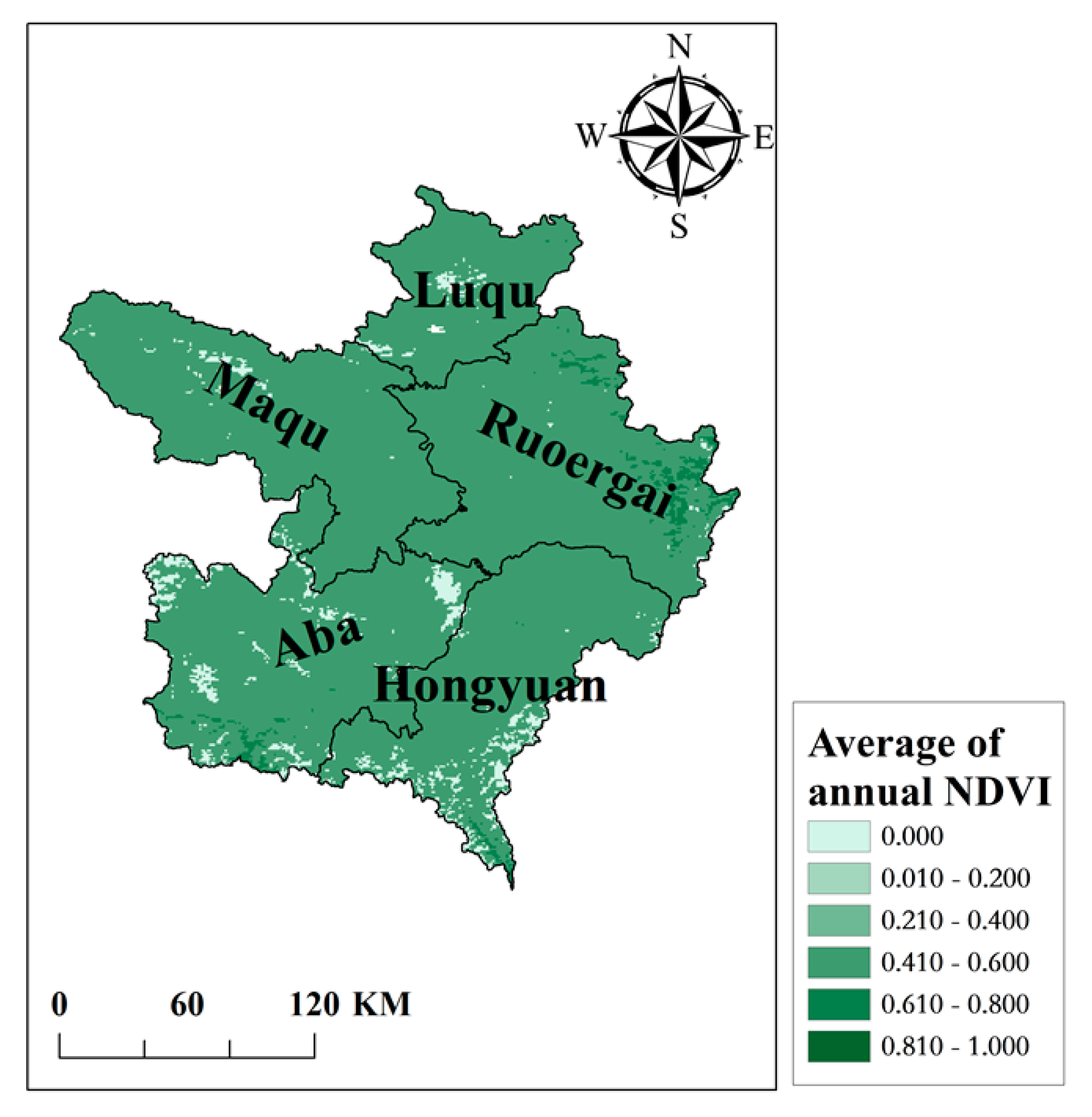
2.1. Study Area

The RWA is in the northern part of Sichuan Province, which is on the edge of the Qinghai–Tibet Plateau (Figure 1). The south (north) is high (low) in altitude, ranging from 2500 to 5000 m [48]. The climate in this area is a humid monsoon, as it is in the plateau cold zone, with cold winters and cool summers, along with abundant solar radiation, rain, and hot temperatures. The annual rainfall is between 500 and 600 mm/year, with an annual average temperature of 1.4 °C. The average annual sunshine hours is 2389, and the annual average evaporation is 1232 mm [49]. The maximum wind force is 11 m/second, and the wind direction is mostly a northwest wind. Freezing starts in late September each year, with a maximum frozen soil depth of 72 cm, and can only be completely thawed in mid-May [50]. The vegetation in this region is dominated by alpine meadows and marsh vegetation, with a total wetland area of approximately 53 million square kilometers. There are five counties in this area, namely, Aba County, Hongyuan County, Ruoergai County, Luqu County, and Maqu County.

Since 1970, the ecological and environmental problems in the RWA have become increasingly serious. Thus, the RWA was established as a nature reserve in 1994, and a series of ecological restoration measures have been implemented in order to improve the growth of vegetation and increase vegetation coverage [51]. In general, the vegetation growth conditions and evolution trends in the RWA are of great significance to local tourism, animal husbandry, transportation, urban development, and even the sustainable economic and ecological development of the entire southwestern region. Therefore, the vegetation change in the RWA deserves substantial attention.

2.2. Data Source

2.2.1. NDVI Data Source

The remote sensing-obtained NDVI data used in this study are from the GIMMS and MODIS (Santa Barbara Remote Sensing, NASA, USA) NDVI. The GIMMS NDVI can be assessed from the Heihe Project Data Management Center and the Cold and Arid Regions Science Data Center (http://westdc.westgis.ac.cn). The data have been corrected through radiometric correction and cloud removal for quality control. The international maximum value synthesis method is adopted to obtain the NDVI data every half month, and the data spatial resolution is 8 km. The MODIS remote sensing data were downloaded from the vegetation index data (MOD13A3) provided by the National Space Administration (NASA), of which the time resolution was 16 days and the spatial resolution was 1 km (https://ladsweb.modaps.eosdis.nasa.gov/missions-and-measurements/products/MOD13A3/). The data have undergone preprocessing such as the elimination of ground reflections and noise.

2.2.2. Vegetation Types

The vector data of this region were obtained from the National Geographic Information Resource Directory Service System (http://www.webmap.cn/commres.do?method=result100W). The vegetation type data source was from the project “1:1,000,000 China Vegetation Atlas” compiled by the Resource and Environmental Science Data Center of the Chinese Academy of Sciences (CAS) (http://www.resdc.cn). The vegetation types of this region contain nine main types of cultivated vegetation, namely, broad-leaved forest, swamp, grassland, shrub, meadow, alpine vegetation, and coniferous forest. To match the NDVI data, the resolution of the vegetation type data was resampled in ARCGIS (version 10.4, Esri, USA) (https://www.arcgis.com/index.html), and then mask extraction was performed to obtain the vegetation type of this region.

2.3. Method

2.3.1. The Mean Method and Resampling Method

The average annual vegetation NDVI and seasonal average vegetation NDVI in the RWA from 2000 to 2015 were calculated by means of the monthly NDVI value. The formula is defined as follows:

$$\overline{NDV{I}_x}=\frac{{{\displaystyle \sum }}_{i=1}^{12}NDV{I}_i}{12}$$

(1)

In the equation, the variable i varies from 1 to 12, $\overline{NDV{I}_x}$ is the average annual NDVI, $NDV{I}_i$ is the NDVI of the i-th month, and i is the month number. The seasonal averages are defined as spring (from March to May), summer (from June to August), autumn (from September to November), and winter (from December to February).

Since the spatial resolution of GIMMS and MODIS NDVI was different, the resampling operation should be performed to achieve consistency. Therefore, the GIMMS NDVI was sampled as 1 km in ArcGIS. Since the MODIS NDVI and the GIMMS NDVI have the same temporal periods from 2000 to 2006, the multiyear average value of seven years was calculated for each pixel to achieve continuity between the two datasets from January to December. The linear fitting formula for each month is defined as follows:

$$NDV{I}_G=a\times \left(NDV{I}_M\right)+b$$

(2)

where $NDV{I}_G$ is the value of GIMMS NDVI and $NDV{I}_M$ is the MODIS NDVI. In addition, a is the coefficient, and b is the constant.

2.3.2. Savitzky–Golay Method

It is necessary to determine certain filtering parameters, then use polynomials, and finally realize the filtering method of least square fitting. This method was proposed by Savitzky and Golay in 1964 and improved by Chen Equal in 2004 to make it more suitable for fitting vegetation growth curves [52]. The formula is defined as follows:

$$Y_j^{*}=\frac{{{\displaystyle \sum }}_{i=-m}^{i=m}{C}_i{Y}_j+i}{N}$$

(3)

where $Y_j$ is the initial NDVI; $Y_j^{*}$ is the fitted NDVI value; m represents the size of the sliding window; C is the filter coefficient of the i-th NDVI value; N represents the length of the filter, meaning the width of the sliding array is (2 × m + 1); and j represents the coefficient of the initial NDVI array.

2.3.3. Workflow of Data Processing

The whole workflow of data processing can be divided into four parts (Figure 2). First, the NDVIs from GIMMS and MODIS were preprocessed to achieve the same format, projection, and coordinate system, which are necessary for information extraction. To achieve this, the MODIS Reprojection Tool (MRT) tool was adopted for preprocessing, such as data cropping and projection coordinate conversion of the MODIS NDVI data to ensure a coordinate system consistent with that of the GIMMS NDVI. The vegetation type data and administrative division vector data were used as masks to extract vectors from the RWA. Second, the GIMMS NDVI was resampled to the same resolution as MODIS, and SG was adopted to reconstruct the NDVI time-series data, which aims to improve the quality of the data by removing noise, clouds, and aerosols. Third, the unary linear regression method was used for reconstructing the long-term NDVI sequence in the RWA. For vegetation type data and administrative division data, the collected vegetation type data were combined with the administrative division data to extract the vegetation type data in the RWA. Thus, the map of vegetation types in the RWA was constructed. At the time intersection of the two NDVI datasets from 2000 to 2006, mean value synthesis was performed to obtain the year-by-year NDVI of the RWA from 1982 to 2018, and unary linear regression was used to unify the two datasets. Finally, according to the unified dataset, from the seasonal changes of spring, summer, autumn, and winter and the different time scales of the annual change, the characteristics of the time change and spatial differentiation of the study area were analyzed. The results of the RWA were analyzed through the following four aspects:

(1)

The NDVI data were first preprocessed, and for the results of the filtering process, the GIMMS NDVI was processed using the SG filtering method. The results of the same time period were compared with the NDVI of MODIS to ensure that the accuracy of the filtered data was improved.

(2)

The vegetation type, shape file, and NDVI data were all processed and extracted for the RWA in five counties: Aba County, Hongyuan County, Ruoergai County, Luqu County, and Maqu County.

(3)

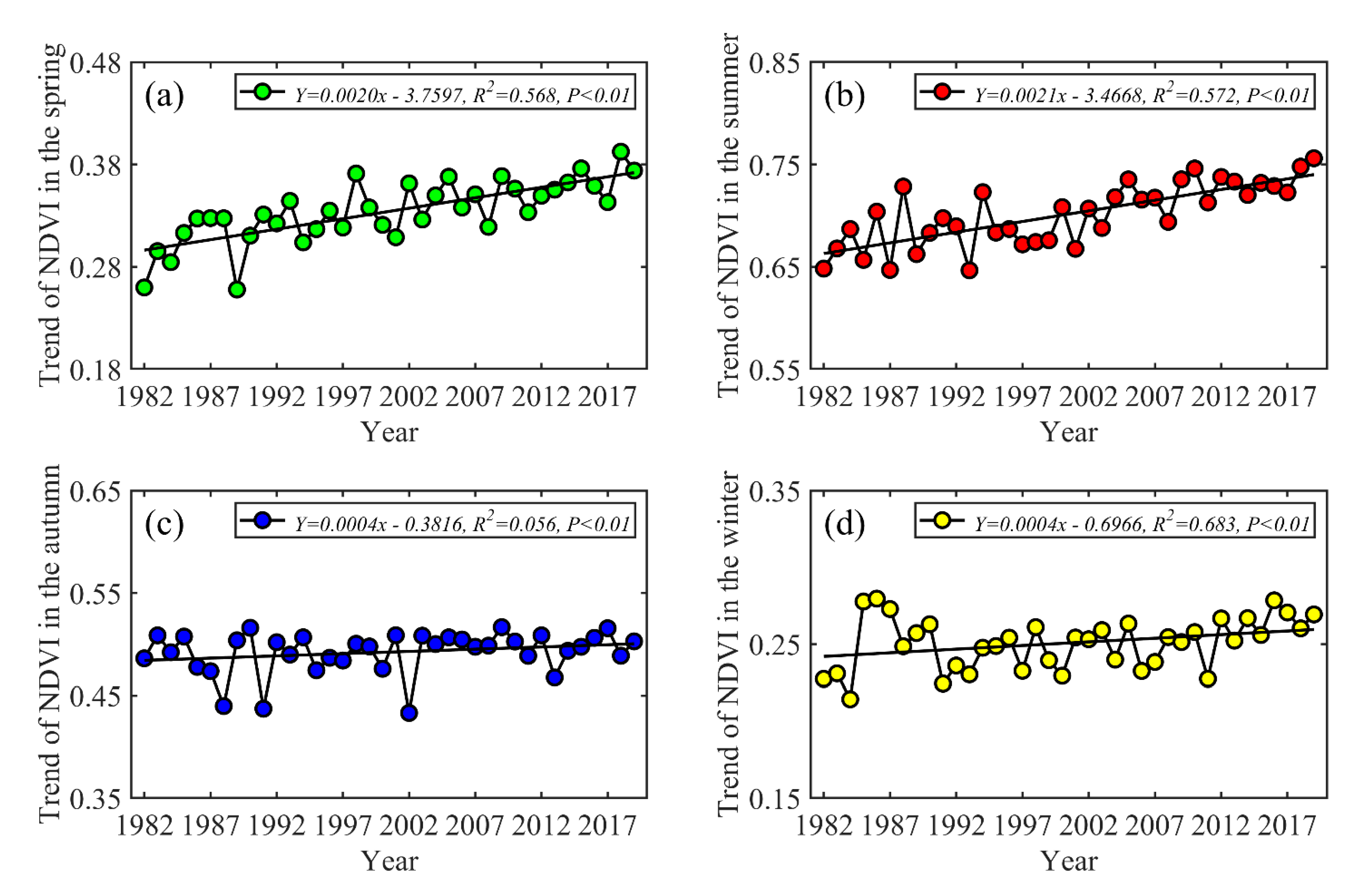
The temporal change in vegetation coverage using different scales, including the four seasons and interannual changes in the NDVI of the RWA was analyzed. Spring was defined as being from March to May, summer was defined as being from June to August, autumn was defined as being from September to November, and winter was defined as being from December to February.

(4)

The spatial change in vegetation coverage, including the spatial distribution and change trend of its NDVI value in different seasons and at different scales, was evaluated; additionally, the four seasons and the whole year for the different districts and counties in the RWA were analyzed.

(5)

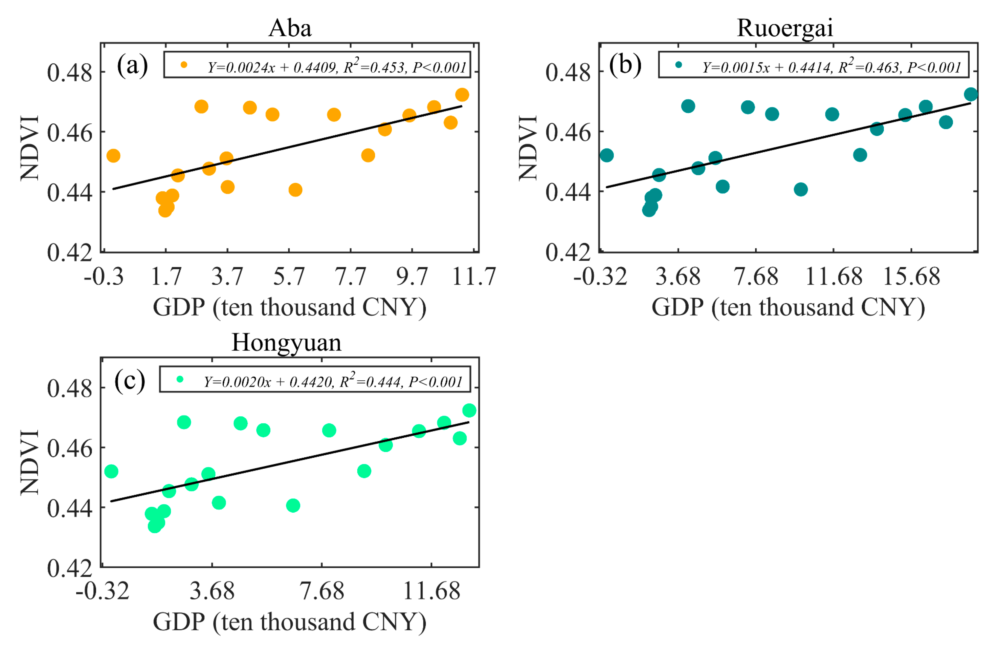
The contributions of social influencing factors were analyzed. The gross domestic product (GDP) was obtained from the National Bureau of Statistics (https://data.stats.gov.cn/), and the detailed data was recorded in country, year, GDP (ten thousand CNY) forms in an independent file. These data were not all available for all counties, and thus, only counties with GDP data were further selected for linear regression. The linear relationships were built between GDP and the NDVI values and the coefficients were obtained.

3. Results

3.1. Preprocessing of the NDVI

The long time series of the GIMMS and MODIS NDVI of the RWA are shown and compared (Figure 3a,b). The data were resampled into monthly values to better match the consistency of the two different sensors that provided the NDVI sequence. The GIMMS NDVI before and after the filtering process is also shown and compared with the MODIS NDVI from February 2002 to September 2006 (Figure 3c,d).

It can be acknowledged that the curve of GIMMS before SG filtering had poor continuity and prominent abnormal values compared with MODIS. To be more specific, the GIMMS NDVI values before the filtering process were all lower at the peak and bottom than those of MODIS NDVI, and these NDVI values meant that the GIMMS NDVI was not well corrected compared with MODIS NDVI. When the GIMMS NDVI was filtered using the SG method, the data values of GIMMS were similar to those of MODIS. Thus, the current NDVI sequence of GIMIMS for the entire time period (January 1982 to December 2006) should be filtered to remove the effects ascribed from different sensors using the SG filtering method. Thus, the long time series of the NDVI sequence was obtained via the above filtering method (1982–2020).

3.2. Temporal Changes of the NDVI in the RWA

The monthly average NDVI values and the seasonal average NDVI values of the RWA were calculated using the reconstructed NDVI sequence from 1982–2020. The vegetation of this region was analyzed using the NDVI sequence for spring, summer, autumn, and winter (Figure 4). The coefficients of determination and significance values were calculated using the inbuilt function regress in MATLAB (version 2019b, University of New Mexico, Albuquerque, USA). It can be directly observed that the NDVI values significantly differed between the four seasons in the RWA, of which the rate of the NDVI in summer increased the fastest and the rate of the NDVI in autumn increased the slowest, as the calculated coefficients of determination of these two seasons were the highest and lowest among the four seasons.

The linear regression models were built between time and the NDVI sequence and the ratios were 0.020, 0.021, 0.004, and 0.004/10a and the R² were 0.568, 0.572, 0.056, and 0.683 for spring, summer, autumn, and winter, respectively. The vegetation trends in spring and summer were maybe greater than those in autumn and winter. Based on the interannual variation characteristics of the seasonal average NDVI, the seasonal variation trends of the NDVI in the RWA were different from 1982 to 2019. The seasonal changes in the NDVI value in spring decreased dramatically in 1989. The minimum, maximum, and mean values of the NDVI were 0.258, 0.392, and 0.343 for spring, respectively. The growth trends of the NDVI varied significantly between approximately 1988 and 1994, which may be correlated with the changes in climate conditions. After 2000, although there was still an alternating trend of rising and falling, the overall summer NDVI trend was relatively good. The minimum, maximum, and mean values of the NDVI were 0.647, 0.756, and 0.721 in summer, respectively. In autumn, there were three decreasing points (1988, 1991, and 2002), and the corresponding NDVI values were 0.440, 0.437, and 0.433, respectively. The overall change trend of the NDVI in autumn was not obvious. The minimum, maximum, and mean values of the NDVI were 0.433, 0.517, and 0.506 in autumn, respectively. The increasing trend of the NDVI in winter was slightly higher than that in autumn, and the minimum, maximum, and mean values of the NDVI were 0.214, 0.258, and 0.279, respectively.

The annual average NDVI values from 1982 to 2018 were calculated to explore the overall change trend of vegetation in the RWA (Figure 5). The curve of the NDVI sequence was volatile from 1982 to 1998, of which the NDVI increased and decreased one year later. The average NDVI decreased first from 1998, reached its lowest value in 1999, and then increased until 2005. The NDVI values varied between 0.405 and 0.472, and the overall trend of the NDVI sequence in the RWA increased. The average NDVI value was 0.457, the rate of the linear trend of NDVI was 0.013/10a, and the coefficient of determination was 0.683 with a p value < 0.01. The minimum annual NDVI value appeared in 2018, with a corresponding value of 0.405, and the maximum annual NDVI value appeared in 1982, with a corresponding value of 0.472.

The annual average NDVI value from 1982 to 2004 was lower than that from 1981 to 2017, which indicated that the growth condition of vegetation was not good enough. However, most of the NDVI values were higher than the annual average value after 2004.

3.3. Spatial Changes of the NDVI in the RWA

With the combination of different data sources, the differentiation characteristics of the RWA were assessed and analyzed using long time series of NDVI sequences from different areas. The average NDVI in the RWA from 1982 to 2018 was calculated, and the spatial distribution is shown (Figure 6). The NDVI value intervals were set as 0.000, 0.200, 0.400, 0.600, 0.800, and 1. The NDVI values of 0 indicated that the pixel was water or potential non-vegetation coverage.

The total area in this region was 59,889 pixels, of which the area with values equal to 0 was 2339 pixels, accounting for 0.039% of the area. The area distributed from 0.010 to 0.200 was 18 pixels. The area distributed from 0.210 to 0.400 was 5447 pixels, accounting for 0.091% of the total area. The area distributed at the interval from 0.410 to 0.600 was 51,143 pixels, accounting for 85% of total accounts. The area in the range of NDVI values of 0.610 to 0.800 was 942 pixels, accounting for 0.0158%.

The multiyear average of NDVI values ranging from 0.410 to 0.600 occupied most of the area, dominating the vegetation coverage of the RWA. The spatial distribution of the mean NDVI showed that the northeast and southwest had high values. The largest NDVI values were in northeastern Zoige County, southernmost Aba County, and Hongyuan County. The average NDVI sequence larger than 0.600 of the RWA mainly belonged to the vegetation types of coniferous forests and broad-leaved forests. NDVI values of less than 0.200 were mainly located in northwestern Maqu County, northern Aba County, and southeastern Hongyuan County in Gannan Tibetan Autonomous Prefecture and Gansu Province. The reason for this was that the vegetation types distributed in this region were mainly alpine vegetation, swamps, and meadows, and the soil conditions were poor. Through the comprehensive analysis of the temporal and spatial changes in the NDVI sequence, it can be concluded that the vegetation increased.

Considering spatial impacts, the seasonal changes in the NDVI were recalculated for different areas in the RWA. The trends of the maximum and average values of the NDVI in the RWA were analyzed for different seasons and different areas (Figure 7). For seasonal changes in the NDVI, summer had the highest values of NDVI, followed by spring, autumn, and winter. In regard to different regions, the maximum NDVI values of Zoige County were higher than those of the other four counties throughout the year, which indicated the potential good growth of vegetation and good vegetation coverage. The maximum NDVI values of Maqu County were lower than those of the other four counties, and the overall NDVI maximum value was the lowest, which indicated relatively low vegetation coverage. The variation curves of the maximum NDVI of the five counties were consistent. The distribution of maximum NDVI values in different counties was in the following order: Zoige County, Aba County, Hongyuan County, Luqu County, and Maqu County. In regard to the average values of the NDVI, Zoige County had the highest and Aba County had the lowest values. However, the distribution curves of all of the counties were very close. The NDVI average distribution curves of Aba County, Hongyuan County, Maqu County, and Luqu County in different quarters were relatively close, and the NDVI showed a certain degree of overlap.

The spatial distribution of the mean NDVI values in spring, summer, autumn, and winter in the RWA from 1982 to 2018 are shown in Figure 8. The spatial distributions of the NDVI values in autumn and winter were relatively similar, and the results in spring were similar to those in summer. Most of the NDVI values in the spring were between 0.410 and 0.600 (51,402 pixels), which accounted for 86% of the total number of pixels. The number of pixels of NDVI values ranging from 0.010 to 0.200 and from 0.210 to 0.400 was 28 and 5102, respectively, and the total percentage was 9%. The corresponding number of pixels whose values varied from 0.61 to 0.80 was 1026, which accounted for 2%. It should be acknowledged that the low-value areas of NDVI were mainly distributed in Maqu County and in western Aba County. In contrast, the high-value areas of NDVI were concentrated in eastern Zoige County. The spatial distribution of NDVI values was relatively discrete in summer, with values ranging from 0.610 to 0.800, accounting for 88% of the total pixels. High NDVI values appeared in eastern Maqu County, Aba County, and eastern Zoige County. The land usage classification showed that those regions were mostly covered by vegetation types such as coniferous forests, shrubs, and broad-leaved forests, which improved the vegetation coverage. On the other hand, the low values were in Hongyuan County and Aba County. This result may be ascribed to the reason that this region was closer to the Chengdu Plain and the altitude was relatively low.

The NDVI had a significant decreasing trend in autumn, the NDVI values were most widely distributed between 0.210 and 0.400, and the number of pixels was 48,976, accounting for 82% of the total number of pixels. The main reason was that the NDVI values were influenced by the harvest of crops such as cereal crops, and thus, the vegetation coverage rate decreased. The numbers of pixels with NDVI values ranging from 0.010 to 0.200 and from 0.410 to 0.600 were 508 and 7718, respectively. The corresponding areas with NDVI values concentrated from 0.410 to 0.600 were distributed in the south-central part of Aba County, the southern part of Hongyuan County, and the northeastern part of Zoige County. This result was due to the land being covered by coniferous forest and broad-leaved forest. The number of pixels with values ranging from 0.610 to 0.800 was 341. The spatial distribution of the NDVI values in winter was similar to that in autumn. The difference was that the NDVI values in winter were the lowest, and the NDVI value in winter was the most widely distributed between 0.210 and 0.400, accounting for 85% of the total number of pixels (50,875 pixels). The average value was 0.260, and the number of pixels of the NDVI values concentrated from 0.010 to 0.200 and from 0.410 to 0.600 were 4551 and 2039, respectively. The number of pixels of NDVI values ranging from 0.610 to 0.800 was 80, and this percentage was the lowest. Due to the decrease in temperature, high altitude, crop dormancy, and reduced photosynthesis in winter, the vegetation types were mainly grasslands and meadows, resulting in a significant decrease in vegetation coverage.

In general, the NDVI values in winter, spring, and summer ranged from 0.210 to 0.400, 0.410 to 0.600, and 0.610 to 0.80, respectively (Figure 8). The RWA showed a more obvious trend of improvement in vegetation coverage, and the NDVI values increased. The spatial distribution of NDVI values in autumn was similar to that in winter, with the NDVI values ranging from 0.210 to 0.400. This result was ascribed to the changing characteristics of vegetation in autumn. The photosynthesis of vegetation decreased, and the growth of vegetation was slow, which further resulted in the low NDVI values in that period.

3.4. Analysis of the Contributions of Social Influencing Factors to Vegetation

To explore the contributions of social influencing factors on vegetation, long time series of GDP data were adopted for data analysis. The GDP data of Aba, Ruoergai, and Hongyuan were available, whereas the data of the other counties were not found. The linear regression was performed with the time and NDVI sequence, indicating that as time progresses, NDVI presents an increasing trend. Similar relationships were found between GDP and time. Then the linear regression model was performed independently between the GDP and NDVI sequence where the GDP data was available. The linear trend coefficients, regression equations, coefficient of determination (R²), and significant values were calculated, as shown in Figure 9.

The ratios of the regression models were all positive, indicating that GDP had a positive relationship with NDVI, of which the ratios were 0.0024, 0.0015, and 0.0020 for Aba, Ruoergai, and Hongyuan, respectively. Thus, the contribution of GDP to vegetation was observed to be in the following order: Aba, Hongyuan, and Ruoergai. The R² values were 0.453, 0.463, and 0.444, respectively, with significant values lower than 0.001. Since GDP was positively correlated with NDVI and the p values were all significant, this implies that the good growth of vegetation in these regions may be influenced by socioeconomic-related factors, such as the planting of more trees and tree protection activities.

4. Discussion

The long time series NDVI sequence of the RWA was reconstructed using the NDVI from GIMMS and MODIS. The rebuilding was performed using only two NDVI sources; thus, the fusion of more data sources, such as the NDVI calculated from SPOT, GF-1, GF-2, and TM/ETM, needs to be investigated in order to evaluate the proposed method in future analyses. The fusion of data from multiple sources may improve the quality of the NDVI sequences; if so, the quantitative analysis will be more reliable [53,54,55]. However, although we tried to exclude potential uncertainties, there remained three main uncertainties in this study. First, the SG filtering method was applied to exclude the uncertainties from the NDVI sequence; however, noise may still remain [56,57]. The uncertainty from noise, such as clouds and aerosols, may influence the results. Therefore, more filtering methods, such as logistic filtering, wavelet filtering, Gaussian filtering, and Fourier harmonic timing analysis method filtering, could be adopted to compare the filtering results [58,59]. Ultimately, a combination of filtering methods may effectively improve the quality of the NDVI sequence and reduce noise. Second, the spatial resolution of GIMMS NDVI was resampled from 8 km to 1 km, thus, there are uncertainties that may be generated during the process of resampling using the interpolation method [60,61]. Third, meteorological information was not implemented to analyze the dynamic changes in vegetation in the RWA; it is known that climatic variables, such as temperature, precipitation, wind speed, and air humidity, are important influencing factors for the growth of vegetation [62,63,64,65]. Moreover, terrain data were not considered, and the terrain would profoundly influence the regional climate and have some impact on vegetation. In addition, the phenology of vegetation was another important influencing factor, and its impact should be assessed and evaluated in order to exclude uncertainties in assessing seasonal changes in the NDVI of the RWA in different counties [66,67]. Thus, the combined impacts of climate and phenology on vegetation should be further investigated. Furthermore, policy implications played important roles in determining the NDVI values in the long time-series data. The spatial and temporal NDVI implied that the vegetation in the RWA grew well and that the potential vegetation coverage was relatively large.

5. Conclusions

A long time series of NDVI sequences of the RWA was acquired by filtering the NDVI of GIMMS from 1982 to 2006 and the NDVI of MODIS from 2000 to 2018 using the Savitzky–Golay filtering method. Through the process of linear regression, the spatial scale conversion of the two datasets was realized. The temporal and spatial variations in vegetation were assessed and evaluated using the NDVI sequence of the RWA. The SG filtering method was adopted in order to exclude the noise of the NDVI sequence, producing a smoothed curve with good continuity and eliminating many outliers. The corrected GIMMS NDVI and MODIS NDVI values were close and consistent. The NDVI in the RWA had different seasonal trends with obvious fluctuations to various degrees. The linear trend rate of the seasonal average NDVI value was summer (0.021/10a), followed by spring (0.020/10a), winter (0.005/10a), and autumn (0.004/10a). The overall NDVI values of the RWA varied from 0.405 to 0.472, and the overall trend increased as 0.013/10a. Zoige County had the maximum NDVI value, followed by Aba County, Hongyuan County, Luqu County, and Maqu County. The vegetation variations in the RWA showed overall good development, with the main distribution range of the NDVI values being from 0.410 to 0.600. The seasonal changes and annual variations in the NDVI of the RWA may imply the potentially good development of vegetation, and the increasing trend of the NDVI sequence may indicate increased vegetation coverage.

References

1. Hoegh-Guldberg, O.; Jacob, D.; Taylor, M.; Bolaños, T.G.; Bindi, M.; Brown, S.; Camilloni, I.; Diedhiou, A.; Djalante, R.; Ebi, K. The human imperative of stabilizing global climate change at 1.5 C. Science 2019, 365, eaaw6974. [Google Scholar] [CrossRef] [PubMed] [Green Version]
2. Seneviratne, S.I.; Donat, M.G.; Mueller, B.; Alexander, L.V. No pause in the increase of hot temperature extremes. Nat. Clim. Chang. 2014, 4, 161–163. [Google Scholar] [CrossRef]
3. Gottfried, M.; Pauli, H.; Futschik, A.; Akhalkatsi, M.; Barančok, P.; Alonso, J.L.B.; Coldea, G.; Dick, J.; Erschbamer, B.; Kazakis, G. Continent-wide response of mountain vegetation to climate change. Nat. Clim. Chang. 2012, 2, 111–115. [Google Scholar] [CrossRef]
4. Franzke, C.L. Warming trends: Nonlinear climate change. Nat. Clim. Chang. 2014, 4, 423–424. [Google Scholar] [CrossRef]
5. Howe, P.D.; Markowitz, E.M.; Lee, T.M.; Ko, C.-Y.; Leiserowitz, A. Global perceptions of local temperature change. Nat. Clim. Chang. 2013, 3, 352–356. [Google Scholar] [CrossRef]
6. Mallakpour, I.; Villarini, G. The changing nature of flooding across the central United States. Nat. Clim. Chang. 2015, 5, 250–254. [Google Scholar] [CrossRef]
7. Hirabayashi, Y.; Mahendran, R.; Koirala, S.; Konoshima, L.; Yamazaki, D.; Watanabe, S.; Kim, H.; Kanae, S. Global flood risk under climate change. Nat. Clim. Chang. 2013, 3, 816–821. [Google Scholar] [CrossRef]
8. Asseng, S.; Ewert, F.; Rosenzweig, C.; Jones, J.W.; Hatfield, J.L.; Ruane, A.C.; Boote, K.J.; Thorburn, P.J.; Rötter, R.P.; Cammarano, D. Uncertainty in simulating wheat yields under climate change. Nat. Clim. Chang. 2013, 3, 827–832. [Google Scholar] [CrossRef] [Green Version]
9. Challinor, A.J.; Watson, J.; Lobell, D.B.; Howden, S.; Smith, D.; Chhetri, N. A meta-analysis of crop yield under climate change and adaptation. Nat. Clim. Chang. 2014, 4, 287–291. [Google Scholar] [CrossRef]
10. Fu, Y.H.; Zhao, H.; Piao, S.; Peaucelle, M.; Peng, S.; Zhou, G.; Ciais, P.; Huang, M.; Menzel, A.; Peñuelas, J. Declining global warming effects on the phenology of spring leaf unfolding. Nature 2015, 526, 104–107. [Google Scholar] [CrossRef] [Green Version]
11. Liu, Q.; Fu, Y.H.; Zhu, Z.; Liu, Y.; Liu, Z.; Huang, M.; Janssens, I.A.; Piao, S. Delayed autumn phenology in the Northern Hemisphere is related to change in both climate and spring phenology. Glob. Chang. Biol. 2016, 22, 3702–3711. [Google Scholar] [CrossRef] [PubMed]
12. Vitasse, Y.; Signarbieux, C.; Fu, Y.H. Global warming leads to more uniform spring phenology across elevations. Proc. Natl. Acad. Sci. USA 2018, 115, 1004–1008. [Google Scholar] [CrossRef] [PubMed] [Green Version]
13. Khorsand Rosa, R.; Oberbauer, S.F.; Starr, G.; Parker La Puma, I.; Pop, E.; Ahlquist, L.; Baldwin, T. Plant phenological responses to a long-term experimental extension of growing season and soil warming in the tussock tundra of Alaska. Glob. Chang. Biol. 2015, 21, 4520–4532. [Google Scholar] [CrossRef] [PubMed]
14. White, M.A.; de Beurs, K.M.; Didan, K.; Inouye, D.W.; Richardson, A.D.; Jensen, O.P.; O’KEEFE, J.; Zhang, G.; Nemani, R.R.; van Leeuwen, W.J. Intercomparison, interpretation, and assessment of spring phenology in North America estimated from remote sensing for 1982–2006. Glob. Chang. Biol. 2009, 15, 2335–2359. [Google Scholar] [CrossRef]
15. Zhang, Q.; Cheng, Y.-B.; Lyapustin, A.I.; Wang, Y.; Xiao, X.; Suyker, A.; Verma, S.; Tan, B.; Middleton, E.M. Estimation of crop gross primary production (GPP): I. impact of MODIS observation footprint and impact of vegetation BRDF characteristics. Agric. For. Meteorol. 2014, 191, 51–63. [Google Scholar] [CrossRef] [Green Version]
16. Wu, C.; Chen, J.M.; Huang, N. Predicting gross primary production from the enhanced vegetation index and photosynthetically active radiation: Evaluation and calibration. Remote Sens. Environ. 2011, 115, 3424–3435. [Google Scholar] [CrossRef]
17. Tang, Z.; Xu, W.; Zhou, G.; Bai, Y.; Li, J.; Tang, X.; Chen, D.; Liu, Q.; Ma, W.; Xiong, G. Patterns of plant carbon, nitrogen, and phosphorus concentration in relation to productivity in China’s terrestrial ecosystems. Proc. Natl. Acad. Sci. USA 2018, 115, 4033–4038. [Google Scholar] [CrossRef] [Green Version]
18. Li, X.; Liang, S.; Yu, G.; Yuan, W.; Cheng, X.; Xia, J.; Zhao, T.; Feng, J.; Ma, Z.; Ma, M. Estimation of gross primary production over the terrestrial ecosystems in China. Ecol. Model. 2013, 261, 80–92. [Google Scholar] [CrossRef]
19. Joiner, J.; Yoshida, Y.; Vasilkov, A.; Schaefer, K.; Jung, M.; Guanter, L.; Zhang, Y.; Garrity, S.; Middleton, E.; Huemmrich, K. The seasonal cycle of satellite chlorophyll fluorescence observations and its relationship to vegetation phenology and ecosystem atmosphere carbon exchange. Remote Sens. Environ. 2014, 152, 375–391. [Google Scholar] [CrossRef] [Green Version]
20. Ozesmi, S.L.; Bauer, M.E. Satellite remote sensing of wetlands. Wetl. Ecol. Manag. 2002, 10, 381–402. [Google Scholar] [CrossRef]
21. Demarez, V.; Helen, F.; Marais-Sicre, C.; Baup, F. In-season mapping of irrigated crops using Landsat 8 and Sentinel-1 time series. Remote Sens. 2019, 11, 118. [Google Scholar] [CrossRef] [Green Version]
22. Gao, Q.; Zribi, M.; Escorihuela, M.J.; Baghdadi, N.; Segui, P.Q. Irrigation mapping using Sentinel-1 time series at field scale. Remote Sens. 2018, 10, 1495. [Google Scholar] [CrossRef] [Green Version]
23. Torbick, N.; Chowdhury, D.; Salas, W.; Qi, J. Monitoring rice agriculture across myanmar using time series Sentinel-1 assisted by Landsat-8 and PALSAR-2. Remote Sens. 2017, 9, 119. [Google Scholar] [CrossRef] [Green Version]
24. Tsai, Y.-L.S.; Dietz, A.; Oppelt, N.; Kuenzer, C. Wet and dry snow detection using Sentinel-1 SAR data for mountainous areas with a machine learning technique. Remote Sens. 2019, 11, 895. [Google Scholar] [CrossRef] [Green Version]
25. Dong, T.; Liu, J.; Shang, J.; Qian, B.; Ma, B.; Kovacs, J.M.; Walters, D.; Jiao, X.; Geng, X.; Shi, Y. Assessment of red-edge vegetation indices for crop leaf area index estimation. Remote Sens. Environ. 2019, 222, 133–143. [Google Scholar] [CrossRef]
26. Pôças, I.; Calera, A.; Campos, I.; Cunha, M. Remote sensing for estimating and mapping single and basal crop coefficientes: A review on spectral vegetation indices approaches. Agric. Water Manag. 2020, 233, 106081. [Google Scholar] [CrossRef]
27. Suzuki, R.; Tanaka, S.; Yasunari, T. Relationships between meridional profiles of satellite-derived vegetation index (NDVI) and climate over Siberia. Int. J. Climatol. 2015, 20, 955–967. [Google Scholar] [CrossRef] [Green Version]
28. Prasad, A.; Singh, R.; Tare, V.; Kafatos, M. Use of vegetation index and meteorological parameters for the prediction of crop yield in India. Int. J. Remote Sens. 2007, 28, 5207–5235. [Google Scholar] [CrossRef]
29. Hill, M.J. Vegetation index suites as indicators of vegetation state in grassland and savanna: An analysis with simulated SENTINEL 2 data for a North American transect. Remote Sens. Environ. 2013, 137, 94–111. [Google Scholar] [CrossRef]
30. Guo, Y.; Wang, H.; Wu, Z.; Wang, S.; Sun, H.; Senthilnath, J.; Wang, J.; Robin Bryant, C.; Fu, Y. Modified Red Blue Vegetation Index for Chlorophyll Estimation and Yield Prediction of Maize from Visible Images Captured by UAV. Sensors 2020, 20, 5055. [Google Scholar] [CrossRef]
31. Guo, Y.; Yin, G.; Sun, H.; Wang, H.; Chen, S.; Senthilnath, J.; Wang, J.; Fu, Y. Scaling Effects on Chlorophyll Content Estimations with RGB Camera Mounted on a UAV Platform Using Machine-Learning Methods. Sensors 2020, 20, 5130. [Google Scholar] [CrossRef] [PubMed]
32. Goward, S.N.; Markham, B.; Dye, D.G.; Dulaney, W.; Yang, J. Normalized difference vegetation index measurements from the Advanced Very High Resolution Radiometer. Remote Sens. Environ. 1991, 35, 257–277. [Google Scholar] [CrossRef]
33. Zhang, L.; Qiao, N.; Baig, M.H.A.; Huang, C.; Lv, X.; Sun, X.; Zhang, Z. Monitoring vegetation dynamics using the universal normalized vegetation index (UNVI): An optimized vegetation index-VIUPD. Remote Sens. Lett. 2019, 10, 629–638. [Google Scholar] [CrossRef]
34. Barbosa, H.A.; Kumar, T.L.; Paredes, F.; Elliott, S.; Ayuga, J. Assessment of Caatinga response to drought using meteosat-SEVIRI normalized difference vegetation index (2008–2016). ISPRS J. Photogramm. Remote Sens. 2019, 148, 235–252. [Google Scholar] [CrossRef]
35. Hu, X.; Ren, H.; Tansey, K.; Zheng, Y.; Ghent, D.; Liu, X.; Yan, L. Agricultural drought monitoring using European Space Agency Sentinel 3A land surface temperature and normalized difference vegetation index imageries. Agric. For. Meteorol. 2019, 279, 107707. [Google Scholar] [CrossRef]
36. Guha, S.; Govil, H.; Diwan, P. Analytical study of seasonal variability in land surface temperature with normalized difference vegetation index, normalized difference water index, normalized difference built-up index, and normalized multiband drought index. J. Appl. Remote Sens. 2019, 13, 024518. [Google Scholar]
37. Fensholt, R.; Proud, S.R. Evaluation of earth observation based global long term vegetation trends—Comparing GIMMS and MODIS global NDVI time series. Remote Sens. Environ. 2012, 119, 131–147. [Google Scholar] [CrossRef]
38. Wang, J.; Dong, J.; Liu, J.; Huang, M.; Li, G.; Running, S.W.; Smith, W.K.; Harris, W.; Saigusa, N.; Kondo, H. Comparison of gross primary productivity derived from GIMMS NDVI3g, GIMMS, and MODIS in Southeast Asia. Remote Sens. 2014, 6, 2108–2133. [Google Scholar] [CrossRef] [Green Version]
39. Du, J.-Q.; Shu, J.-M.; Wang, Y.-H.; Li, Y.-C.; Zhang, L.-B.; Guo, Y. Comparison of GIMMS and MODIS normalized vegetation index composite data for Qing-Hai-Tibet Plateau. Ying Yong Sheng Tai Xue Bao J. Appl. Ecol. 2014, 25, 533–544. [Google Scholar]
40. Geng, L.; Ma, M.; Wang, X.; Yu, W.; Jia, S.; Wang, H. Comparison of Eight Techniques for Reconstructing Multi-Satellite Sensor Time-Series NDVI Data Sets in the Heihe River Basin, China. Remote Sens. 2014, 6, 2024–2049. [Google Scholar] [CrossRef] [Green Version]
41. Kiage, L.M.; Nan, D.W. Using NDVI from MODIS to Monitor Duckweed Bloom in Lake Maracaibo, Venezuela. Water Resour. Manag. 2009, 23, 1125–1135. [Google Scholar] [CrossRef]
42. Filippa, G.; Cremonese, E.; Migliavacca, M.; Galvagno, M.; Sonnentag, O.; Humphreys, E.; Hufkens, K.; Ryu, Y.; Verfaillie, J.; di Cella, U.; et al. NDVI derived from near-infrared-enabled digital cameras: Applicability across different plant functional types. Agric. Forest Meteorol. 2018, 249, 275–285. [Google Scholar] [CrossRef]
43. Wenxia, G.; Huanfeng, S.; Liangpei, Z.; Wei, G. Normalization of NDVI from Different Sensor System using MODIS Products as Reference. IOP Conf. Ser. Earth Environ. Ence 2014, 17, 012225. [Google Scholar] [CrossRef] [Green Version]
44. Gallo, K.; Ji, L.; Reed, B.; Eidenshink, J.; Dwyer, J. Multi-platform comparisons of MODIS and AVHRR normalized difference vegetation index data. Remote Sens. Environ. 2005, 99, 221–231. [Google Scholar] [CrossRef] [Green Version]
45. Meroni, M.; Fasbender, D.; Balaghi, R.; Dali, M.; Haffani, M.; Haythem, I.; Hooker, J.; Lahlou, M.; Lopez-Lozano, R.; Mahyou, H. Evaluating NDVI data continuity between SPOT-VEGETATION and PROBA-V missions for operational yield forecasting in North African countries. IEEE Trans. Geosci. Remote Sens. 2015, 54, 795–804. [Google Scholar] [CrossRef]
46. Bernardis, C.D.; Vicente-Guijalba, F.; Martinez-Marin, T.; Lopez-Sanchez, J.M. Contribution to Real-Time Estimation of Crop Phenological States in a Dynamical Framework Based on NDVI Time Series: Data Fusion with SAR and Temperature. IEEE J. Sel. Top. Appl. Earth Obs. Remote Sens. 2016, 9, 3512–3523. [Google Scholar] [CrossRef] [Green Version]
47. Dehua, M.; Zongming, W.; Ling, L.; Guang, Y. Correlation Analysis between NDVI and Climate in Northeast China based on AVHRR and GIMMS Data Sources. Remote Sens. Technol. Appl. 2012, 27, 81–89. [Google Scholar]
48. Xiao, D.R.; Tian, B.; Tian, K.; Yang, Y. Landscape patterns and their changes in Sichuan Ruoergai Wetland National Nature Reserve. Acta Ecol. Sin. 2010, 30, 27–32. [Google Scholar] [CrossRef]
49. Bian, J.; Li, A.; Deng, W. Estimation and analysis of net primary Productivity of Ruoergai wetland in China for the recent 10 years based on remote sensing. Procedia Environ. Sci. 2010, 2, 288–301. [Google Scholar] [CrossRef] [Green Version]
50. Gai, N.; Pan, J.; Tang, H.; Chen, S.; Chen, D.; Zhu, X.; Lu, G.; Yang, Y. Organochlorine pesticides and polychlorinated biphenyls in surface soils from Ruoergai high altitude prairie, east edge of Qinghai-Tibet Plateau. Sci. Total Environ. 2014, 478, 90–97. [Google Scholar] [CrossRef]
51. Zhang, X.; Liu, H.; Baker, C.; Graham, S. Restoration approaches used for degraded peatlands in Ruoergai (Zoige), Tibetan Plateau, China, for sustainable land management. Ecol. Eng. 2012, 38, 86–92. [Google Scholar] [CrossRef]
52. Atif, A.; Khalid, M. Saviztky–Golay Filtering for Solar Power Smoothing and Ramp Rate Reduction Based on Controlled Battery Energy Storage. IEEE Access 2020, 8, 33806–33817. [Google Scholar] [CrossRef]
53. Youzhi, A.N.; Gao, W.; Gao, Z.; Liu, C.; Shi, R. Trend analysis for evaluating the consistency of Terra MODIS and SPOT VGT NDVI time series products in China. Front. Earth Sci. 2015, 9, 125–136. [Google Scholar]
54. Raynolds, M.K.; Walker, D.A.; Epstein, H.E.; Pinzon, J.E.; Tucker, C.J. A new estimate of tundra-biome phytomass from trans-Arctic field data and AVHRR NDVI. Remote Sens. Lett. 2012, 3, 403–411. [Google Scholar] [CrossRef]
55. Fensholt, R.; Sandholt, I.; Proud, S.R.; Stisen, S.; Rasmussen, M.O. Assessment of MODIS sun-sensor geometry variations effect on observed NDVI using MSG SEVIRI geostationary data. Int. J. Remote Sens. 2010, 31, 6163–6187. [Google Scholar] [CrossRef]
56. Chen, J.; Jnsson, P.; Tamura, M.; Gu, Z.; Matsushita, B.; Eklundh, L. A simple method for reconstructing a high-quality NDVI time-series data set based on the Savitzky–Golay filter. Remote Sens. Environ. 2004, 91, 332–344. [Google Scholar] [CrossRef]
57. Jinhu, B.; Ainong, L.; Mengqiang, S.; Liqun, M.; Jingang, J. Reconstruction of NDVI time-series datasets of MODIS based on Savitzky-Golay filter. J. Remote Sens. 2010, 14, 725–741. [Google Scholar]
58. Yang, Y.; Luo, J.; Huang, Q.; Wu, W.; Sun, Y. Weighted Double-Logistic Function Fitting Method for Reconstructing the High-Quality Sentinel-2 NDVI Time Series Data Set. Remote Sens. 2019, 11, 2342. [Google Scholar] [CrossRef] [Green Version]
59. Bachoo, A.; Archibald, S. Influence of Using Date-Specific Values when Extracting Phenological Metrics from 8-day Composite NDVI Data, Analysis of Multi-temporal Remote Sensing Images, 2007. In Proceedings of the 2007 International Workshop on the Analysis of Multi-temporal Remote Sensing Images (MultiTemp 2007), Leuven, Belgium, 18–20 July 2007. [Google Scholar]
60. Herrera, S.; Kotlarski, S.; Soares, P.M.; Cardoso, R.M.; Jaczewski, A.; Gutiérrez, J.M.; Maraun, D. Uncertainty in gridded precipitation products: Influence of station density, interpolation method and grid resolution. Int. J. Climatol. 2019, 39, 3717–3729. [Google Scholar] [CrossRef]
61. Xie, Y.; Chen, T.-B.; Lei, M.; Yang, J.; Guo, Q.-J.; Song, B.; Zhou, X.-Y. Spatial distribution of soil heavy metal pollution estimated by different interpolation methods: Accuracy and uncertainty analysis. Chemosphere 2011, 82, 468–476. [Google Scholar] [CrossRef]
62. Bhatt, U.S.; Walker, D.A.; Raynolds, M.K.; Bieniek, P.A.; Zhang, J. Changing seasonality of panarctic tundra vegetation in relationship to climatic variables. Environ. Res. Lett. 2017, 12, 055003. [Google Scholar] [CrossRef]
63. Liu, Q.; Yang, Z.; Cui, B.; Sun, T. Temporal trends of hydro-climatic variables and runoff response to climatic variability and vegetation changes in the Yiluo River basin, China. Hydrol. Process. 2010, 23, 3030–3039. [Google Scholar] [CrossRef]
64. Ichii, K.; Kawabata, A.; Yamaguchi, Y. Global correlation analysis for NDVI and climatic variables and NDVI trends: 1982–1990. Int. J. Remote Sens. 2002, 23, 3873–3878. [Google Scholar] [CrossRef]
65. Liu, Y.; Li, L.-H.; Chen, X.; Zhang, R.; Yang, J.-M. Temporal-spatial variations and influencing factors of vegetation cover in Xinjiang from 1982 to 2013 based on GIMMS-NDVI3g. Glob. Planet. Chang. 2018, 169, 145–155. [Google Scholar] [CrossRef]
66. Zhang, X.; Friedl, M.A.; Schaaf, C.B.; Strahler, A.H.; Hodges, J.C.F.; Gao, F.; Reed, B.C.; Huete, A. Monitoring vegetation phenology using MODIS. Remote Sens. Environ. 2003, 84, 471–475. [Google Scholar] [CrossRef]
67. Piao, S.; Fang, J.; Zhou, L.; Ciais, P.; Zhu, B. Variations in satellite-derived phenology in China’s temperate vegetation. Glob. Chang. Biol. 2010, 12, 672–685. [Google Scholar] [CrossRef]
Figure 1. The location of the study area in China and the vegetation types of the Ruoergai wetland area (RWA).
Forests 12 00076 g001
Figure 2. Workflow of data processing. GIMMS: Global Inventory Modeling and Mapping Studies; NDVI: normalized difference vegetation index; MODIS: Moderate-resolution Imaging Spectroradiometer; SG: Savitzky–Golay.
Forests 12 00076 g002
Figure 3. Original sequence of the GIMMS and MODIS NDVI and comparison of the GIMMS NDVI before and after the SG filtering correction. Note: (a) represents the original sequence of the GIMMS NDVI; (b) represents the original sequence of the MODIS NDVI; (c) is the comparison of the GIMMS NDVI before the SG filtering correction and the MODIS NDVI; (d) is the comparison of the GIMMS NDVI after the SG filtering correction and the MODIS NDVI. The axis of each subfigure represents the year with the corresponding month.
Forests 12 00076 g003
Figure 4. Seasonal trends of the NDVI in the RWA from 1982–2018. Note: (ad) are the NDVI trends for spring, summer, autumn, and winter, respectively. The R2 and P in the legend of each subplot are the coefficient of determination and significance values, respectively.
Forests 12 00076 g004
Figure 5. Annual NDVI sequence in the RWA from 1982–2018.
Forests 12 00076 g005
Figure 6. Spatial distribution of the mean NDVI values in the RWA from 1982 to 2018.
Forests 12 00076 g006
Figure 7. Trends of the maximum and mean values of the NDVI values in different districts and counties of the RWA. Note: (a,b) indicate the maximum and mean NDVI values, respectively.
Forests 12 00076 g007
Figure 8. Spatial distribution of the mean NDVI values in different seasons in the RWA from 1982 to 2018: (a) spring; (b) summer; (c) autumn; and (d) winter.
Forests 12 00076 g008
Figure 9. Linear regression analysis between the GDP and NDVI at the county level. Note: (a) Aba; (b) Ruoergai; and (c) Hongyuan.
Forests 12 00076 g009
Publisher’s Note: MDPI stays neutral with regard to jurisdictional claims in published maps and institutional affiliations.