Article

Coastal Sand Dunes Monitoring by Low Vegetation Cover Classification and Digital Elevation Model Improvement Using Synchronized Hyperspectral and Full-Waveform LiDAR Remote Sensing

1
Laboratoire de Planétologie et Géodynamique (LPG) CNRS: UMR6112, INSU, Université de Nantes, OSUNA, Université d’Angers 2 Rue de la Houssinière—BP 92208 44322 NANTES CEDEX 3 2 bd Lavoisier, CEDEX, 49045 Angers, France
2
GEOFIT-Expert, 1 Route de Gachet, CEDEX 3, 44307 Nantes, France
3
Institut de Géographie et d’Aménagement Régional de l’Université de Nantes (IGARUN/Géolittomer-UMR6554, LETG CNRS) CNRS: UMR6554 Chemin de la Censive du Tertre BP 81227, CEDEX, 44312 Nantes, France
*
Author to whom correspondence should be addressed.
Remote Sens. 2021, 13(1), 29; https://doi.org/10.3390/rs13010029
Submission received: 26 November 2020 / Revised: 14 December 2020 / Accepted: 16 December 2020 / Published: 23 December 2020

Abstract

:
Due to the coastal morphodynamic being impacted by climate change there is a need for systematic and large-scale monitoring. The monitoring of sandy dunes in Pays-de-la-Loire (France) requires a simultaneous mapping of (i) its morphology, allowing to assess the sedimentary stocks and (ii) its low vegetation cover, which constitutes a significant proxy of the dune dynamics. The synchronization of hyperspectral imaging (HSI) with full-waveform (FWF) LiDAR is possible with an airborne platform. For a more intimate combination, we aligned the 1064 nm laser beam of a bi-spectral Titan FWF LiDAR with 401 bands and the 15 cm range resolution on the Hyspex VNIR camera with 160 bands and a 4.2 nm spectral resolution, making both types of data follow the same emergence angle. A ray tracing procedure permits to associate the data while keeping the acquisition angles. Stacking multiple shifted FWFs, which are linked to the same pixel, enables reaching a 5 cm range resolution grid. The objectives are (i) to improve the accuracy of the digital terrain models (DTM) obtained from an FWF analysis by calibrating it on dGPS field measurements and correcting it from local deviations induced by vegetation and (ii) in combination with airborne reflectances obtained with PARGE and ATCOR-4 corrections, to implement a supervised hierarchic classification of the main foredune vegetation proxies independently of the acquisition year and the physiological state. The normalization of the FWF LiDAR range to a dry sand reference waveform and the centering on their top canopy echoes allows to isolate Ammophilia arenaria from other vegetation types using two FWF indices, without confusion with slope effects. Fourteen HSI reflectance indices and 19 HSI Spectral Angle Mapping (SAM) indices based on 2017 spectral field measurements performed with the same Hyspex VNIR camera were stacked with both FWF indices into a single co-image for each acquisition year. A simple straightforward hierarchical classification of all 35 pre-classified co-image bands was successfully applied along 20 km, out of the 250 km of coastline acquired from 2017 to 2019, prefiguring its systematic application to the whole 250 km every year.

Graphical Abstract

1. Introduction

The coastline is an interface between sea and land [1]. Coastal habitats shield the hinterland from marine hazards [2,3,4]. Sandy coasts are constantly evolving [5] under the effect of tides and waves [5,6,7,8,9,10] but mostly storm surges [11,12] via the remobilization of sediments induced by such forcings. Under the current circumstances, climate change increasingly and directly affects coastal morphology [13,14,15,16]. According to Luijendjk et al. (2018) [17], around 24% of the world’s sandy beaches are eroding (28% are in accretion and 48% are stable). In France, as in many other places, the concentration of people and activities in coastal zones is increasing [18,19,20,21]. The perspective of higher sea levels due to climate change increases the risk that these territories will be exposed to natural coastal hazards [22]. Therefore, systematic and large-scale monitoring is needed in order to implement adapted protection measures [23,24,25].
In order to accurately monitor the spatial and temporal variations of the coastal dune (illustrated in Figure 1), it is necessary to define a proxy [26] and to measure it in a systematic way (regularly in time). The coastal morphology and its dynamics (particularly the foredune, which is in direct contact with the shore, Figure 1) are mainly controlled by physical and biological processes [27]. Indeed, the foredune is mainly made up of the accumulation of windborne beach-sand sediments trapped by burial-tolerant plants during the sedimentary accretion. The stability of the coastal morphology often increases with the distance to the shore. The foredune constitutes a frontline protection for the shifting dune system (Figure 1) against storm surges, resulting in a landward salinity decrease from the embryonic to the white dune (Figure 1). This allows the development of vegetation gradients [28,29,30,31] from couch grass to marram grass, used as proxies for coastline monitoring. In the same way, the shifting dune system constitutes a frontline protection for the grey dune (Figure 1), allowing its stabilization and, by extension, the implantation of lichens and mosses, proxies of its stability, then conducting to the development of more or less wooded dunes at the back (Figure 1).
Consequently, this work focuses on two foredune proxies: Ammophila arenaria (European marram grass) and Elymus farctus (Couch grass). Elymus farctus is a 20 to 50 cm high pioneer herbaceous, which belongs to the Poaceae family, colonizing the embryonic dune and contributing at the same time to its formation by fixing sediments [29]. Located right next to Elymus farctus is Ammophila arenaria (see Figure 1), which is a 30 to 110 cm high leaf clump, and is a perennial psammo-halophilic herbaceous that belongs to the Poaceae family as well [32]. It generally colonizes white dunes, where its leaf density, root network and the surface roughness that it induces act as sediment fixers and eolian erosion barriers [33], allowing the implantation of other species [34] and making it a plant often used in dune system stabilization [35].
Moreover, topographic measurements have to be implemented in order to assess sedimentary stock variations [26]. The monitoring of the coastal dynamics is directly related to the tracking of sedimental fluxes, involving volume variations of the morphology [36]. As a result, an error in the the assessment of the topography will directly induce an error in the assessment of the volume of sediments involved in the sedimental flux. This is why it is very important to guarantee an optimal topographic accuracy and correct the potential errors induced by the vegetation thickness. Moreover, low vegetation cover can induce a vertical accuracy decrease leading to topographic errors [37,38].
The systematic measurement of Ammophila arenariaElymus farctus boundaries and/or the altitude of both the top and toe of the white dune are time-consuming and often restricted to scattered narrow field studies. Only remote sensing enables hundreds of kilometers of continuous coastline monitoring in a short amount of time. Hyperspectral imaging is a passive remote sensing method measuring physico-chemical parameters based on the spectral signature of the sunlight reflection on a ground target [39]. It is particularly well-suited for vegetation mapping and analysis [40,41] as can be attested by numerous applications such as wetlands [42,43], grasslands [44], forests [45,46], urban [47,48], and coastal areas [49]. In the case of the foredune submitted to strong sudden events like storm surges and long droughts, the monitoring of Ammophila arenaria and Elymus farctus becomes more and more difficult. Strong variations of salinity and humidity induce different physiological behaviors in both types of vegetation, inverting their contrast in green color from one year to another. Moreover, both species are two types of grass sharing the same set of pigments, giving them almost identical spectral signatures. LiDAR (Light Detection And Ranging) is an active remote sensing technique based on a laser pulse roundtrip measuring a range between the platform of emission and the ground, which returns an echo [50]. It is well-suited for geomorphological studies [37,50,51,52] but low vegetation covers are often intimately mixed in a single echo, reducing its vertical accuracy [37]. Full-waveform (FWF) LiDAR records the whole laser pulse interaction returned by the ground and its overlying vegetation [53]. To focus the FWF analysis on its interaction with the ground and vegetation, which backscatters the laser pulse, it is then convenient to normalize it to its altitude, amplitude, and relative intensity [54]. However, the slope of the ground and the height of the vegetation can induce similar enlargement of the FWF signal leading to a confusion between both effects [53,55,56]. The combined used of both hyperspectral imaging and LiDAR was first used for forest characterization, as it permitted to access the biochemical and structural properties of trees [57,58]. A majority of studies merge hyperspectral and LiDAR data that were acquired separately. This requires inter-calibration as suggested by [59,60,61]. Our goal is to study the intimate link between the two datasets following the same emergence angle and acquisition time. The in-flight fusion or combination, first proposed by the authors of [57] and then also used by the authors of [54,60,62] consists of aligning both sensors in order to simultaneously acquire LiDAR and hyperspectral data by following the same acquisition geometry.
After a presentation of the ground and airborne devices’ technical characteristics, followed by a presentation of the study area with the main vegetation attached to each dune morphology type in Section 2.1, this work relies on ground sampling, presented in Section 2.3, and prior airborne campaigns carefully combining hyperspectral and LiDAR data from the acquisition step in Section 2.4. This work continues in Section 3.1 with a presentation of the LiDAR methodology, with particular attention given to the improvement of the FWF signal noise reduction allowing the detection of subpixel laser footprints that reveal morphological details allowing the separation between steep slope and low vegetation FWF distortion. A full study of the dune morphology vegetation proxy requires, however, hyperspectral analyses, which are presented in Section 3.2. A straightforward classification directly combining both data sources without any further processing gives access to a map of both Ammophila arenaria and Elymus farctus proxies, which is presented in Section 3.3.1. Some topographic calibrations are presented in Section 4.1. The results obtained on the training area are presented in Section 4.2 with detailed comparisons to series of ground control points of elevations and vegetation covers. Section 4.3 is a blind application to an extended area presenting different morphological types of coastline used to validate the method with post ground controls of the map produced. This works ends with a discussion and conclusions.

2. Study Areas, Field Measurements, and Data Acquisition
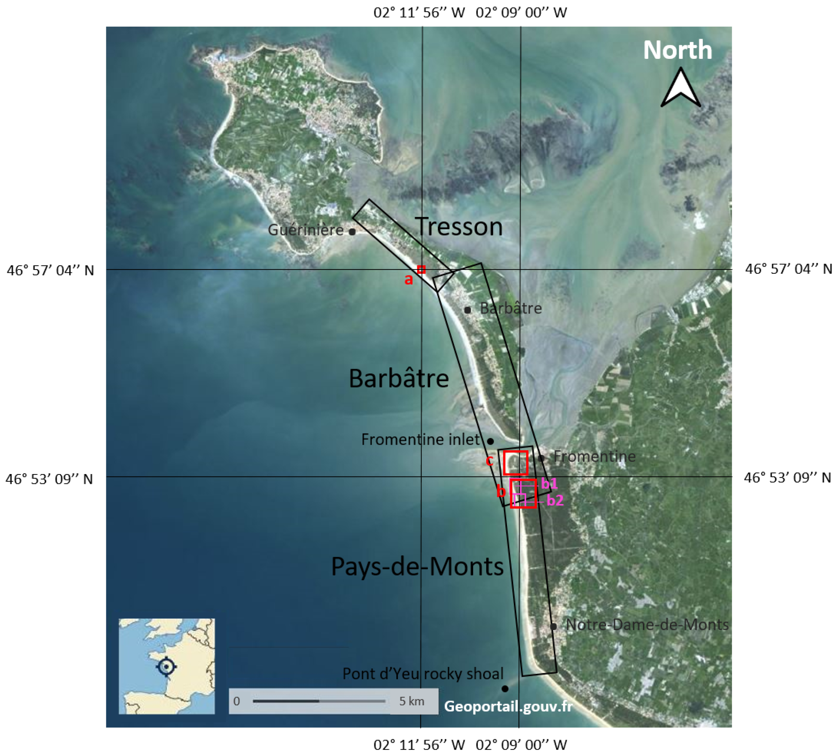
2.1. Study Areas

All the processes of the analysis were established on one training area (presented in Section 2.1.1, see Figure 2). The selected parameters used remain unchanged for the two main validation areas (presented in Section 2.1.2, see Figure 2). For readability purposes, only subset areas are presented in this paper. However, topographical and classification final products were applied to the whole continuous area containing the Tresson, Barbâtre, and Pays-de-Monts beaches (see Figure 2) for the acquisition years of 2017, 2018, and 2019. The corresponding images of the area are available in the Supplementary Materials section.

2.1.1. Training Area: Tresson

Tresson is a rectilinear 1.5 km-long sandy beach located at the southern end of Noirmoutier island’s sandy pit (Figure 2), between the municipalities of Barbâtre and Guériniere. Oriented NW–SE and facing the SW direction, it presents a 8 to 15 m-high dune ridge backed by a large grey dune [63] with a 6 m mean height. It is subject to an alongshore drift toward the SE direction estimated at 25,000 m 3 /year [64], leading to a sediment deficit in the northern part of the spit to the benefit of the southern part. Tresson beach is classified as a “sensitive natural area” [65]. Area a (Figure 2), presented in Figure 2, corresponds to the location of the dGPS field sampling.

2.1.2. Validation Areas

Barbâtre

Barbâtre is a rather rectilinear, 6.5 km-long, sandy beach located at the south of Tresson beach. It is mainly oriented 155 N, facing the WSW direction. Barbâtre beach constitutes the direct continuity of the Tresson one. It follows the same sedimentary flux (SW alongshore drift) on its NW part but is also influenced by the Fromentine inlet forming a narrow tide channel in the south of Noirmoutier island between the Bourgneuf bay and the open Atlantic ocean.

Pays-de-Monts

The north part of Pays-de-Monts is a 8 km-long rectilinear 174 N sandy beach (Figure 2) to the south of the Fromentine inlet and to the north of the Pont d’Yeu rocky shoal of Notre-Dame-de-Monts. The subsidiary areas b and c respectively correspond to Notre-Dame-de-Monts and Barre-de-Monts. Areas b1 and b2 (Figure 2) are locations of the second dGPS field sampling. According to [5], from 1920 to 2010 the coastal morphodynamic of the beach was temporally and spatially heterogeneous and showed a sensitivity to storm intensity and frequency, particularly after the Xynthia storm (2010), which induced a 7 to 8 m coastal retreat. The general current sediment dynamics seems to be a north sediment accretion slowly spreading southward (Notre-Dame-de-Monts).

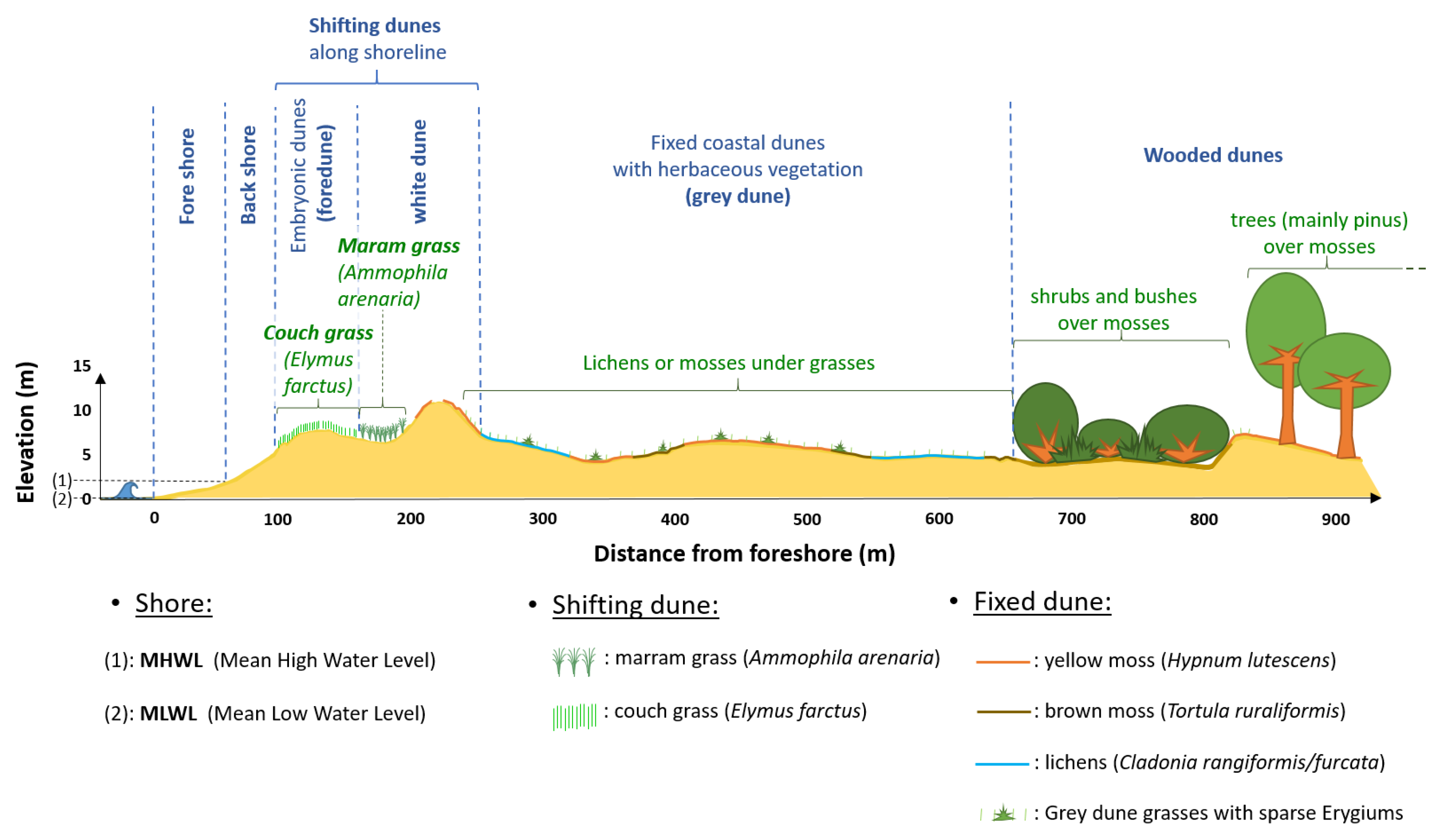
2.1.3. Description of Typical Vegetation Cover

The layout of the sand dune vegetation is mainly controlled by three variables, namely wind, salinity, and sediment mobility. They are all decreasing from the beach to the back-dune. The back part of the dune is mainly defined by its vegetation cover. The wooded part is mainly occupied by maritime pines under which a low vegetation cover is mainly composed of mosses and pine needles. Pines are sporadically replaced by deciduous trees, shrubs and bushy areas. The grey dune, or fixed dune, is mainly composed of a well-established mix, in various proportions, of grasses (mainly fescues: Festuca vasconcensi), mosses (e.g., Tortula ruraliformis (brown moss) and Hypnum lutescens (yellow moss)), a characteristic white lichen (Cladonia rangiformis, Cladonia furcata) locally covered by sparse laguruses (Lagurus Ovatus) with more punctual plants like sea holly (Erygium maritimum), immortal (Helichrysum stoechas) and sea grape (Ephedra distachya). The underlying sand is almost invisible off-trail from the nadir and the spectral variations observed in this area are mainly controlled by the proportion of more or less stacked mosses (brown or yellow), lichens and grasses. The white dune, or mobile dune, is characterized by large areas of nude sand coming off eroded slopes called “caoudeyres” or at the summit along relatively stable pathways, whereas ordinary slopes are mainly covered by sparse low vegetation. In the backward direction, this low vegetation is similar to the grey dune with which it constitutes a transition area, whereas in the forward direction (toward the sea) there is sparse burial-tolerant vegetation. Between the white dune and the foredune, the topography is locally flattened and this is where we find European marram grass (Ammophila arenaria).The foredune, which is in contact with the beach, is mainly covered by couch grass (Elymus farctus) mixed in various proportions with bindweed (Calystegia soldanella) with sparse sea spurge (Euphrobia paralias) over often exposed underlying dry sand. The beach is under the influence tide without vegetation. The top is dry and provides good references of sand reflectance spectra, whereas the low part of the beach is wet and often accompanied by chlorophyllian biofilms.

2.2. Material

The hyperspectral camera used in this study is a push broom Hyspex VNIR 1600, from Norsk Elektro Optikk, Skedsmokorset, Norway. It covers a spectral range from 400 to 980 nm with 3.7 nm sampling and 4.2 nm spectral resolution with a field of view (FOV) of 17 . This camera was used for both airborne acquisitions and vegetation field spectral samplings. Airborne images were also processed with PARametric GEocoding (PARGE) v.3.4 software and the Atmospheric and Topographic Correction (ATCOR-4) v.7.3 software of ReSe Applications LLC, Langeggweg 3, 9500 Wil, Switzerland.
The LiDAR used in this study, which is managed by the Nantes-Rennes university platform, is a Titan dual wavelength LiDAR (green 532 nm and infrared 1064 nm) from Teledyne Optech Incorporated, Vaughan, ON, Canada. A full waveform recorder is plugged only on the 1064 nm infrared channel, which is the most suitable one for topographic and vegetation studies. In order to record the trajectory, it is also equipped with a fast inertia measurement unit (IMU) coupled to the accurate global positioning system (GPS) of POS AV AP50 OEM (IMU-8) from Applanix, ON, Canada.
The differential GPS (dGPS) used in this study is a Leica Viva GNSS, with a GS15 receptor. Measurements were realized in real time kinematic (RTK), enabling us to obtain sub-centimetric accuracy in all three dimensions (x, y, and z).
Finally, bright reference field spectra, serving for the last instrumental noise reduction of the airborne hyperspectral data, were acquired using an ASD FieldSpect3 spectrometer from Malvern Panalytical Ltd., Royston, UK. They can display 2151 bands, which provides a spectral range from 350 to 2500 nm with a 3–10 nm resolution resampled at 1 nm.

2.3. Field Measurements

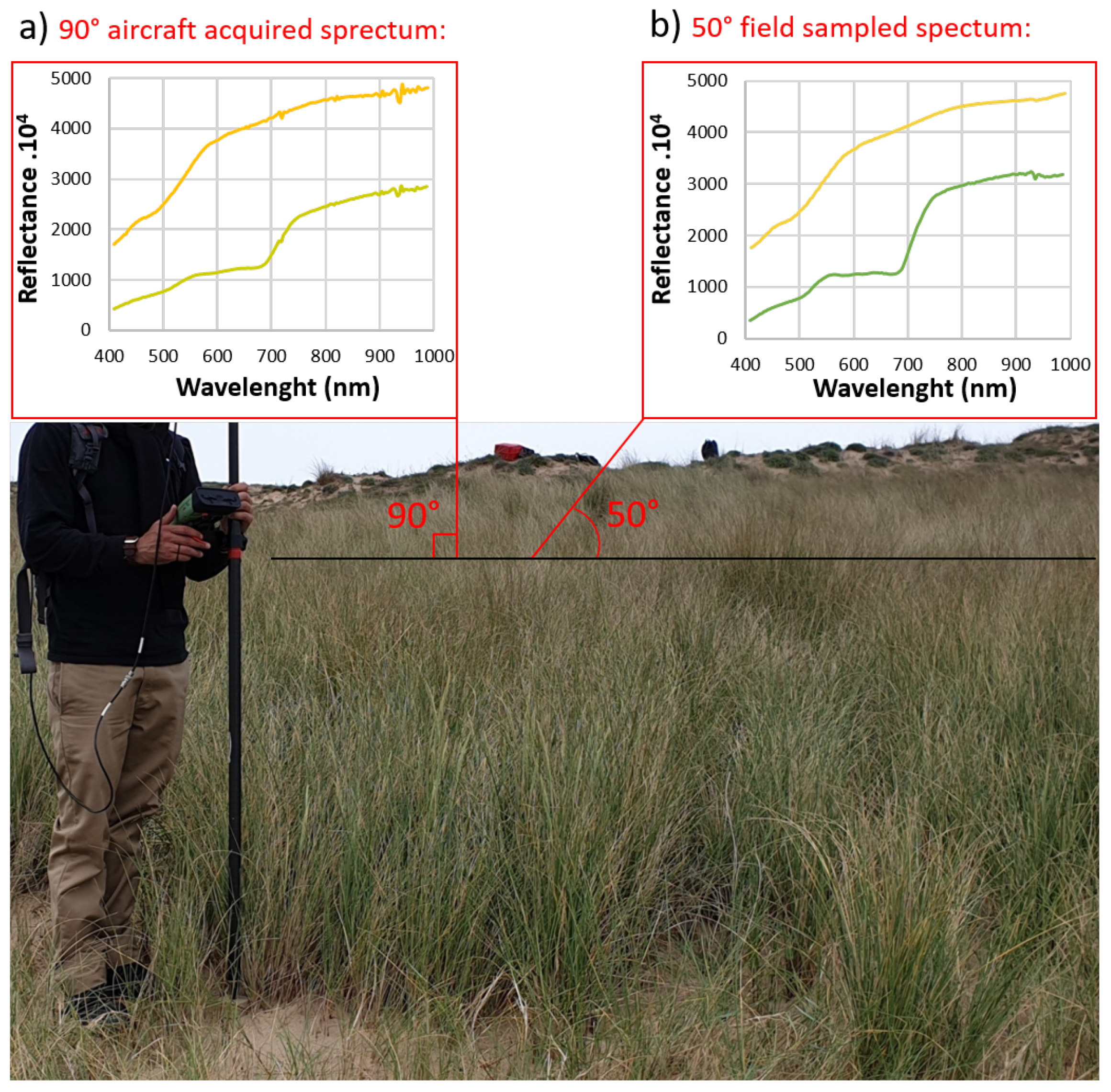
2.3.1. Spectral Field Measurements

In order to demonstrate its ability to extend its application over time, this work reuses the detailed field sampling campaign performed on 16 June 2017 [54]. In order to better understand the spectral properties of the different areas of the dune and find a way to spectrally discriminate their main proxies, a subset of 17 different plants were chosen for their representativeness. To obtain the best match between hyperspectral images, we used the same camera for the 2017 spectral field sampling as in the 2017, 2018, and 2019 airborne campaigns. In the field, the camera was placed on a tripod for panoramic acquisitions acquisitions, thus providing an incident angle of 50 ± 8.5 close to the incident angle of the a sun elevation behind it.
Figure 3 shows a picture taken during an Ammophila arenaria profile of the 2019 dGPS field campaign. Ammophila arenaria’s tufts are greener and homogeneous in their lower part, as their leaves display a rectilinear orientation. However, in their upper part, leaves’ extremities fall in all directions showing no preferential orientation and forming a circular crown of leaves with a bottom–up orientation ranging from 90 to 45 . As both airborne and field images were taken from above, the bidirectional reflection distribution function (BRDF) [66] effects are expected to be similar despite the different acquisition angles but a similar relative angular distribution of leaves. However, the comparison between Figure 3a, displaying the 90 aircraft-acquired Ammophila arenaria mean spectrum taken at 1500 m, with Figure 3b, displaying the 50 field sampled Ammophila arenaria mean spectrum taken at 1 m, shows that these two spectra are not rigorously similar. Indeed, the aircraft spectrum displays a flatter shape than the field one. This is due to the influence of the underlying dry sand always present in the 1 m 2 pixel and masked in the 100 cm 2 oblique close view, which is focuses on the vegetation only. Moreover, as the leaves’ extremities are dryer than their lower parts, the 50 angle of view spectrum contains a bigger proportion of green leaves than the 90 one, which is another factor explaining the differences between these two spectra.
Figure 4a displays the mean spectra of each of the 17 plants that were extracted from ground hyperspectral images using ROIs (regions of interest) constituting the spectral library of the main endmembers of the scene. A few sets of vegetation types are easily distinguishable from the rest. Pines, bushes, and brambles are different due to their green peak of reflectance thanks to their healthy leaves in contrast to all the other yellowing plants. For instance, dry grass, mosses, and lichens display low red-edge. They are characteristically always inclined near an infrared plateau independently of the soil. This has been shown by the ground ROI free of sand. In a grey dune context, at a 1 m 2 pixel scale, the sand is hidden by a thick stack of underlying mosses or lichens covered by grasses and various other plants listed in Figure 4a. They are all intimate mixtures of superposed layers presenting many light interactions between them leading to the definition of a limited number of plant associations spectrally distinguishable from each other, which are: grey dune with an underlying layer dominated by brown and yellow mosses, and grey dune with underlying layer dominated by white lichens spectrally distinguishable from each other.
White dunes and foredunes at a 1 m 2 pixel scale always display a sand surface and appear brighter than grey dunes. Among both foredune proxies, Ammophilia arenaria however presents denser vegetation, which conceals the sand, leading to potentially confusing its spectra with grey dunes. However, both of them, including Elymus farctus, are locally mixed with sedum and other gramineous plants. As a result, the discrimination of these two species is one of the main challenges of this work. Moreover, the multi-temporal classification has to take into account the potential spectral variability of these plants as shown in Figure 4b. Ammophilia arenaria (in magenta) and Elymus farctus (in green) ROIs, which were sampled from ground images, show a strong potential confusion between both grass types. Indeed, each mean spectrum is included in the standard deviation area of the other one, leading to spectral confusion and spectrally-based misclassifications.
Note that in order to remove all remaining defaults after atmospheric correction (detailed in Section 3.2) and insure a perfect matching between airborne and field spectra, ground spectra were acquired over dry sandy beach surfaces for each scene using the ASD field spectroradiometer, as presented in Section 2.2. For each date, the final reference reflectance spectrum resulted from the average of 100 spectra per sample on 10 samples calculated with a Spectralon® and measured in the same geometry.

2.3.2. dGPS Field Measurements

A field sampling campaign was performed on the white mobile dune of Tresson’s training area (Figure 2) in 16 May 2019. A total of 415 position points were recorded using a dGPS (described in Section 2.2). Among these 415 points, 178 were taken on the crest of the white mobile dune, which was stable during the 2017–2019 period, where the ground is nude or only covered by sparse low vegetation. A total of 139 points, which were divided into eight profiles, were taken at the foot of Ammophila arenaria clumps. The latter points will be used to verify the validity of Ammophila arenaria classification results over the training area. In September 2020, a new field campaign, divided into two different parts, was performed: the first part was done on the crest of the white dune of Tresson’s training area, in order to verify its stability from one year to the next by comparing 2019 and 2020 elevation results. A total of 58 points were acquired during this part. However, as the crest line is thin and bordered by slope failures, only 2019–2020 pairs of points, which were separated by less than 30 cm, were taken into account for the stability assessment. As a result, 24 pairs were kept. The second part was performed on Pays-de-Monts validation area c, where 141 points, divided into 10 profiles, were acquired in order to verify the validity of Ammophila arenaria classification results. Among these 141 points, 60 points were on Ammophila arenaria.

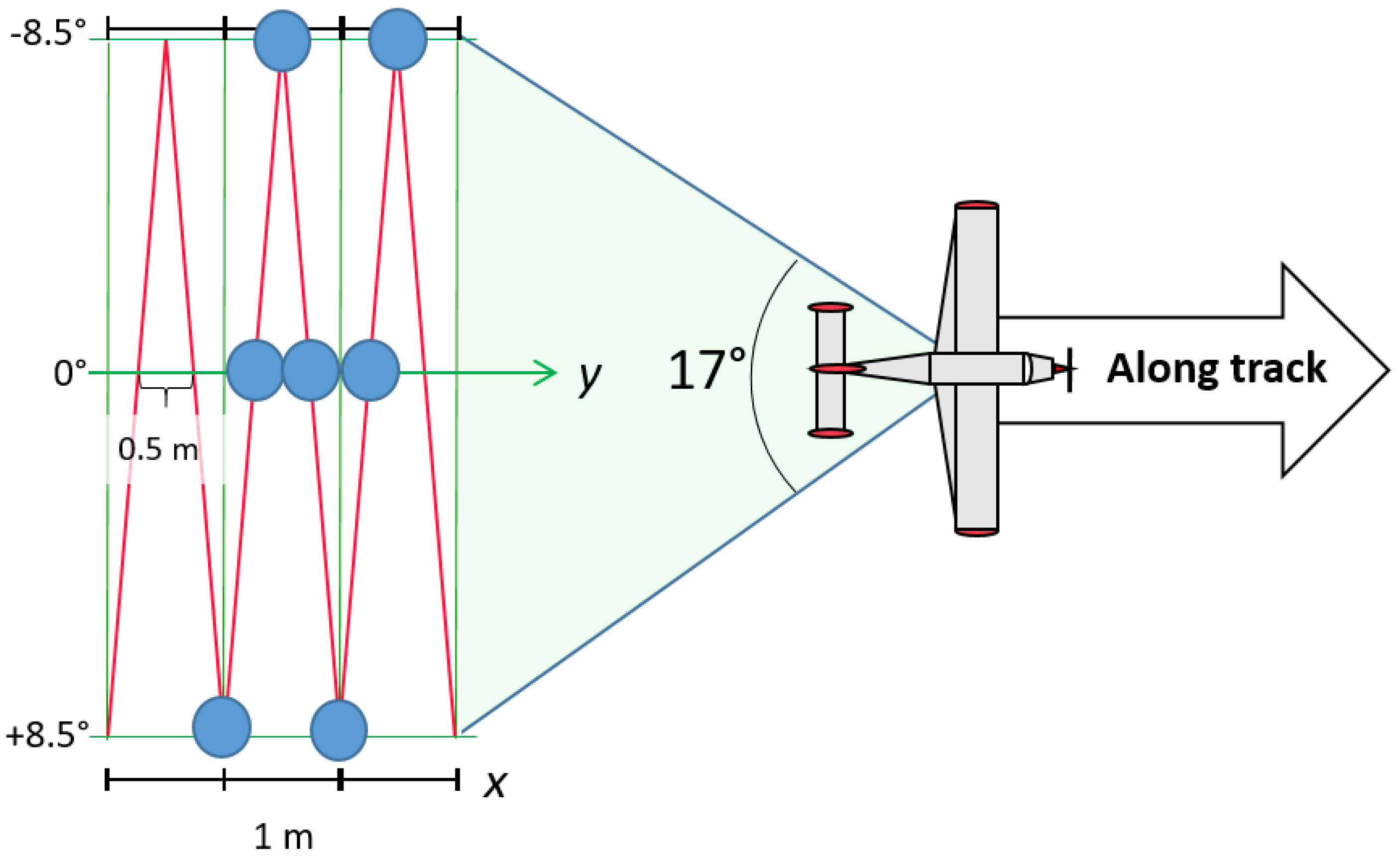
2.4. Airborne Acquisitions

Airborne acquisitions were performed in the context of the OR2C project [67], which is mandated by the region Pays-de-la-Loire to perform an annual coverage of a 250 km-long narrow coastal band susceptible to fast changes. This was performed in cooperation with the GEOFIT-expert and PIXAIR companies with a Chieftain PA31-350 aircraft, manufactured by PIPER, Vero Beach, Florida, United States. In 2017, the acquisitions over Tresson beach were performed on 24 May and both Barbâtre and north Pays-de-Monts dunes were acquired the following day. All areas were acquired on 20 June 2018 and 17 June 2019. Flight lines’ optimization on the sunlight direction, which is ideal for BRDF minimization, were not possible because of budgetary constrains. The orientation of the acquisition flight lines were performed back and forth in polygons following the orientation of the coastline: 115 N for one Gueriniere polygon in 2017 and 2018, whereas there were three in 2019 since they fitted the coastline better. Each year, the Barbâtre polygon is 160 N and Pays-de-Mont one is 174 N. From 2017 to 2019, the airborne above ground level (AGL) was 1500 m at a speed of 240 km/h with a 30% overlap between swaths in order to minimize the risk of having gaps between two lines because of wind gust affecting the plane trajectory. The LiDAR and the hyperspectral camera were positioned one in front of the other to permit the alignment of the VNIR sensor matrix with the 1064 nm laser beam along the same nadir. Despite different incident angles of the light sources (sun and laser), the emergence angles towards the detectors were the same for both types of recorded signals, allowing the LiDAR to follow the same light path from target to sensor.
As the hyperspectral camera has a field of view (FOV) of 17 , it produces a swath width of 448 m from an AGL of 1500 m. Each of the 1600 pixels of the VNR sensor matrix displays an across-track length of 0.28 m. Because of the combination between flight speed and sensor integration time, each row is 0.56 m long along the track. In order to ensure a perfect coverage of the LiDAR scan (red line in Figure 5) over the hyperspectral image, its FOV is set to 17 . Because of this constraint the LiDAR pulse repetition frequency (PRF) was chosen at 175 Hz (150 in 2019) with a scan frequency of 70 Hz to ensure 0.50 m across-track and 0.48 m along-track distances between laser ground footprint centers at the nadir but only a 0.95 m along-track distance on the swath side at plus or minus half of the FOV angle (Figure 5). Considering both AGL at 1500 m and a laser beam divergence pulse width at 0.35 mrad, the footprint diameter is 0.52 m on the ground. Therefore, if all sizes are close to 0.5 m at the nadir, a gap exists on the swath side with a distance of 0.95 m. Consequently, we have chosen to aggregate all data to the maximum resolution size on a single regular grid of square pixels with a size of 1 m across- and along-track. Such a PRF provided a 5.8 pts/m 2 mean point density (5.0 in 2019), which is mainly concentrated along scan lines, as shown in Figure 5, and thus not so well distributed in a 1 m 2 pixel.

3. Methodology

3.1. LiDAR Processing

3.1.1. Discrete LiDAR
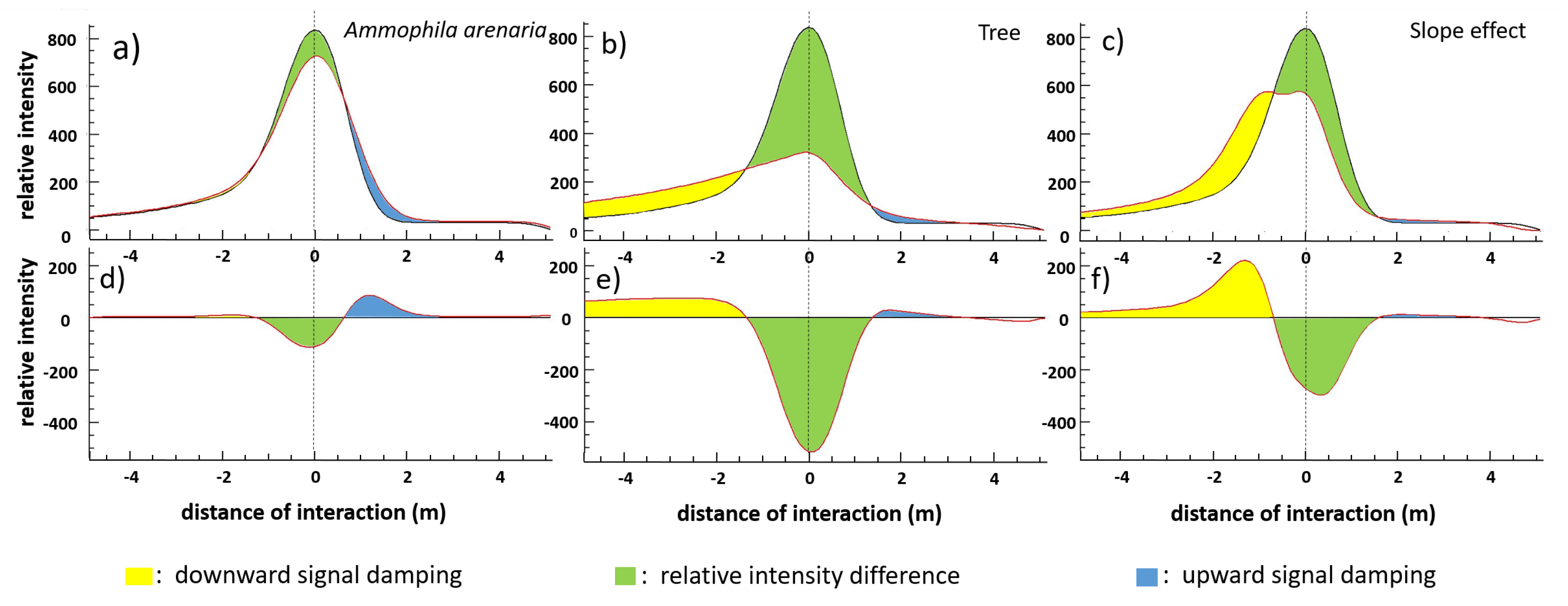
The first and most widely used feature of the LiDAR is the discrete echo. The time of detection of the first echo returned toward the platform gives the range or straight distance between platform and target. The GPS and IMU data records give the trajectory of the plane. The LiDAR Mapping Suite—Professional (LMS) from Teledyne Optech, Vaughan, ON, Canada, 21 November 2018—provides the geographic (x, y) and altitude (z) position of the points with the help of boresighting performed on points overlapping between flight lines [68]. Voids between points are filled by nearest neighbor interpolation in order to produce a raster called the digital surface model (DSM) corresponding to the surface envelope of all points, here performed using ENVI-LiDAR [69], which is also used to classify trees and building to produce the digital terrain model (DTM). These are usually automatically recognized by using classification and segmentation algorithms [70,71] and the underlying ground is approximated by interpolation between the nearest known ground points. However, the vertical accuracy of the LiDAR discrete echo can locally be affected by the presence of complex topography, truncated by interpolation processes, and/or unclassified objects on the ground within the laser footprint [72].

3.1.2. FWF LiDAR

At the discrete echo detection time, the full waveform LiDAR records every nanosecond any intensity greater than a detection threshold chosen by the operator. In practice, the recording of the Titan system starts only at a minimum distance from the predicted ground called the range gate, when echoes are detected to prevent the accumulation of useless signals. The whole backscattered signal is therefore accessible on a length depending on the memory capacity. The identification of a record is given by the traveling time of a laser pulse from its emission to its return time. The energy of a single pulse is spread along a narrow interval of compact material like a roof or soil and a large distance of interaction in case of tree crowns, facilitating the recognition/classification of the corresponding object [52]. In some cases, the backscattered waveform may display several echos, due to the vertical architecture of the considered target that interacted with the laser. In the presence of vegetation, the first one corresponds to the vegetation canopy and the last one to the position of the ground if the laser was able to reach it. Consequently, we have to focus on different echoes in function of the object of interest (canopy, crown or ground/topography). We ensured the perfect coupling of both hyperspectral and FWF LiDAR data on each pixel by projecting the two types of signals onto the same DSM with the same incident angle by using a ray-tracing procedure based on the LiDAR’s GPS and IMU recordings. As discussed by the authors of [54], this procedure permits keeping the whole FWF LiDAR signal along the oblique light path of the hyperspectral data without segmenting it on adjacent pixels induced by orthogonal rectification of a voxelization procedure of orthogonal three-dimensional (3D) cubes [62,73,74,75]. Therefore this ray-tracing method produces a 3D pseudo-cube for each type of data. The first one is the well-known hyperspectral pseudo-cube, containing two spatial dimensions (x and y) and a third wavelength dimension (w) containing reflectance. The second pseudo-cube is the FWF LiDAR one, owning the same two spatial dimensions on a map and a third ranging dimension (r) containing FWF backscattered intensity. Both 3D pseudo-cubes are attached to a 2D map (x, y) of incident angles ( α ) and a 2D map of elevation (z) which is the DSM.
As described in [54], our methodology is based on the relative analysis of slight waveform shape variations. At the wavelength of 1064 nm, all of the vegetation presents high reflectance and the differences are mainly due to chemical compositions, pigment contents and physiological states. In order to focus the analysis on the structure regardless of other variations, it is necessary to use few normalization procedures. Altitude variations are removed by centering the FWF on their first echo (CFWF) allowing to focus the comparison on the relative intensities only at the top of the tree or grass canopy. In this case tree and grass are identified by the thickness of the CFWF. Intensity variations, induced by reflectance and thickness of volume (rising from grass to trees), were removed by normalizing the signal to the maximum of its cumulated histogram (NCFWF) sum of the signal, enabling to focus the analysis on the distribution of the backscattered signal within a given FWF record. The combination of both normalizations is the NCCFWF, from which it is possible to analyze the ranging signature of a given vegetation type. Finally, the derivation of the NCCFWF, called dNCCFWF, permits coming back to the usual pseudo-Gaussian shape of the FWF signal, without altitude, intensity, and amplitude effects.
In detail, the recording of the FWF signal is activated by the detection of the first echo of the back-scattered signal, initiating a recording sequence of 60 samples limited to a sampling period of 1 ns corresponding to a 15 cm range [50,76]. As the footprint diameter is about 0.5 m with a point density of 5 pts/m 2 for a pixel resolution of 1 m 2 pixels (Section 2.4), several waveforms are stacked in a given pixel. Figure 6a presents the 15 cm resolution raw FWF signal of three key surfaces: beach dry sand, Ammophila arenaria, and white dune steep slope. Figure 6b represents the result (dNCCFWF) after using a cumulative low pass filter defined by [54], which is necessary for noise reduction. The corresponding image (Figure 6c) shows that Ammophila arenaria and white dune steep slope effects remain too close to each other with an aliasing that is well visible in the image due to the 15 cm bin digitization of the FWF range. Figure 6d shows that the simple application of a classical median filter [77] to each range channel (along the r dimension) reveals sub-pixellar information. Subtle variations caused by atmospheric scattering produce a jagged laser beam path, which induces noise by moving it in a tiny neighborhood, defocusing the signal. The selection of the best intensity found in a small neighborhood was efficient to refocus the signal and retrieve the 0.5 m footprint signal within a 1 m 2 pixel. However, as shown in Figure 6e, the following low pass smoothing procedure tends to erase a part of the sub-pixellar information without removing the aliasing effect that is also well visible in Figure 6f. Knowing that each FWF record starts at a distance set for each pulse, two consecutive pulses can fall by ray tracing in the same 1 m 2 pixel but at two different lengths of the ground (in the case of sloppy ground for instance) and not always in the same 15 cm bin of a pseudo-cube.
Figure 6g illustrates the stacking procedure at 5 cm. Dune slope areas are two consecutive FWFs recorded with a 15 cm resolution from different initial elevations, resulting in a vertically offset (not aligned) resampled at the vertical resolution of 5 cm. As shown in the Figure 6h–j, the vertical resolution set to 5 cm, without range median filtering, only removes the aliasing effect. The median filter cleaning procedure (Figure 6k) remains necessary to remove the atmospheric scattering effect and focus the signal (Figure 6l). Thanks to the 5 cm vertical resolution, the filtering can be three times narrower, which leads to a perfect distinction between both Ammophila arenaria and steep slopes (Figure 6l) enhanced by the first echo CFWF procedure, without having the 15 cm aliasing effect with well-contrasted colors in the color composite image (Figure 6m).
As the dry sand is the best backscattering material of the studied scenes, inducing no specular reflection as defined by [66,78], the full-waveform resulting from its backscattering is close but not identical to the emitted waveform, making it perfect to be used as a reference for a relative comparison procedure [54,79,80]. Figure 7a–c show the relative comparison between the dry sand dNCCFWF and three major objects of the scene. The deformation induced by these objects on the FWF signal becomes easier to catch when each dNCCFWF pixel is subtracted by a dry sand dNCCFWF reference (Figure 7d–f). This permits to simply define a rule of straightforward classification of low vegetation like Ammophila arenaria and other grasses presenting the same distribution of leaves scattering the FWF, therefore requiring some complementary information discussed in the next section. The FWF analysis is summarized in indices facilitating their combination with hyperspectral ones. Both indices are areas calculated on a short interval at −0.5 and +2.5 m of the dNCCFWF centering range set to 22.48 m for the analysis of longer patterns of FWF distortion, such as trees partially shown here (yellow in Figure 7).
The first one, noted as FWF down, is a fraction of the dNCCFWF area (green in Figure 7d–f), taken in the −0.5 to +2.5 m interval. It is used here to show that the analysis of the top of the canopy can be sufficient to distinguish trees from bushes without analyzing the full thickness of that vegetation. The second one, noted as FWF marram, is the dNCCFWF area departure from the sand (blue in Figure 7d–f), which is conditioned (Figure 7d) to an intensity greater than −200 at the dNCCFWF center (compared with Figure 7e,f). Both indices are stored in a map facilitating their combination with hyperspectral data for final classification.

3.2. Hyperspectral Processing

The recording of aircraft attitude, using the GPS and IMU associated with the LiDAR, allowed the GEOFIT-expert company to calculate the trajectory. From this trajectory, it was possible to correct the geometry of the hyperspectral raw data by using a ray-tracing procedure that projects a vector from the aircraft position, using dGPS records, following the angles recorded by the IMU, which allows to locate the pixel of interest at the intersection point between the vector and the plan displayed by the LiDAR DSM [81]. This procedure was performed using PARGE software [82]. A second order of geometric correction using ground control points (GCPs) is often necessary in order to guaranty a sub-metric horizontal accuracy. Atmospheric corrections were then performed using ATCOR software [82]. The latter uses the MODTRAN5 atmospheric model enabling to estimate for each pixel the water vapor content, based on the 820 nm channel, and the aerosol diffusion effects [82]. Here we chose to use a maritime (coastline not fully oceanic) atmospheric aerosols model. The acquisition dates and times (given the sun elevation) were taken into account as well as recording angles, provided by PARGE output files. After the geometric and atmospheric corrections, the different acquisition lines were assembled. Then a minimum noise fraction (MNF) transformation [83] was applied. The first 15 MNF bands were selected for the MNF inverse transformation. Finally, an adjustment on a bright target was performed in order to remove any instrument artifacts that could not be statistically identified by the MNF. This procedure, which insures the best matching between airborne and field instruments, was performed by using a single bright dry sandy reference made of 100 spectra collected on the ground with the ASD spectrometer divided by its ROI in the image.

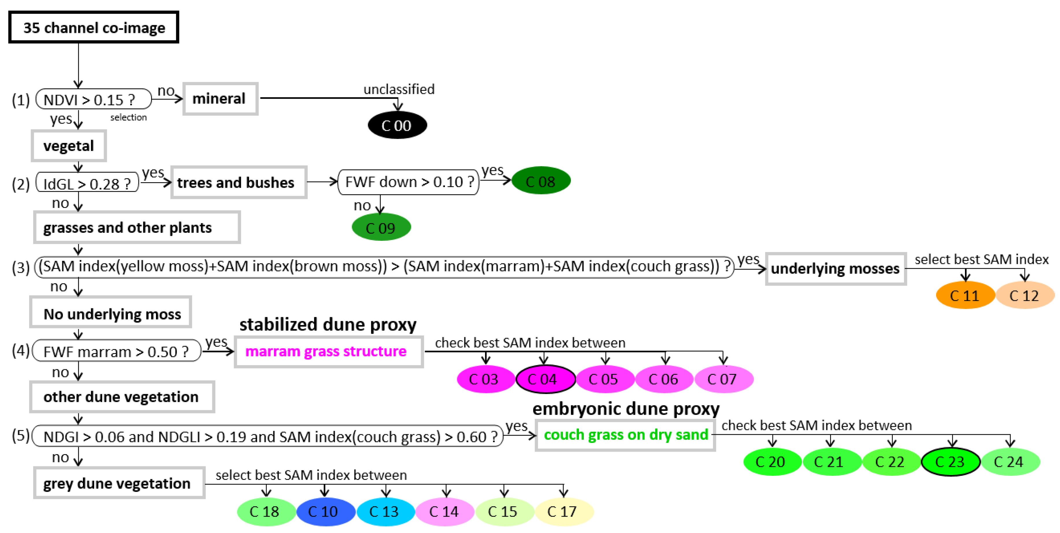
3.3. Classification of Main Dune Vegetation Proxy

3.3.1. Straightforward Hierarchical Classification of Dune Proxies by Combination of FWF and HSI Data

In this study we aimed to quickly sort all main components of the image in order to focus the analysis on the vegetation proxies of the dune dynamics. This is done on a co-image gathered in a 35-channel image, the collection of maps of indices predetermining a distance of classification to a class defined either on hyperspectral or LiDAR data. These are two or three-band hyperspectral indices defined by the authors of [84] as follows: “a spectral index is a number qualifying the intensity of a phenomenon which is too complex to be decomposed into known parameters”. Many of them are summarized in [84,85]. The aim of the famous normalized difference vegetation index (NDVI) [85,86,87,88], rewritten at HySpex VNIR resolution [48], was to minimize the shadowing effect between slopes on relief like dunes, for example. However, because of common effects of BRDF on leaves, depending on combinations of sun elevation, flight line direction, and effective local emergent angles, unexpected variations may occur between images’ sides. Thus, threshold values are only used for the basic segmentation of large vegetation groups. Following the NDVI model, we defined other indices, designed for HySpex bands (Table 1), to evaluate the NIR slope of the vegetation plateau for a grass index (Normalized Difference Grass Index, NDGI), identify the narrow slope of the reflectance peaks in green (Normalzed Difference Green Leaves Index, NDGLI) and red (Normalzed Difference Red Leaves Index, NDRLI) leaves’ indices, and use three bands to fully outline those green (Index of Green Leaves, IdGL) and red (Index of Red Leaves, IdRL) peaks [89]. The full resolution of hyperspectral images leads to directly recognizing the chemical components in a reflectance, making more accurate classifications. However, many vegetation types have the same chemical composition and one reflectance spectrum may correspond to many different vegetation types. Despite this, it is possible to use one reflectance spectrum as a descriptor of the information contained in an image. A perfect match between image and reference spectra never guarantees the identification of a plant. It can attest to its resemblance and combining this with other parameters can finally converge toward a solution. Like the NDVI, the spectral angle mapping (SAM) [46,90] was first defined for shadow effects’ minimization with the help of the angular distance between reflectance spectra seen as long (bright) or short (dark) vectors that are insensitive to lighting intensity variations. Like the NDVI [87], SAM angles are sensitive to seasonal and directional variations between two or more acquisition dates. It is however possible to minimize the effect by ranking SAM angles within each image, as discussed in [91]. Instead of trying to define multiple angular thresholds of classification, which would change from one date to another, a ranking between the SAM angle to series of reference spectra allows to set a hierarchic classification on moving conditions of image acquisitions. However, the comparison between parameters varying in too different magnitudes would always fall on the boundary between such strong gaps of intensities. This could be the case when comparing SAM angles with dimensionless hyperspectral indices. This is avoided by the use of the SAM index (Table 1) ranging from 5 to 1000 for poor to perfect matching, respectively, instead of SAM angles ranging from 200 to 0 mrad, respectively, whereas irrelevant data are limited to a range of 0 to 5 instead of 1000 to 200 mrad [48].
First, a well-known NDVI [85,86,87,88] rewritten at HySpex VNIR 1600 resolution [48], enables setting apart non-vegetation pixels in the class C00, which would not be considered by the classification. The threshold of 0.15 is the value of the NDVI of dry sand without any vegetation cover. As noticed in Section 3.1.1, all trees (pines, oaks), shrubs, and bushes displaying green peaks of reflectance with a tight red-edge and a low rising NIR plateau are easily set apart with the three-band IdGL index (Table 1). Then, they are segmented into two main classes based on FWF information, presenting a long downward backscattering (>0.10) for trees (C08) and short one for shrubs and bushes (C09), which will not be further analyzed in this study. Following the same analysis of field reflectance for the grey dune, all of the areas dominated by underlying mosses are easily segmented by ranking SAM indices of mosses with SAM indices of marram and couch grass. Grey dunes were eventually segmented into C11 (yellow moss) or C12 (brown moss) classes using the internal ranking of their SAM indices. At this stage, Ammophila arenaria is readily segmented by a threshold of the FWF marram index. Nevertheless, a SAM index relative comparison procedure allows to analyze the variable spectral proximity of Ammophila arenaria to grey dune grasses (C03), itself (C04), fescue (C05), couch grass (C06), and straw mixed with dry sand (C07), which will be analyzed in the results section. As a permanent sand background characterizes the foredune proxy, Elymus farctus, its discrimination is possible thanks to the combination of the Elymus farctus SAM index with the NDGLI and NDGI indices. Once again, a SAM index relative comparison procedure permits the analysis of the variable spectral proximity of Elymus farctus to grey dune grasses (C20), Ammophila arenaria (C21), fescue (C22), itself (C23), and straw mixed with sand (C24), analyzed in the application section. Finally, remaining pixels correspond to the grey dune vegetation and other foredune vegetation, which are classified using the direct SAM index ranking, allowing to map grey dune lichens (C10), other herbaceous plants with lichens (C13), Ammophila arenaria (C14), Festuca (C15) Elymus farctus, (C18) and straw mixed with sand (C17).
Once we obtained the classification results, and in order to reduce the salt and pepper effect and have more spatially homogeneous classes, we slightly smoothed the classification. To do this, we applied a majority 3 filter, proposed by ENVI, which consists on a 3 × 3 pixels structural element attributing to the central pixel the value of the majority of the nine considered ones [77]. In order to verify the quality of the classification results, the latter will be compared to field measurements. For the working area of Tresson the classification results will be compared to dGPS field measurements performed over Ammophila arenaria.
In Section 4, only the three main vegetation proxies (Ammophila classes C3–7, Elymus classes C20–24, and sparse vegetation over dry sand classed as C17) will be presented over the subset areas presented in Section 2.1. However, the whole classification results are available in the Supplementary Materials: S1 and S2 respectively display 2018 and 2019 classification results (2017 displayed no significant differences with the 2018 results).

3.3.2. Classification Validity Assessment

In order to assess how accurate the classification results are, dGPS field measurements, acquired over the Tresson beach training area and the Notre-Dame-de-Monts validation area c (see Section 2.3.2), was compared to the polygons resulting from the classification. Of dGPS points having located Ammophila arenaria on the field, those that correspond to pixels classified as Ammophila arenaria were used to determine the “perfect matching” percentage. Another matching percentage, taking into account a one-pixel width buffer zone around the classification polygons, was calculated to integrate the signal dilution effects occurring at the edges of the region of interests.
As discussed in Section 2.3, Ammophila arenaria (class C4) can display spectral signatures similar to Elymus farctus (class C6), but also to the fescue (Festuca vasconcensi, class C5) and other types of grasses of the dune (C3). Note that all of these classes (C3–7) are classified as Ammophila arenarie based on FWF LiDAR telemetric information, but they differ in their spectral proximity. Considering the spectral variability of these plants and a spectral library of reference spectra acquired on the field in 2017, a dune vegetation proxy classification only based on spectral information would not be possible. This is the reason why we also used the FWF LiDAR ranging information. As a validation, a spectral proximity test was performed on pixels classified as Ammophila arenaria (C3–7) to assess the percentage of spectrally closest pixels to other reference spectra. The same test was also performed on Elymus farctus classified pixels (C20–24). The results are available in the Supplementary Materials (see S3) but not discussed in this article, as these classes were not discriminated from FWF LiDAR information.

3.4. Topographic Analysis Methodology

The comparison between airborne LiDAR and ground dGPS elevation values was performed over different areas. The white dune crests are sand paths only covered by sparse vegetation and morphodynamically one of the most stable areas, which is convenient for local high precision calibration.
In 2003, the French Institut Geographique National (IGN) and Service Hydrographique et Oceanographique de la Marine (SHOM) were instructed by the French authorities to produce together a topographic and bathymetric model of French coasts [92]. This idea aimed to create a unique database available for all coastal managers. These data are mainly LiDAR DTMs, acquired every 10 years along all French coastlines with a standard spatial resolution of 1 m [93,94]. OR2C permits an annual sampling of the different processes impacting the coastal morphodynamics, in complementarity with the decennial IGN’s Litto3D studies. In Pays-de-la-Loire, Litto3D data are available in 2010 and 2019 for the closest comparison with our 2017 to 2019 data. The closest 2019 Litto3D data were acquired between the 2nd and the 3rd of February 2019. The 2010 data, containing significant tracks of the Xynthia storm [95], were also included in this work.
According to [96], the overall morphodynamics of regional sandy beach foredunes can be performed in a 150 to 300 m buffer zone from the altitude zero line, which explains the restriction of the analysis to this area. The areas covered by dense Ammophila arenaria (C4) clumps being investigated for their impact on airborne LiDAR topography and the polygons of the classes C3 to C7 (Figure 8) were used to define a more restrictive area of analysis.
As for the classification results, topographic results will be presented in Section 4 over the subset areas presented in Section 2.1. However, applications to the whole areas are available in the Supplementary Materials as S4 and S5 respectively for the 2018 and 2019 acquisition years (2017 is not provided as it displays no significant differences to the 2018 results).

4. Results

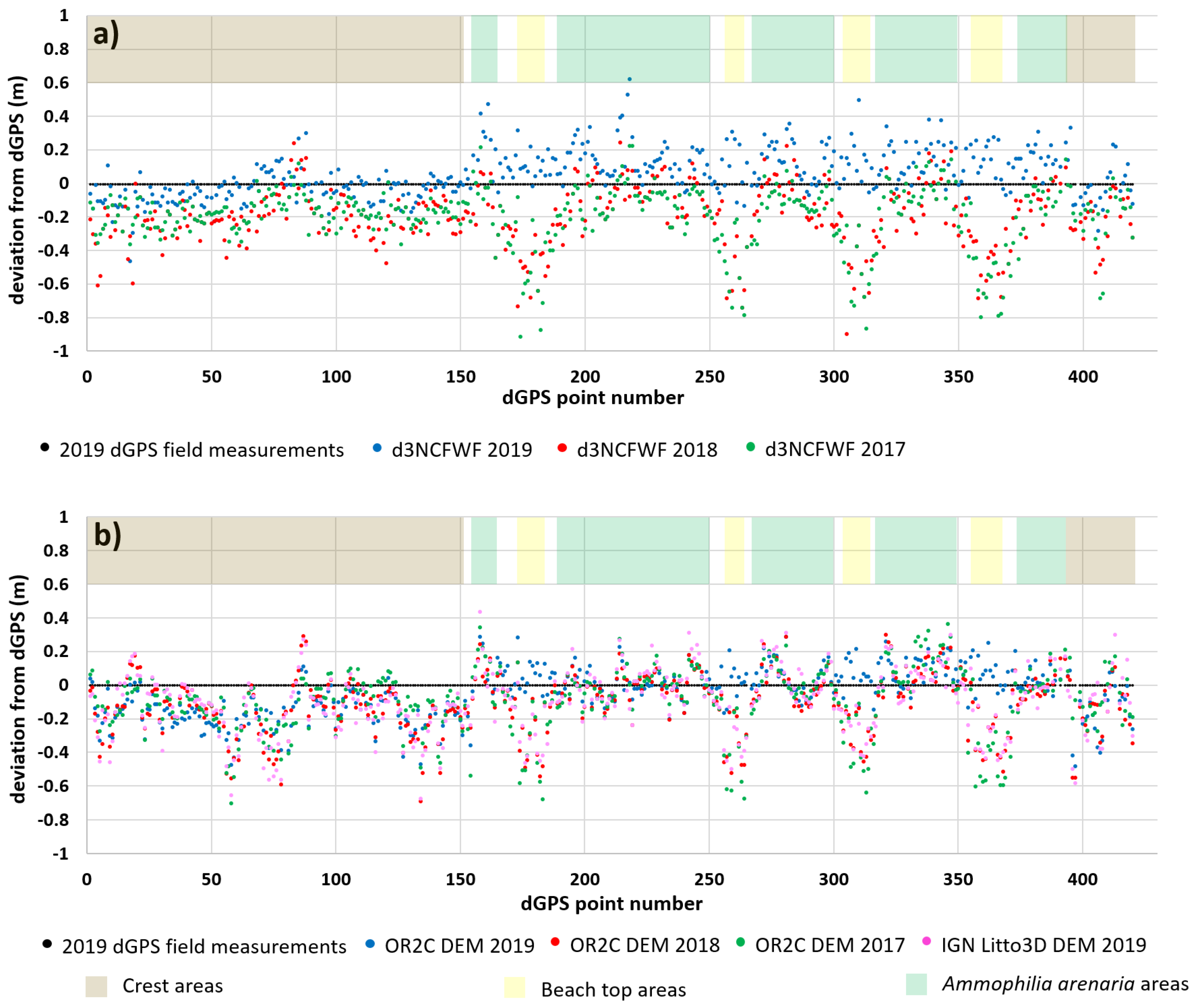
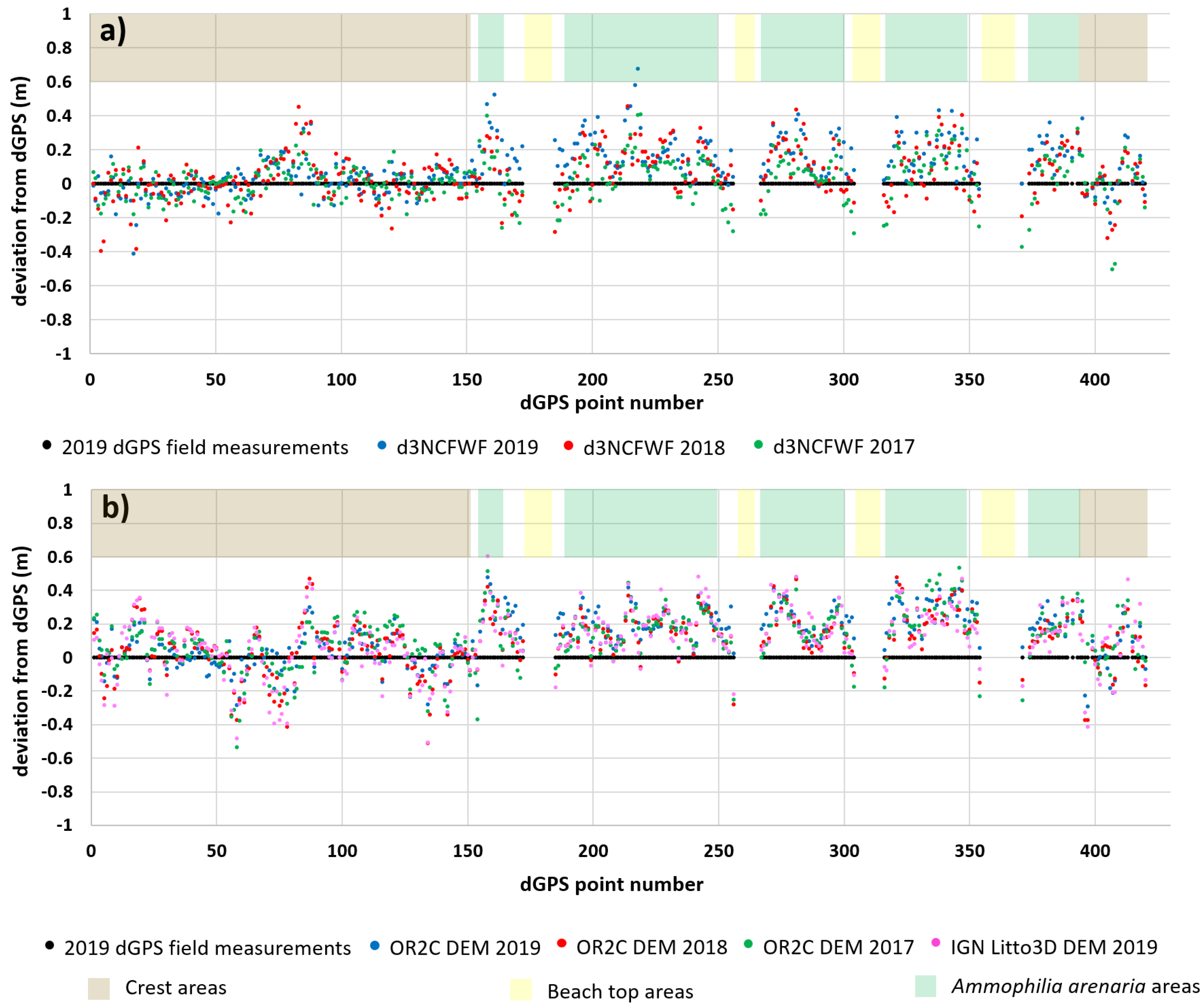
4.1. Topographic Analysis: Comparison between LiDAR Data and dGPS Field Measurements
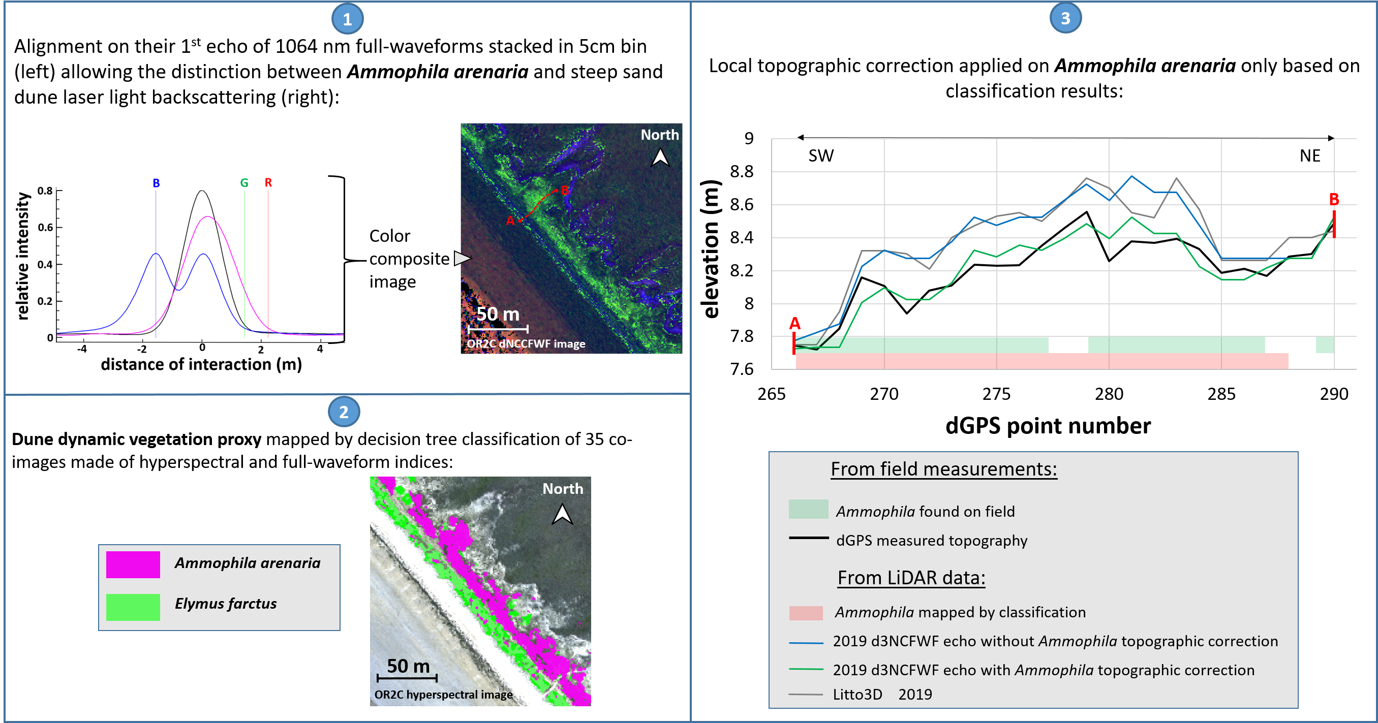
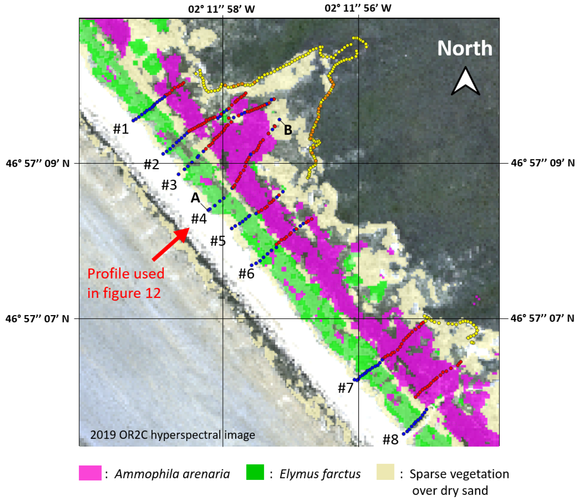
The comparison between the 2019 and 2020 white dune crest dGPS field samplings shows a 0.01 m mean deviation and a 0.028 m RMSE, showing that the dune is stable enough to be taken as a calibration reference for the 2017–2019 data.
The analysis of the LiDAR signal deviation over the points located on the reference white dune crest (brown areas in Figure 9) shows a mean underestimation of the elevation of −0.22 m with a 0.10 m standard deviation in 2018 (like in 2017). In 2019, after a new factory calibration, the average deviation was reduced to −0.04 m with a 0.10 m standard deviation.
At the locations of Ammophila arenaria clumps (green areas in Figure 9), the mean deviation was 0.20 m ± 0.27 m for both 2017–2018 and 0.06 m ± 0.15 m in 2019. The period of 2017–2018 displayed better apparent results because of height compensation of their ground elevation evidenced on the white dune crest. It was therefore necessary to first calibrate the airborne LiDAR signal in order to focus the analysis on the Ammophila arenaria clumps’ effect alone, which is done in Figure 10. The first echoes of the d3NCFWF of Figure 9a are more scattered than the pixels of the discrete DTM in Figure 9b but both show the same trend of elevation underestimation compensated in marram grass areas. The embryo dune bottom and beach top (yellow areas in Figure 9) were not used in the calibration because of strong variation between dates.
For high precision analysis on local dGPS GCP, the mean deviations giving the calibration factors were calculated over crest areas and were +0.177, +0.216, and +0.038 m, respectively, for 2017, 2018, and 2019 airborne LiDAR elevations (Figure 10). Beach top values, located under 7 m elevation, have been removed. Moreover, 13 points were removed from the 178 calibration crest points dataset because of inducing second echos, meaning that they were located on sloppy pixels, which is not acceptable for a calibration reference area. Airborne LiDAR mean deviation has been reduced almost to zero on the ground, which emphasizes the idea that both d3NCFWF signals and discrete echoes show a positive deviation over Ammophila arenaria areas. This confirms that Ammophila arenaria clumps do not allow the LiDAR signal to fully penetrate the vegetation width to the underlying ground. This overestimation of the ground elevation reached its maximum around 25 cm in the middle of marram grass spots and decreased at edges, where it became negligible. Surprisingly, in top crests free of marram grass, the RMSE of d3NCFWF ground elevations were 0.10, 0.13, and 0.10 m, respectively, for 2017, 2018, and 2019. These RMSE are smaller than those of the discrete DTM with 0.17, 0.14, and 0.12 m, respectively, for 2017, 2018, and 2019. This effect, which reached 0.3 m in narrow locations, was induced by the discrete echo neighboring interpolation process used to build the DTM while d3NCFWF echoes are always processed at the pixel size. The 1 m 2 pixel-based calculation of d3NCFWF is therefore suitable to better follow the detailed morphology of the ground.
In order to guarantee an optimal elevation model quality, it was necessary to isolate Ammophila arenaria’s areas to correct them independently from the rest of the scene.

4.2. Training Area

4.2.1. Ammophila arenaria Selection by FWF

The polygons corresponding to the Ammophila arenaria classification in Figure 8 are represented in magenta areas with dGPS field measurements in red points in Figure 11; green areas are couch grass and blue points are other vegetation covers including Elymus farctus. A total of 73.3% of Ammophila arenaria field sample points corresponded to pixels. They have been successfully classified as Ammophila arenaria (magenta areas/red points in Figure 11). However, considering a 1-pixel uncertainty width buffer zone around the resulting polygon, because of the use of a majority filter of classification results, the score reached 90.9%. As Elymus farctus is an important proxy of the foredune it was important to select it but this has no impact on topography.
In detail, Table 2 shows that only a fraction of the marram grass observed in the field spectrally matched with Ammophila arenaria (class C4) and that it was often spectrally closer to Elymus farctus (class C6). C7 is a class of sparsely vegetated over-exposed dry sand that could belong to both of them. C5 is festuca and C3 is other grass types on the dune. As stated in Figure 4b, a pure hyperspectral classification could not segment both vegetation proxies and FWF data are absolutely necessary in this case. However, the hyperspectral data confirmed the domination of the spectra by marram and couch grass, which could not be done by FWF alone, which confirms the complementarity of both techniques. All other vegetation types presenting too small SAM indices were not studied in both vegetation proxies, which also confirms that hyperspectral methods can provide standalone diagnostics of vegetation groups.

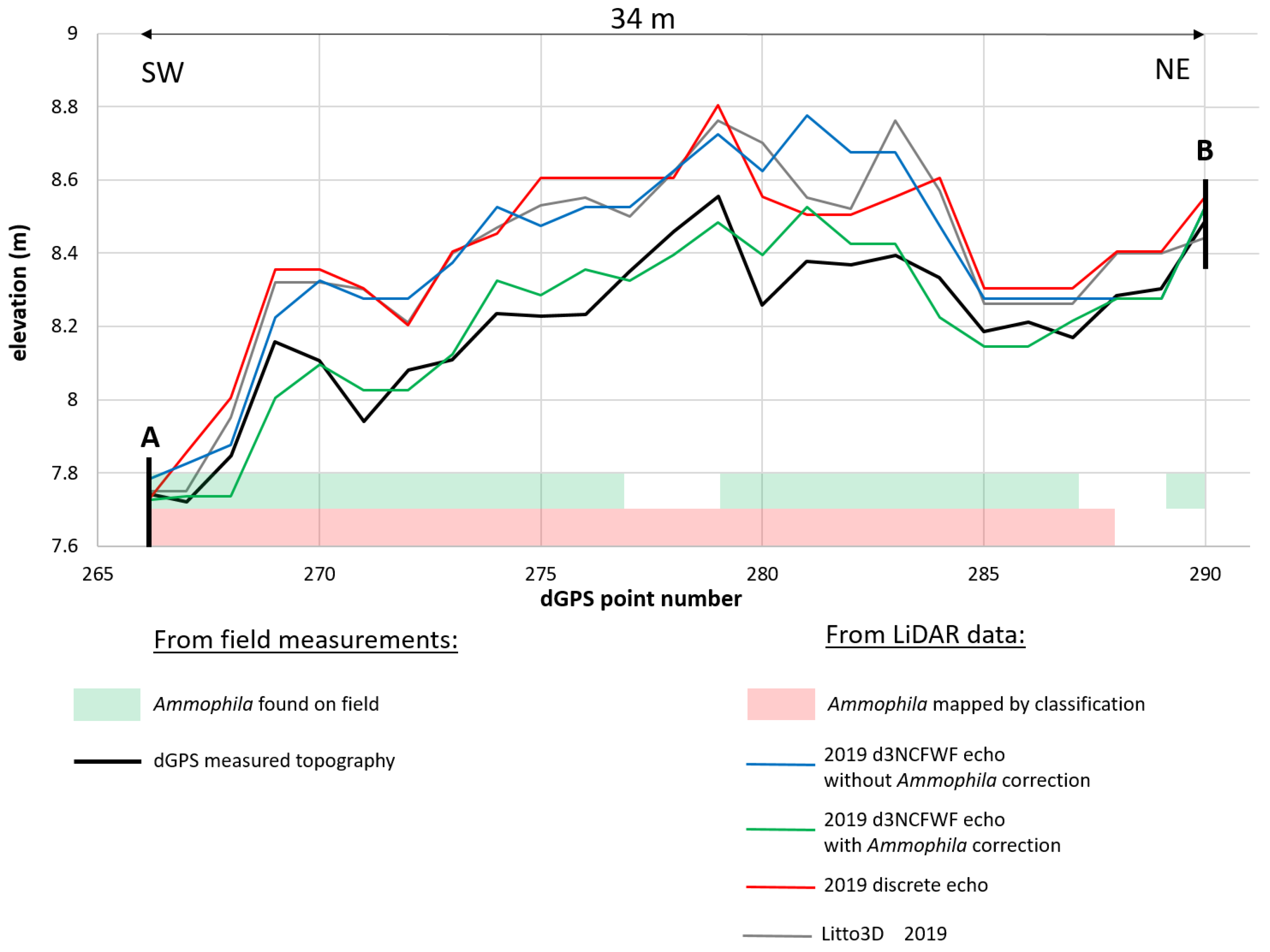
4.2.2. Ammophila arenaria Topographic Correction

Unfortunately, we could not find a valid estimation of the vegetation height in each pixel. It seems that the dNCCFWF (Figure 7a) can only detect a bulk deviation of 0.25 m from the topography without any probative correlation to the effective length of the leaves measured in the field. This would require the analysis of higher vegetation occupying more than one or two bins of the FWF record. Consequently, we decided to apply a correction factor of 0.25 m, corresponding to the average deviation induced by Ammophila arenaria evidenced in Figure 10. The application of a 5 by 5 pixels low-pass filter to this constant correction factor allows simulating its decreasing effect on the edges. Figure 12 presents the topographic profile 4 (Figure 11) as an example. While the black line corresponds to the ground dGPS reference, the blue line corresponds to the original 2019 FWF echo topography, and the green one is corrected with the 0.25 m plus 5 × 5 low-pass procedure applied on Ammophila areas only. The 2019 Litto3D IGN reference, which is also aligned with dGPS data for local high precision analysis, is grey, and the red line corresponds to the discrete last echo. Ammophila arenaria did not induce several echoes and the signal was not able to fully penetrate the vegetation width to the ground. Consequently, first or last echoes would provide the same results. The analysis of the deviation from the dGPS field measurements over Ammophila arenaria sites showed a reduction of the RMSE from 0.24 to 0.13 m for 2019 and from 0.20 to 0.12 m for 2018 data. In comparison, the IGN Litto3D displayed, without marram grass correction, an average error of 0.20 m over these points.
Note that all elevations, including IGN ones, are provided on a kilometric map with a precision of 0.30 m. Any local high precision requires alignment on GCPs. In absence of close standard GCPs, refining procedures with dGPS acquisition are required.
Figure 13 presents the full Tresson’s training area with the application in the coastline buffer. It combines topographic and classification results for both 2018 and 2019 (2017 is not presented because of no noticeable difference with 2018). In 2018 (and by extension, in 2017, which not presented here), both the Ammophila arenaria and Elymus farctus classes’ surface increased from the NW to the SE. In the NW, Elymus farctus presents a local inland extension that is reduced to a narrow foredune edge along sparse marram grass implantation. Note the presence, in 2018, of an Elymus farctus patch in the NW extremity of the white dune crest, which almost disappeared in 2019, indicating the digging of a blowout basin during this period. In the SW, both proxies are well implanted in large and compact bands, testifying to feeding dynamics in contrast with narrow bands of the NW in erosion. This observation is in agreement with the SE-ward sediment drift. In 2019, the extension of the Elymus farctus implantation shows that the foredune, which was not there in 2018, is rebuilding. Moreover, the southern area followed the same dynamics with increasing widths of both Ammophila arenaria and Elymus farctus.
The topographic profile, presented in Figure 13c, has been chosen on the northern part of Tresson beach and the white dune. The OR2C data, either from FWF or discrete echo detection, show a beach-top accretion from 2018 to 2019. The foredune has been remarkably stable and a slight erosion has affected the white dune crest. The 2010 Litto3D shows the level of the beach after Xynthia, which led to an important erosion of the beach and the foredune. The comparison between 2010 Litto3D and 2017–2019 elevations highlights the resilience that occurred in this amount of time.

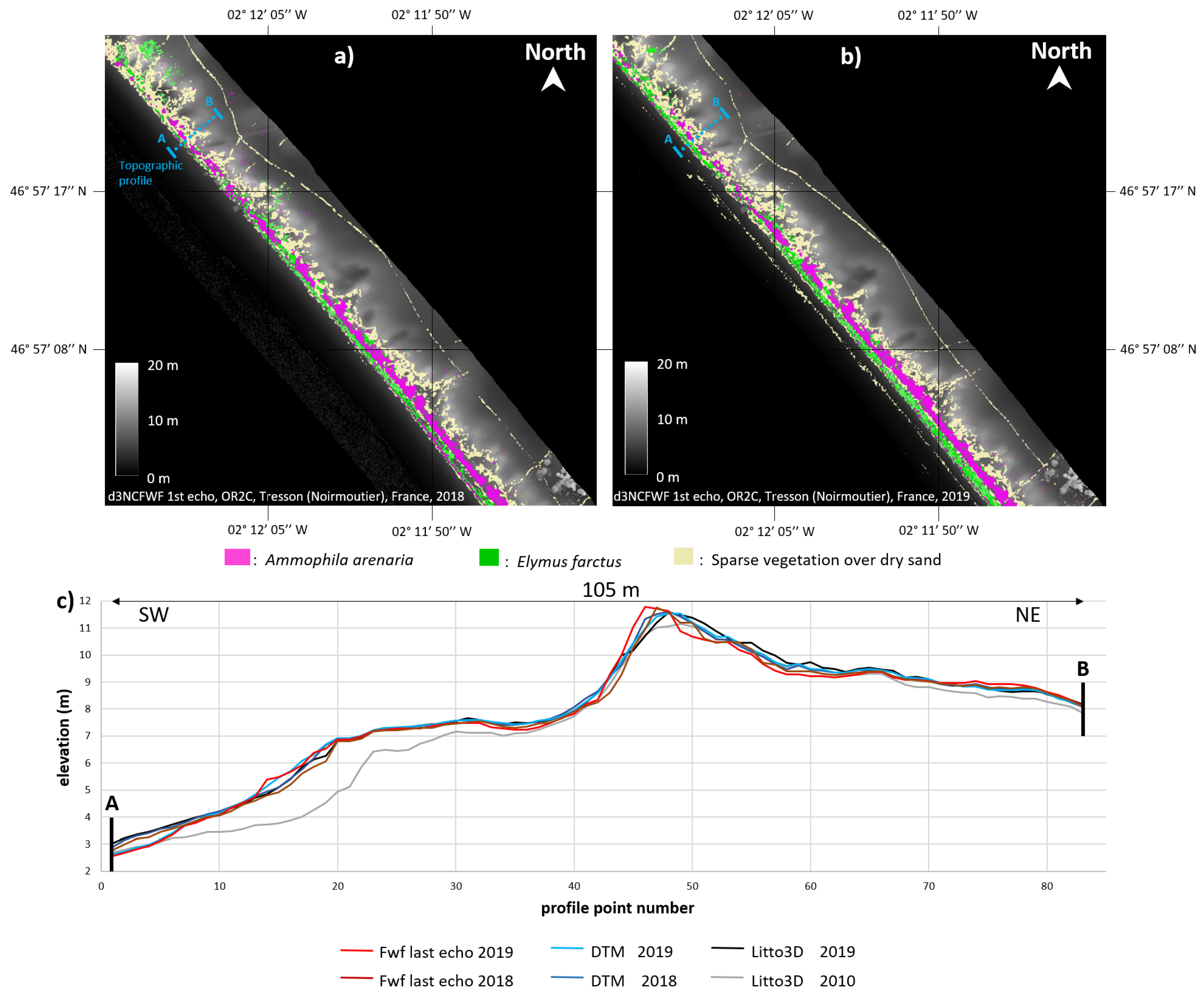
4.3. Validation Area

4.3.1. Notre-Dame-de-Monts

The full area is presented in the Appendix (see location in Figure 2); only two subsidiary areas, b and c, are presented at a printable magnification. The classification implemented on the Tresson training area was directly applied to north Pays-de-Monts (see location in Figure 2) without any prior knowledge of Ammophila arenaria (magenta in Figure 14a) and Elymus farctus (green in Figure 14a) locations. Figure 14 shows field dGPS points acquired on Ammophila arenaria areas in red, other foredune vegetations in blue, and beach-top sand in yellow. The profiles acquired in 2020 cutting 2019 Ammophila arenaria (magenta) polygons larger than 3 pixels (Figure 14a) display a perfect matching percentage of 63% reaching 80% with a one-pixel width buffer area of partial pixel coverage, which is correct for a time gap of a year between datasets. Conversely, profiles 8 and 10 (Figure 14b) cutting 2019 Ammophila arenaria polygons thinner than 3 pixels display a perfect matching percentage of 20% to 60% with a one-pixel buffer going down to 0% when reduced to one pixel.
Figure 15 shows a morphodynamic inversion from the north (see also Figure 14a) in erosion with Ammophila arenaria (magenta) in direct contact with the shore line, to the south (see also Figure 14b) in accretion, where the Ammophila arenaria area is at the back of an Elymus farctus (green) and sparse vegetation over a dry sand area (light yellow). Since only marram grass were corrected, the trees remain visible on the DSM of the Figure 15. The topographic profile (Figure 15c) was chosen on the southern part and shows a feeding since the 2010 IGN data. This important feeding of the foredune indicates a post-Xynthia resilience. The 2018 to 2019 comparison for both FWF and discrete echoes indicates an erosion of the backshore and the white dune slope. However, Litto3D-2019 displays closer elevations to OR2C-2018 than to OR2C-2019. As the Litto3D data were acquired more than five months before the OR2C data, it is likely that the erosion event happened in the amount of time separating the two acquisitions. As trees are not processed, and out of the scope of this work even if the classification of Figure 8 can detect them, their envelope appears in Figure 15 as in a DSM, since only marram grass were corrected.

4.3.2. Barre-de-Monts

Located on the south border of the Goulet de Fromentine, the Barre-de-Monts (area c in Figure 2) is the most dynamic part of the Pays-de-Mont beach system. It is a contrasted study case in comparison with the Tresson training area. Figure 16a,b presents the combined FWF–DSM and classification results of area c (Figure 2). The topographic profiles (Figure 16c) show that Barre-de-Monts presents a double-dune system. The comparison between 2010 Litto3D and 2018–2019 elevation values shows that the inner dune on the east side is quite stable, whereas the outer one was also eroded by the Xynthia storm. Then, the erosion was fueled by a resilience process. The comparison between 2018 and 2019 shows a new erosion that appears on the most frontal dune in the west side. The imbrication of the vegetation proxy in 2018 (Figure 16a) and 2019 (Figure 16b) confirms a potential erosion of the western dune as the implantation of Elymus farctus decreased and Ammophila arenaria almost disappeared in the western dune and decreased in the old eastern one.

5. Discussion

The normalization of the dNCCFWF range signal to a single sand reference facilitates the analysis of low vegetation by a specific signature, illustrated in blue in Figure 7. The need for more complete study including other dune proxies like Elymus farctus required hyperspectral data. Two types of parameters were used: (i) indices quantifying the narrow spectral absorption features, and (ii) SAM index using the full reflectance VNIR spectra allowing the detection of weak differences between similar vegetation not detectable with a low number of bands. Despite this, Ammophila arenaria and Elymus farctus remained too close to each other (Figure 4b) because of the combination of healthy green leaves with yellowish dry ones. Hyperspectral data alone would require systematic yearly field sampling of their reflectance. Their combination with LiDAR FWF, providing morphological parameters, allows to overcome this drawback and to permit multi-temporal studies of Ammophila arenaria. Despite of a better distinction of the FWF signature of Ammophila arenaria from the slope one, micro-topographies may display local similar FWF signatures in narrow areas. It is then expected to remove the last misclassified Ammophila arenaria by using object-oriented base classification, which is also useful to minimize salt and pepper effects.
The Ammophila arenaria topographic correction was restricted to a bulk thickness of 0.25 m. We are also expecting to achieve a better estimation of the FWF signature of grass types through the study of other species with heights rising up to a few meters. A larger sample of dNCCFWF distortions is currently under investigation.
Finally, we provided a tool allowing access to a snapshot view of the coastline morphodynamics via a direct inspection of the imbrication between vegetation proxies. The analysis of the imbrication of marram grass (settling white dune) and couch grass (foredune) proxies revealed that Tresson and Barbâtre are subject to a southeastward along-shore sediment drift, interacting on the Barbâtre southern part with the westward one induced by the Fromentine gully. Barre-de-Mont displays a double-dune morphology, attesting to the progression of the coastline, despite erosion dynamics observed between 2018 and 2019. Thanks to the foredune vegetation proxies, it is possible to see that the northern part of Notre-Dame-de-Mont, where Ammophila arenaria is in front of the foredune, is eroding, whereas the southern part, where Ammophila arenaria is behind Elymus farctus, is in accretion. However, a lot more remains to be done on the rest of the 250 km of coastline acquired yearly since 2017 by the OR2C observatory.
The 250 km were monitored in topo-bathymetric FWF at 532 and 1064 nm with synchronized hyperspectral images from 400 to 2450 nm at a cost of 440 €/km 2 , which is identical to the previous study collecting only discrete infrared echoes. The present work is part of the broader framework of the Regional Observatory of Coastal Risks (OR2C), which brings together various partners, including state services and local authorities. The cost per km 2 is pooled between these various partners for the plane overflight of the various observation sites (with optimization of the aircraft trajectory according to the observation objectives), ranging from monitoring vegetation, beach–dune contact, sand surfaces, coastal defenses, cliffs, and various issues requiring the use of this type of accurate data. It goes without saying that by pooling costs (aircraft rental, equipment depreciation) the price to be paid for one site or one partner is greatly reduced. It is this economic model that we are promoting within the framework of the OR2C. All OR2C data are downloadable for free via the https://ids.osuna.univ-nantes.fr/ website in accordance with the European directive INSPIRE. Only the DTMs and DSMs are currently online. New data, including current work, will be available soon.

6. Conclusions

This study demonstrated the interest of the hyperspectral and full-waveform LiDAR synchronization on a section of the French Pays-de-la-Loire coastline, which is easily transferable worldwide to other similar sandy shorelines with marram grass. The objectives were (i) providing a tool allowing a rapid snapshot of the coastline morphodynamic state via vegetation proxies given by a straightforward fast hierarchical classification combining hyperspectral and FWF LiDAR and (ii) improving the DTM quality by using the FWF signal correction of the topographic deviations induced by Ammophila arenaria. The key improvement was the FWF stacking at the 1 m pixel scale of range (r) bin with a size of 5 cm, refocusing the 0.5 m footprint laser beam and leading to the distinction between slope double-echoes and marram grass single echoes exhibiting upwards characteristic FWF signatures. The recycling of 2017 hyperspectral field samples performed using the same camera proved that a combination between 2017 to 2019 airborne data that are mainly sensitive to pigment and water contents with synchronized FWF LiDAR data that are sensitive to foliage structure was efficient to compensate for the ever-changing physiological states of vegetation under conditions of climate change. Finally the pixel-by-pixel direct extraction of DTM, without neighborhood interpolation, by FWF LiDAR analysis with Ammophila arenaria height correction led to a key topographical accuracy improvement useful for sediment balance studies.

Supplementary Materials

The following are available online at https://www.mdpi.com/2072-4292/13/1/29/s1. Figure S1: 2018 classification results for the whole coastline presented in Figure 2, the color are those presented in Figure 8; S2: 2019 classification results for the whole coastline presented in Figure 2, the color are those presented in Figure 8; S3: Table presenting the spectral proximities to Elymus farctus for both 2018 and 2019; S4: 2018 topographical results applied to the whole coastline presented in Figure 2; S5: 2019 topographical results applied to the whole coastline presented in Figure 2.

Author Contributions

P.L. proposed this study, which was performed by P.L. and G.F.; P.L., M.R., M.G. and F.D. performed the spectral field sampling; P.L., M.J. and G.F. performed the dGPS field sampling; C.M. performed the data’s trajectography; M.G. computed the ray tracing procedure; M.J., P.L. and G.F. performed the data processing; P.L. performed the classification with the help of G.F.; G.F. performed the topographic data analysis and improvement with the help of P.L.; G.F. wrote the paper with the help of P.L. and M.R. contributed to its validation. C.M. is the GEOFIT-expert company representative for this study. All authors have read and agreed on the published version of the manuscript.

Funding

This research was funded by the Region Pays-de-la-Loire with the RS2E–OSUNA and OR2C programs and by the DREAL, which both provided airborne campaign funds. The Nantes Rennes LiDAR platform was funded by the Region Pays-de-la-Loire and the Region Bretagne with the European Regional Development Fund (ERDF). GEOFIT-expert funded the rest of the study via the CIFRE funds of G.F.’s Ph.D.

Data Availability Statement

Not applicable.

Acknowledgments

We would like to thank William Gentile and Emmanuel Gouraud from the GEOFIT company, Jean-Jérôme Houdaille from the PIXAIR Company, Anca Dobrinescu, Paul La Rocque, Mark Topping and Michel Stanier, from the Teledyne Optech Company; we thank Daniel schlapfer from ReSe for improving data processing. Thanks to Gabriel Delaunay from Nantes university for helping with the dGPS field sampling. Particular thanks to Dimitri Lague from Geosciences Rennes and Erwan Le Menn from the LPG Nantes, for their respective management and contribution to the Nantes Rennes LiDAR platform. And thanks to Patrick Pinet and Dimitri Lague for their advice concerning the study protocol. Finally, we thank the anonymous reviewers for helpful insights in improving this paper.

Conflicts of Interest

The authors declare no conflict of interest.

References

  1. Dolan, R.; Hayden, B.P.; May, P.; May, S. The reliability of shoreline change measurements from aerial photographs. Shore Beach 1980, 48, 22–29. [Google Scholar]
  2. James, R.J. From beaches to beach environments: Linking the ecology, human-use and management of beaches in Australia. Ocean Coast. Manag. 2000, 43, 495–514. [Google Scholar]
  3. Kandrot, S. Beach-dune morphological relationships at Youghal Beach, Cork. In Bridging the Geographic Information Sciences: International AGILE’2012 Conference, Avignon, France, 24–27 April 2012; Gensel, J., Josselin, D., Vandenbroucke, D., Eds.; Springer: Berlin/Heidelberg, Germany, 2012; pp. 367–390. [Google Scholar] [CrossRef]
  4. Arkema, K.K.; Guannel, G.; Verutes, G.; Wood, S.A.; Guerry, A.; Ruckelshaus, M.; Kareiva, P.; Lacayo, M.; Silver, J.M. Coastal habitats shield people and property from sea-level rise and storms. Nat. Clim. Chang. 2013, 3, 913–918. [Google Scholar]
  5. Juigner, M.; Robin, M.; Fattal, P.; Maanan, M.; Debaine, F.; Le Guern, C.; Gouguet, L.; Baudouin, V. Cinématique d’un trait de côte sableux en Vendée entre 1920 et 2010. Méthode et analyse. Dynamiques Environnementales-Journal international des géosciences et de l’environnement. L’homme Dyn. Littorale Maîtrise Adapt. 2013, 30, 29–39. [Google Scholar]
  6. Masselink, G.; Short, A.D. The effect of tide range on beach morphodynamics and morphology: A conceptual beach model. J. Coast. Res. 1993, 9, 785–800. [Google Scholar]
  7. Masselink, G. Alongshore variation in beach cusp morphology in a coastal embayment. Earth Surf. Process. Landf. J. Br. Geomorphol. Res. Group 1999, 24, 335–347. [Google Scholar]
  8. Ruessink, B.; Terwindt, J. The behaviour of nearshore bars on the time scale of years: A conceptual model. Mar. Geol. 2000, 163, 289–302. [Google Scholar]
  9. Quartel, S.; Kroon, A.; Ruessink, B. Seasonal accretion and erosion patterns of a microtidal sandy beach. Mar. Geol. 2008, 250, 19–33. [Google Scholar]
  10. Ortega-Sánchez, M.; Bramato, S.; Quevedo, E.; Mans, C.; Losada, M. Atmospheric-hydrodynamic coupling in the nearshore. Geophys. Res. Lett. 2008, 35. [Google Scholar] [CrossRef] [Green Version]
  11. Lee, G.h.; Nicholls, R.J.; Birkemeier, W.A. Storm-driven variability of the beach-nearshore profile at Duck, North Carolina, USA, 1981–1991. Mar. Geol. 1998, 148, 163–177. [Google Scholar]
  12. Del Río, L.; Plomaritis, T.A.; Benavente, J.; Valladares, M.; Ribera, P. Establishing storm thresholds for the Spanish Gulf of Cádiz coast. Geomorphology 2012, 143, 13–23. [Google Scholar]
  13. Ruggiero, P. Impacts of climate change on coastal erosion and flood probability in the US Pacific Northwest. In Solutions to Coastal Disasters 2008; American Society of Civil Engineers: Reston, VA, USA, 2008; pp. 158–169. [Google Scholar]
  14. Zhang, K.; Douglas, B.C.; Leatherman, S.P. Global warming and coastal erosion. Clim. Chang. 2004, 64, 41. [Google Scholar]
  15. Jackson, N.L.; Nordstrom, K.F.; Feagin, R.A.; Smith, W.K. Coastal geomorphology and restoration. Geomorphology 2013, 199, 1–7. [Google Scholar]
  16. Mann, T.; Westphal, H. Multi-decadal shoreline changes on Takú Atoll, Papua New Guinea: Observational evidence of early reef island recovery after the impact of storm waves. Geomorphology 2016, 257, 75–84. [Google Scholar]
  17. Luijendijk, A.; Hagenaars, G.; Ranasinghe, R.; Baart, F.; Donchyts, G.; Aarninkhof, S. The state of the world’s beaches. Sci. Rep. 2018, 8, 6641. [Google Scholar]
  18. Corlay, J.P. Géographie sociale, géographie du littoral. Norois 1995, 165, 247–265. [Google Scholar]
  19. McGranahan, G.; Balk, D.; Anderson, B. The rising tide: Assessing the risks of climate change and human 97 settlements in low elevation coastal zones. Environ. Urban. 2007, 19, 17–37. [Google Scholar]
  20. Crowell, M.; Edelman, S.; Coulton, K.; McAfee, S. How many people live in coastal areas? J. Coast. Res. 2007, 235, iii–vi. [Google Scholar]
  21. Le Berre, I.; Maulpoix, A.; Thériault, M.; Gourmelon, F. A probabilistic model of residential urban development along the French Atlantic coast between 1968 and 2008. Land Use Policy 2016, 50, 461–478. [Google Scholar]
  22. Meur-Férec, C.; Deboudt, P.; Morel, V. Coastal risks in France: An integrated method for evaluating vulnerability. J. Coast. Res. 2008, 24, 178–189. [Google Scholar]
  23. Douglas, B.C.; Crowell, M. Long-term shoreline position prediction and error propagation. J. Coast. Res. 2000, 16, 145–152. [Google Scholar]
  24. Deboudt, P. Towards coastal risk management in France. Ocean Coast. Manag. 2010, 53, 366–378. [Google Scholar] [CrossRef]
  25. Kerguillec, R.; Audère, M.; Baltzer, A.; Debaine, F.; Fattal, P.; Juigner, M.; Launeau, P.; Le Mauff, B.; Luquet, F.; Maanan, M.; et al. Monitoring and management of coastal hazards: Creation of a regional observatory of coastal erosion and storm surges in the pays de la Loire region (Atlantic coast, France). Ocean Coast. Manag. 2019, 181, 104904. [Google Scholar] [CrossRef]
  26. Boak, E.H.; Turner, I.L. Shoreline definition and detection: A review. J. Coast. Res. 2005, 21, 688–703. [Google Scholar] [CrossRef] [Green Version]
  27. Hesp, P. Foredunes and blowouts: Initiation, geomorphology and dynamics. Geomorphology 2002, 48, 245–268. [Google Scholar] [CrossRef]
  28. Barbour, M.G.; De Jong, T.M.; Pavlik, B.M. Marine beach and dune plant communities. In Physiological Ecology of North American Plant Communities; Springer: Berlin/Heidelberg, Germany, 1985; pp. 296–322. [Google Scholar]
  29. Duffaud, M.H. Végétation des dunes littorales atlantiques de l’Adour a Noirmoutier. Rev. For. Française 1998, 50, 328–348. [Google Scholar] [CrossRef] [Green Version]
  30. Kim, D.; Yu, K.B. A conceptual model of coastal dune ecology synthesizing spatial gradients of vegetation, soil, and geomorphology. Plant Ecol. 2009, 202, 135. [Google Scholar] [CrossRef]
  31. Durán, O.; Moore, L.J. Vegetation controls on the maximum size of coastal dunes. Proc. Natl. Acad. Sci. USA 2013, 110, 17217–17222. [Google Scholar] [CrossRef] [Green Version]
  32. Maun, A.; Maun, M.A. The Biology of Coastal Sand Dunes; Oxford University Press: Oxford, UK, 2009. [Google Scholar]
  33. Hart, A.T.; Hilton, M.J.; Wakes, S.J.; Dickinson, K.J. The impact of Ammophila arenaria foredune development on downwind aerodynamics and parabolic dune development. J. Coast. Res. 2012, 28, 112–122. [Google Scholar] [CrossRef]
  34. Hewett, D. The colonization of sand dunes after stabilization with marram grass (Ammophila arenaria). J. Ecol. 1970, 58, 653–668. [Google Scholar] [CrossRef]
  35. Hertling, U.; Lubke, R. Use of Ammophila arenaria for dune stabilization in South Africa and its current distribution—Perceptions and problems. Environ. Manag. 1999, 24, 467–482. [Google Scholar] [CrossRef] [PubMed]
  36. Psuty, N. The coastal foredune: A morphological basis for regional coastal dune development. In Coastal Dunes; Springer: Berlin, Germany, 2008; pp. 11–27. [Google Scholar]
  37. Schmid, K.A.; Hadley, B.C.; Wijekoon, N. Vertical accuracy and use of topographic LIDAR data in coastal marshes. J. Coast. Res. 2011, 27, 116–132. [Google Scholar] [CrossRef]
  38. Spaete, L.P.; Glenn, N.F.; Derryberry, D.R.; Sankey, T.T.; Mitchell, J.J.; Hardegree, S.P. Vegetation and slope effects on accuracy of a LiDAR-derived DEM in the sagebrush steppe. Remote Sens. Lett. 2011, 2, 317–326. [Google Scholar] [CrossRef]
  39. Bonn, F.; Rochon, G. Précis de télédétection, Volume 1: Principes et Méthodes; PUQ/AUPELF Sainte-Foy; Presses de l’Université du Québec: Quebec, QC, Canada, 1992. [Google Scholar]
  40. Ustin, S.L.; DiPietro, D.; Olmstead, K.; Underwood, E.; Scheer, G.J. Hyperspectral remote sensing for invasive species detection and mapping. In Proceedings of the IEEE International Geoscience and Remote Sensing Symposium, Toronto, ON, Canada, 24–28 June 2002; Volume 3, pp. 1658–1660. [Google Scholar]
  41. Govender, M.; Chetty, K.; Bulcock, H. A review of hyperspectral remote sensing and its application in vegetation and water resource studies. Water Sa 2007, 33. [Google Scholar] [CrossRef] [Green Version]
  42. Hirano, A.; Madden, M.; Welch, R. Hyperspectral image data for mapping wetland vegetation. Wetlands 2003, 23, 436–448. [Google Scholar] [CrossRef]
  43. Adam, E.; Mutanga, O.; Rugege, D. Multispectral and hyperspectral remote sensing for identification and mapping of wetland vegetation: A review. Wetl. Ecol. Manag. 2010, 18, 281–296. [Google Scholar] [CrossRef]
  44. Schmidtlein, S.; Sassin, J. Mapping of continuous floristic gradients in grasslands using hyperspectral imagery. Remote Sens. Environ. 2004, 92, 126–138. [Google Scholar] [CrossRef]
  45. Treitz, P.M.; Howarth, P.J. Hyperspectral remote sensing for estimating biophysical parameters of forest ecosystems. Prog. Phys. Geogr. 1999, 23, 359–390. [Google Scholar] [CrossRef]
  46. Clark, M.L.; Roberts, D.A.; Clark, D.B. Hyperspectral discrimination of tropical rain forest tree species at leaf to crown scales. Remote Sens. Environ. 2005, 96, 375–398. [Google Scholar] [CrossRef]
  47. Ramdani, F. Urban vegetation mapping from fused hyperspectral image and LiDAR data with application to monitor urban tree heights. J. Geogr. Inf. Syst. 2013, 4, 404–408. [Google Scholar] [CrossRef]
  48. Launeau, P.; Kassouk, Z.; Debaine, F.; Roy, R.; Mestayer, P.G.; Boulet, C.; Rouaud, J.M.; Giraud, M. Airborne hyperspectral mapping of trees in an urban area. Int. J. Remote Sens. 2017, 38, 1277–1311. [Google Scholar] [CrossRef]
  49. Schmidt, K.; Skidmore, A.; Kloosterman, E.; Van Oosten, H.; Kumar, L.; Janssen, J. Mapping coastal vegetation using an expert system and hyperspectral imagery. Photogramm. Eng. Remote Sens. 2004, 70, 703–715. [Google Scholar] [CrossRef]
  50. Baltsavias, E.P. Airborne laser scanning: Basic relations and formulas. ISPRS J. Photogramm. Remote Sens. 1999, 54, 199–214. [Google Scholar] [CrossRef]
  51. Persson, Å.; Söderman, U.; Töpel, J.; Ahlberg, S. Visualization and analysis of full-waveform airborne laser scanner data. Int. Arch. Photogramm. Remote Sens. Spat. Inf. Sci. 2005, 36, 103–109. [Google Scholar]
  52. Mallet, C.; Chauve, A.; Bretar, F. Analyse et traitement d’ondes lidar pour la cartographie et la reconnaissance de formes: Application au milieu urbain. Reconnaiss. Formes Intell. Artif. RFIA 2008. Available online: https://hal.archives-ouvertes.fr/hal-02384672/ (accessed on 16 December 2020).
  53. Mallet, C.; Bretar, F. Full-waveform topographic lidar: State-of-the-art. ISPRS J. Photogramm. Remote Sens. 2009, 64, 1–16. [Google Scholar] [CrossRef]
  54. Launeau, P.; Giraud, M.; Ba, A.; Moussaoui, S.; Robin, M.; Debaine, F.; Lague, D.; Le Menn, E. Full-Waveform LiDAR Pixel Analysis for Low-Growing Vegetation Mapping of Coastal Foredunes in Western France. Remote Sens. 2018, 10, 669. [Google Scholar] [CrossRef] [Green Version]
  55. Carlsson, T.; Steinvall, O.; Letalick, D. Signature Simulation and Signal Analysis for 3-D Laser Radar; Swedish Defence Research Agency: Stockholm, Sweden, 2001; pp. 7–8.
  56. Jutzi, B.; Stilla, U. Range determination with waveform recording laser systems using a Wiener Filter. ISPRS J. Photogramm. Remote Sens. 2006, 61, 95–107. [Google Scholar] [CrossRef]
  57. Asner, G.P.; Knapp, D.E.; Kennedy-Bowdoin, T.; Jones, M.O.; Martin, R.E.; Boardman, J.W.; Field, C.B. Carnegie airborne observatory: In-flight fusion of hyperspectral imaging and waveform light detection and ranging for three-dimensional studies of ecosystems. J. Appl. Remote Sens. 2007, 1, 013536. [Google Scholar] [CrossRef]
  58. Koetz, B.; Sun, G.; Morsdorf, F.; Ranson, K.; Kneubühler, M.; Itten, K.; Allgöwer, B. Fusion of imaging spectrometer and LIDAR data over combined radiative transfer models for forest canopy characterization. Remote Sens. Environ. 2007, 106, 449–459. [Google Scholar] [CrossRef]
  59. Dalponte, M.; Bruzzone, L.; Gianelle, D. Fusion of hyperspectral and LIDAR remote sensing data for classification of complex forest areas. IEEE Trans. Geosci. Remote Sens. 2008, 46, 1416–1427. [Google Scholar] [CrossRef] [Green Version]
  60. Brell, M.; Segl, K.; Guanter, L.; Bookhagen, B. Hyperspectral and lidar intensity data fusion: A framework for the rigorous correction of illumination, anisotropic effects, and cross calibration. IEEE Trans. Geosci. Remote Sens. 2017, 55, 2799–2810. [Google Scholar] [CrossRef] [Green Version]
  61. Brell, M.; Segl, K.; Guanter, L.; Bookhagen, B. 3D hyperspectral point cloud generation: Fusing airborne laser scanning and hyperspectral imaging sensors for improved object-based information extraction. ISPRS J. Photogramm. Remote Sens. 2019, 149, 200–214. [Google Scholar] [CrossRef]
  62. Wang, H.; Glennie, C. Fusion of waveform LiDAR data and hyperspectral imagery for land cover classification. ISPRS J. Photogramm. Remote Sens. 2015, 108, 1–11. [Google Scholar] [CrossRef]
  63. Le Mauff, B.; Juigner, M.; Ba, A.; Robin, M.; Launeau, P.; Fattal, P. Coastal monitoring solutions of the geomorphological response of beach-dune systems using multi-temporal LiDAR datasets (Vendée coast, France). Geomorphology 2018, 304, 121–140. [Google Scholar] [CrossRef]
  64. Le Cornec, E.; Fiere, M.; Grunnet, N.; Peeters, P. Etude de Connaissance des Phénomènes D’érosion sur le Littoral Vendéen; Rapport de la Danish Hydraulics Institute France pour la DDE85; GEOS & DHI: Hørsholm, Denmark, 2008. [Google Scholar]
  65. Debaine, F.; Debaine, F.; Robin, M.; Roze, F.; Favennec, J.; Gouguet, L.; Prat, M.C. Aide à la Gestion Multifonctionnelle des Dunes Littorales Atlantiques par l’évaluation Cartographiée de Leur état de Conservation. Programme «Multidune», Rapport de Synthèse. 2012. Available online: https://www1.liteau.net/uploads/projet_documents/LITEAU_III_2007_Debaine_Synthese_long.pdf (accessed on 16 December 2020).
  66. Hapke, B. Bidirectional reflectance spectroscopy: 1. Theory. J. Geophys. Res. Solid Earth 1981, 86, 3039–3054. [Google Scholar] [CrossRef]
  67. Kerguillec, R.; Robin, P.F. Observatoire Regional des Risques Cotiers en Pays de la Loire. 2016. Available online: https://or2c.osuna.univ-nantes.fr/ (accessed on 16 December 2020).
  68. Kilian, J.; Haala, N.; Englich, M. Capture and evaluation of airborne laser scanner data. Int. Arch. Photogramm. Remote Sens. 1996, 31, 383–388. [Google Scholar]
  69. ENVI-LIDAR. Exelis Visual Information Solutions. Available online: https://www.harrisgeospatial.com/docs/using_envi_lidar_Home.html (accessed on 16 December 2020).
  70. Grilli, E.; Menna, F.; Remondino, F. A review of point clouds segmentation and classification algorithms. Int. Arch. Photogramm. Remote Sens. Spat. Inf. Sci. 2017, 42, 339. [Google Scholar] [CrossRef] [Green Version]
  71. Lohani, B.; Ghosh, S. Airborne LiDAR technology: A review of data collection and processing systems. Proc. Natl. Acad. Sci. India Sect. A Phys. Sci. 2017, 87, 567–579. [Google Scholar] [CrossRef]
  72. Wagner, W.; Ullrich, A.; Melzer, T.; Briese, C.; Kraus, K. From Single-Pulse to Full-Waveform Airborne Laser Scanners: Potential and Practical Challenges; Elsevier: Amsterdam, The Netherlands, 2004. [Google Scholar]
  73. Wang, H.; Glennie, C.; Prasad, S. Voxelization of full waveform LiDAR data for fusion with hyperspectral imagery. In Proceedings of the 2013 IEEE International Geoscience and Remote Sensing Symposium-IGARSS, Melbourne, VIC, Australia, 21–26 July 2013; pp. 3407–3410. [Google Scholar]
  74. Hermosilla, T.; Coops, N.; Ruiz, L.; Moskal, L. Deriving pseudo-vertical waveforms from small-footprint full-waveform LiDAR data. Remote Sens. Lett. 2014, 5, 332–341. [Google Scholar] [CrossRef] [Green Version]
  75. Cao, L.; Coops, N.C.; Innes, J.L.; Dai, J.; Ruan, H.; She, G. Tree species classification in subtropical forests using small-footprint full-waveform LiDAR data. Int. J. Appl. Earth Obs. Geoinf. 2016, 49, 39–51. [Google Scholar] [CrossRef]
  76. Jutzi, B.; Stilla, U. Laser pulse analysis for reconstruction and classification of urban objects. Int. Arch. Photogramm. Remote Sens. Spat. Inf. Sci. 2003, 34, 151–156. [Google Scholar]
  77. Bhabatosh, C. Digital Image Processing and Analysis; PHI Learning Pvt. Ltd.: New Delhi, Delhi, India, 2011. [Google Scholar]
  78. Despan, D.; Bedidi, A.; Cervelle, B.; Rudant, J.P. Bidirectional reflectance of Gaussian random surfaces and its scaling properties. Math. Geol. 1998, 30, 873–888. [Google Scholar] [CrossRef]
  79. Parrish, C.E.; Rogers, J.N.; Calder, B.R. Assessment of waveform features for lidar uncertainty modeling in a coastal salt marsh environment. IEEE Geosci. Remote Sens. Lett. 2013, 11, 569–573. [Google Scholar] [CrossRef]
  80. Hovi, A.; Korhonen, L.; Vauhkonen, J.; Korpela, I. LiDAR waveform features for tree species classification and their sensitivity to tree-and acquisition related parameters. Remote Sens. Environ. 2016, 173, 224–237. [Google Scholar] [CrossRef]
  81. Ba, A.; Patrick, L.; Robin, M.; Moussaoui, S.; Cyril, M.; Giraud, M.; Le Menn, E. Apport du LiDAR dans le géoréférencement d’images hyperspectrales en vue d’un couplage LiDAR/Hyperspectral. HAL 2015. Available online: https://hal-cea.archives-ouvertes.fr/LETG/hal-01271965v1 (accessed on 16 December 2020).
  82. Richter, R.; Schläpfer, D. Atmospheric and Topographic Correction (ATCOR Theoretical Background Document). DLR IB 2019, 564-03. [Google Scholar]
  83. Green, A.A.; Berman, M.; Switzer, P.; Craig, M.D. A transformation for ordering multispectral data in terms of image quality with implications for noise removal. IEEE Trans. Geosci. Remote Sens. 1988, 26, 65–74. [Google Scholar] [CrossRef] [Green Version]
  84. Bannari, A.; Morin, D.; Bonn, F.; Huete, A. A review of vegetation indices. Remote Sens. Rev. 1995, 13, 95–120. [Google Scholar] [CrossRef]
  85. Brantley, S.T.; Zinnert, J.C.; Young, D.R. Application of hyperspectral vegetation indices to detect variations in high leaf area index temperate shrub thicket canopies. Remote Sens. Environ. 2011, 115, 514–523. [Google Scholar] [CrossRef] [Green Version]
  86. Rouse, J.; Haas, R.; Deering, D.; Schell, J.; Harlan, J. Monitoring the vernal advancement and retrogradation (green wave effect) of natural vegetation, greenbelt. In MD: NASA/GSFC Type III Final Report; Remote Sensing Center, Texas A&M Univ.: College Station, TX, USA, 1974; p. 371. [Google Scholar]
  87. Wang, J.; Rich, P.M.; Price, K.P. Temporal responses of NDVI to precipitation and temperature in the central Great Plains, USA. Int. J. Remote Sens. 2003, 24, 2345–2364. [Google Scholar] [CrossRef]
  88. Pettorelli, N.; Vik, J.O.; Mysterud, A.; Gaillard, J.M.; Tucker, C.J.; Stenseth, N.C. Using the satellite-derived NDVI to assess ecological responses to environmental change. Trends Ecol. Evol. 2005, 20, 503–510. [Google Scholar] [CrossRef] [PubMed]
  89. Kassouk, Z.; Launeau, P.; Roy, R.; Mestayer, P.; Rouaud, J.; Giraud, M. Urban Mapping Using Hyperspectral Hyspex Images over Nantes City, France; International Association for Spectral Imaging (IASIM): Dublin, Ireland, 2010. [Google Scholar]
  90. Kruse, F.A.; Lefkoff, A.; Boardman, J.; Heidebrecht, K.; Shapiro, A.; Barloon, P.; Goetz, A. The spectral image processing system (SIPS)-interactive visualization and analysis of imaging spectrometer data. In AIP Conference Proceedings; American Institute of Physics: Melville, NY, USA, 1993; Volume 283, pp. 192–201. [Google Scholar]
  91. Launeau, P.; Méléder, V.; Verpoorter, C.; Barillé, L.; Kazemipour-Ricci, F.; Giraud, M.; Jesus, B.; Le Menn, E. Microphytobenthos biomass and diversity mapping at different spatial scales with a hyperspectral optical model. Remote Sens. 2018, 10, 716. [Google Scholar] [CrossRef] [Green Version]
  92. Louvart, L.; Grateau, C. The Litto3D project. In Proceedings of the Europe Oceans 2005, Brest, France, 20–23 June 2005; Volume 2, pp. 1244–1251. [Google Scholar]
  93. Pastol, Y. Use of Airborne LIDAR Bathymetry for Coastal Hydrographic Surveying: The French Experience. J. Coast. Res. 2011, 2011, 6–18. [Google Scholar] [CrossRef]
  94. IGN, SHOM. Litto3D®—v 1.0: Spécifications Techniques; IGN, SHOM: Brest, France, 2015. [Google Scholar]
  95. Bertin, X.; Li, K.; Roland, A.; Breil, J.F.; Zhang, Y.; Chaumillon, E. Simulation numérique de la submersion marine associée à la tempête Xynthia (février 2010). In XIII Journées Nationales Génie Côtier–Génie Civil; Paralia: Nantes, France, 2012. [Google Scholar]
  96. Robin, M.; Juigner, M.; Luquet, F.; Audère, M. Assessing surface changes between shorelines from 1950 to 2011: The case of a 169-km sandy coast, Pays de la Loire (W France). J. Coast. Res. 2019, 88, 122–134. [Google Scholar] [CrossRef]
Figure 1. A typical western French sandy coast profile. The morphological terminology is written in blue and typical vegetation cover is written in green. Note that the distance scale from the foreshore is only indicative and can vary from one area to another.
Remotesensing 13 00029 g001
Figure 2. Location of the study areas: Noirmoutier Island and the north part of Pays-de-Monts, in western France. Here are noted: the working area “Tresson” and the validation areas “Barbâtre” (available in the appendix) and the north part of “Pays-de-Monts”. (a) Represents the dGPS field sampling location of the working area, (b) represents Dame-de-Monts subsidiary validation area 1, with b1 and b2 corresponding to the dGPS field sampling location of the validation area and (c) Dame-de-Monts subsidiary validation area 2. Image from geoportail.gouv.fr.
Remotesensing 13 00029 g002
Figure 3. Ammophila arenaria mean spectra. (a) The light green curve represents the Ammophilia arenaria mean spectrum, acquired from a 1500 m distance with a 90 ± 8.5 angle, whereas the yellow curve represents a dry sand mean spectrum, acquired with the same camera; (b) the dark green curve represents the Ammophila arenaria field sampled mean spectrum, acquired at a distance of 1 m, following a 50 ± 5 angle, whereas the yellow curve represents the dry sand mean spectrum acquired using an ASD field spectrometer.
Remotesensing 13 00029 g003
Figure 4. Dune vegetation spectral range. (a) Represents the field-acquired mean spectrum of the 17 main plants of the scene; (b) represents mean spectra (thick lines) plus or minus one standard deviation (colored areas) for Ammophila arenaria (green) and Elymus farctus (pink). This shows that the major part of their spectral variation ranges overlaps, making a multi-temporal systematic discrimination based on a spectral argument almost impossible.
Remotesensing 13 00029 g004
Figure 5. (x, y) plane of the scan-line geometry giving an along-track row spacing of 0.5 m at a nadir to 1 m on the side strip image with a minimum along-track point density of 1 m. At the nadir, the 0.50 m footprint allows placing two footprints in a pixel in the along-track direction. However, at the edges, the PRF allows obtaining at least one footprint in the middle of a pixel.
Remotesensing 13 00029 g005
Figure 6. Procedures of FWF signal quality improvement: (a) raw 15 cm resolution FWF of beach dry sand (grey), Ammophila arenaria (magenta) and dune slope (blue); (b) FWF low-pass filtering with red green and blue channel selection of (c) the corresponding color composite image; (d) same raw FWF signals with a median filter discussed in the text; (e) FWF median results with low-pass and (f) its color composite display; (g) sketch of the 15 to 5 cm procedure discussed in the text; (h) raw 5 cm resolution FWF; (i) with low-pass and (j) its corresponding color composite display; (k) combination of 5 cm resolution and median filtering of the FWF; (l) with low-pass filter and (m) its corresponding color composite display.
Remotesensing 13 00029 g006
Figure 7. Shape analysis methodology. (ac) represent the dNCCFWF signal, whereas (df) represent the deviation from the dry sandy surface reference used for surface identification, as it emphasizes the shape variations. The black curve represents the dry sandy reference signal and the red curve represents the signal of the considered object (Ammophila arenaria for (a,d), tree for (b,e), and slope effect for (c,f)). The colors represent the main shape variation of the considered signal from the dry sand reference: blue is the upward damping, corresponding to the FWF marram index measured area, yellow is the downward damping, corresponding to the FWF down index, and green is the relative intensity difference at the position of the center of the echo.
Remotesensing 13 00029 g007
Figure 8. Decision tree used for the classification. The ellipses are the resulting vegetation groups with the color code used in Figures 11, 13a,b, 14a, 15a,b and 16a,b.
Remotesensing 13 00029 g008
Figure 9. Deviation between the dGPS data and (a) the d3NCFWF’s first echo and (b) DTM data for 2017 (green points), 2018 (red points), and 2019 (blue points), as a function of the field sampling point number. The colored areas represent the different types of environments: crest sand paths (brown), beach top (yellow) and Ammophila arenaria (green).
Remotesensing 13 00029 g009
Figure 10. Deviation between the dGPS data and corrected data: (a) d3NCFWF’s first echo and (b) DTM data for 2017 (green points), 2018 (red points), and 2019 (blue points), as a function of the field sampling point number. Years’ and environments’ color codes are identical to Figure 9.
Remotesensing 13 00029 g010
Figure 11. dGPS field measurements versus classified foredune proxies. The extension of the classes 3 to 7 is shown in magenta, containing Ammophila arenaria classified using the FWF argument; the extension of classes 20 to 24 is shown in green, containing Elymus farctus. Sparse vegetation over dry sand, which corresponds to class 17, is represented by light yellow. Yellow points represent dGPS points acquired over the white dune crest, and red points correspond to those sampled on Ammophila arenaria, making 8 different numerated profiles oriented perpendicularly to the coastline; blue points correspond to other dGPS points.
Remotesensing 13 00029 g011
Figure 12. LiDAR elevation profiles of the fourth profile of Figure 11. The black line represents field dGPS, the red line is the 2019 discrete echo, the blue one is the 2019 FWF single echo without Ammophila arenaria correction, and the green one is the 2019 FWF single echo with Ammophila arenaria correction. The grey line represents IGN Litto3D DTM.
Remotesensing 13 00029 g012
Figure 13. Tresson training area of d3NCFWF 1st echoes DSM with marram height correction in (a) 2018 and (b) 2019 with maps of Ammophila arenaria (magenta), Elymus farctus (green), and sparse vegetation over dry sand (light yellow). Light blue dotted lines represent the position of the profile represented in (c), which are corrected FWF last echoes of 2018 (dark red) and 2019 (light red), discrete echoes DTM of 2018 (dark blue) and 2019 (light blue), and IGN Litto3D data of 2010 (grey) and 2019 (black).
Remotesensing 13 00029 g013
Figure 14. Pays-de-Monts validation area (b in Figure 2) of true color hyperspectral display with maps of Ammophila arenaria (magenta), Elymus farctus (green), and sparse vegetation over dry sand (light yellow). Locations of dGPS foot points of Ammophila arenaria are shown in red, Elymus farctus in addition to those classified as sparse vegetation over dry sand are shown in blue, and the yellow ones are beach-top samples; (a) displays the 6 first profiles (b1 Figure 2) cutting Ammophila arenaria polygons larger than 3 pixels; (b) displays the last 4 profiles (b2 Figure 2) cutting narrower Ammophila arenaria polygons.
Remotesensing 13 00029 g014
Figure 15. Notre-Dame-de-Monts validation area with the same caption as Figure 13. See location b in Figure 2.
Remotesensing 13 00029 g015
Figure 16. Barre-de-Monts validation area with the same caption as Figure 13. See location c in Figure 2.
Remotesensing 13 00029 g016
Table 1. Index definitions.
IndexFormulaFWHM/Sampling Interval (nm)Authors
NDVI ( ρ N I R ρ R e d ) / ( ρ N I R + ρ R e d ) 70–110Rouse et al. (1974) [86]
NDVI ( ρ 773 ρ 675 ) / ( ρ 773 + ρ 675 ) 4.5/3.7Launeau et al. (2017) [48]
NDGLI ( ρ 555 ρ 501 ) / ( ρ 555 + ρ 501 ) 4.5/3.7Kassouk et al. (2010) [89]
NDGI ( ρ 922 ρ 773 ) / ( ρ 922 + ρ 773 ) 4.5/3.7Kassouk et al. (2010) [89]
IdGL ( 2 . ρ 555 ) / ( ρ 501 + ρ 602 ) − 14.5/3.7Kassouk et al. (2010) [89]
SAM index ( S A M + 0.001 ) 1 4.5/3.7Launeau et al. (2017) [48]
Table 2. Classified Ammophila arenaria spectral proximities.
Year20182019
pixels18,48917,779
C3: grey dune grasses2%1%
C4: Ammophila arenaria45%35%
C5: festuca6%4%
C6: Elymus farctus35%48%
C7: sparsed vegetation over exposed dry sand11%11%
Publisher’s Note: MDPI stays neutral with regard to jurisdictional claims in published maps and institutional affiliations.

