Abstract
Urban vegetation extraction is very important for urban biodiversity assessment and protection. However, due to the diversity of vegetation types and vertical structure, it is still challenging to extract vertical information of urban vegetation accurately with single remotely sensed data. Airborne light detection and ranging (LiDAR) can provide elevation information with high-precision, whereas hyperspectral data can provide abundant spectral information on ground objects. The complementary advantages of LiDAR and hyperspectral data could extract urban vegetation much more accurately. Therefore, a three-dimensional (3D) vegetation extraction workflow is proposed to extract urban grasses and trees at individual tree level in urban areas using airborne LiDAR and hyperspectral data. The specific steps are as follows: (1) airborne hyperspectral and LiDAR data were processed to extract spectral and elevation parameters, (2) random forest classification method and object-based classification method were used to extract the two-dimensional distribution map of urban vegetation, (3) individual tree segmentation was conducted on a canopy height model (CHM) and point cloud data separately to obtain three-dimensional characteristics of urban trees, and (4) the spatial distribution of urban vegetation and the individual tree delineation were assessed by validation samples and manual delineation results. The results showed that (1) both the random forest classification method and object-based classification method could extract urban vegetation accurately, with accuracies above 99%; (2) the watershed segmentation method based on the CHM could extract individual trees correctly, except for the small trees and the large tree groups; and (3) the individual tree segmentation based on point cloud data could delineate individual trees in three-dimensional space, which is much better than CHM segmentation as it can preserve the understory trees. All the results suggest that two- and three-dimensional urban vegetation extraction could play a significant role in spatial layout optimization and scientific management of urban vegetation.
1. Introduction
With the increasing urbanization, urban areas are facing more and more environmental problems, such as air pollution, urban heat island effect and ecological destruction [1]. Among them, improving environmental quality and ecological conditions are the most important problems to be solved. As an important element of the urban ecosystem, urban vegetation has important ecological functions in improving air quality, reducing urban heat island effect [2], reducing CO2 emissions [3], decreasing street noise [4], regulating microclimate, maintaining urban ecological balance, and protecting biodiversity [5,6,7]. In addition, with the continuous improvement of living standards, residents’ requirements for urban vegetation are constantly improving. Urban vegetation has become one of the important standards to measure the livability of a city. Therefore, rational planning of urban vegetation is an important means to address the environment problems and improve life quality.
However, the ecological and environmental benefit of urban vegetation depends not only on horizontal distribution of urban vegetation, but also on the spatial structure of vegetation. The traditional two-dimensional indicators (such as ratio of urban vegetation and vegetation coverage) cannot show the spatial structure of urban vegetation. How to acquire three-dimensional ecological characteristics of urban vegetation and manage urban vegetation space scientifically has attracted wide attention of urban construction and management decision makers [8,9,10,11]. Therefore, in order to maximize the ecological benefits of urban vegetation structure optimization, it is necessary to extract two-dimensional and three-dimensional information of grasses and trees at single-tree levels.
Traditional methods based on manual survey usually require extensive field work, which is time-consuming and labor-intensive. Remote sensing has become one of the most effective tools for urban vegetation extraction. However, due to the complexity of urban objects in spatial and spectral aspects, the application of remote sensing in urban vegetation extraction still facing great challenges [12]. For example, trees are usually surrounded by other urban elements, such as buildings, roads, and some tree canopies might overhang the buildings, making it difficult to extract trees accurately [13,14]. In addition, extraction of vegetation in building shadows is also difficult using optical images alone. The spatial resolution of commonly used Landsat imagery is 30 m which is much larger than individual trees, and not suitable for fine classification of urban vegetation [15]. High spatial resolution (<3 m) images from multi-spectral satellite platforms (such as IKONOS and GeoEye) and aerial image data can map the urban tree canopy accurately. However, due to the limitation of spectral resolution and vertical information in single optical remote sensing imageries, it is difficult to detect subtle differences among tree species and obtain spatial structure of urban vegetation [16].
With the increasing development of remote sensing technology, fusion of multi-source remote sensing data has become a hot issue [17,18]. As an effective tool for three-dimensional information extraction, airborne LiDAR can collect high-density point cloud data which is very useful for extracting vertical structure information, estimating forest inventory, and leaf area index [19,20]. The high-density point cloud data could portray individual trees in three-dimensional aspect much more accurately, it can also be used to extract three-dimensional information of individual trees, such as location, height, and crown diameter. However, the environment of urban areas is so complex that it is difficult to extract individual trees from other urban objects with height information using airborne LiDAR data alone, especially the trees that around buildings. The combined use of airborne LiDAR and other remote sensing data with rich spectral information could solve this problem. Hyperspectral data can provide hundreds of narrow spectral bands with high spectral resolution, which can be used to extract urban grasses and trees much more accurately [21], while single-source of remotely sensed data cannot meet the current needs of urban vegetation mapping [22]. Therefore, the combined use of hyperspectral and LiDAR data could not only utilizes the precise height information of airborne LiDAR data, but also the rich spectral information of hyperspectral data [23], which could overcome the difficulties in tree extraction around buildings and in shadow areas, and three-dimensional information extraction of individual trees, such as tree location, tree height, and crown diameter.
With the rapid development of classification methods, lots of studies have been carried out for vegetation extraction, including different classification methods such as object-based classification [24], random forest classification [25,26,27], support vector machine [27,28,29,30], deep learning classification [31,32], maximum likelihood classification [28,29,30,33], and multiple classifier combination method [34]. However, few studies have compared the performance of the emerging classification methods in urban vegetation extraction using hyperspectral and LiDAR data. Moreover, few studies have focused on the comparison of two segmentation methods in individual tree segmentation, such as individual tree segmentation based on CHM raster data and point cloud data, respectively. Therefore, the purposes of this study are to (1) evaluate the performance of two classification methods in urban vegetation extraction, including random forest classification method and object based classification method; and (2) evaluate the performance of two segmentation methods in individual tree extraction, including segmentation based on canopy height model (CHM) and point cloud data.
2. Literature Review
So far, in view of the advantages of LiDAR data in forest information extraction, many studies have fused LiDAR with other high-resolution remotely sensed images (such as Quickbird and IKONOS) to extract urban vegetation. Vosselman et al. (2005) fused LiDAR and Quickbird imagery to separate urban vegetation from buildings [35]. Yu et al. (2009) proposed a new two-stage object-based method to extract urban vegetation with fused airborne LiDAR and color infrared image data, and obtained overall accuracies of 89.5% and 87.5% for urban lawns and trees, respectively [36]. Chadwick et al. (2011) fused LiDAR and IKONOS high-resolution remotely sensed data to extract the distribution of mangroves and other tropical/subtropical vegetation, which improved the overall classification accuracy by 7.1% [37]. Guan et al. (2013) used object-based classification method to obtain urban thematic maps with fused LiDAR and aerial orthoimage data [25]. However, most of the studies have mainly focused on extraction of vegetation horizontally. Additionally, due to the complexity of urban environments, studies on extracting urban vegetation in 3D have been relatively limited [38].
In view of complementary advantages, fused hyperspectral and LiDAR data has been used to extract forest information in various aspects, including tree species classification [17,39,40], crown identification [39], and biomass estimation [41]. Man et al. (2014) synthetically discussed the research progress of fused hyperspectral and LiDAR data in forest biomass estimation, tree species classification, and individual tree classification [42]. Alonzo et al. (2014) fused hyperspectral and LiDAR data to extract tree species at a crown-level scale in urban regions [18]. Liu et al. (2017) used random forest classifier (RF) to separate tree species with fused airborne LiDAR and hyperspectral data. Their results indicated that the overall classification accuracies of tree species are 51.1%, 61.0%, and 70.0% using airborne LiDAR data alone, hyperspectral data alone, and fused LiDAR-hyperspectral data, respectively [40]. Gu et al. (2015) classified urban invasive tree species with fused hyperspectral and LiDAR data [43]. However, the location of individual trees with different species has not been extracted. Alonzo et al. (2016) extracted leaf area index, tree species, and carbon storage with fused full-waveform LiDAR and hyperspectral data [44]. Xia et al. (2018) identified several types of grasses and trees with an ensemble classifier using fused hyperspectral and LiDAR data in Houston, USA [34]. Until now, the application of fused hyperspectral and LiDAR data has mainly focused on tree species classification and vertical structure feature extraction in natural forest areas. Few studies have been conducted on individual tree extraction in urban areas, especially the performance comparison of two individual tree segmentation methods based on CHM and point cloud data.
3. Methodology
3.1. Study Sites
The study area is located in Houston, Texas, USA. The area of the study area is about 4 km2, extending from 29°43′0.96″N to 29°43′32.34″N and 95°19′13.56″W to 95°22′9.94″W. The climate of Huston is subtropical—hot and rainy in summer and mild and humid in winter. The annual average temperature and precipitation is 21 ℃ and 1264 mm, separately. As for the vegetation in Houston, most of the urban areas are surrounded by forests, shrub, swamps, and grasslands. Popular tree types in Houston include several species of oaks, elm, and Texas ash, among others.
3.2. Datasets and Pre-Processing
The datasets used in this paper include airborne LiDAR point cloud data, airborne hyperspectral data, training, and validation samples used for classification which were all provided by the 2013 IEEE GRSS Data Fusion Contest [45], URL: http://www.grss-ieee.org/community/technical-commitees/data-fusion/. The overall flowchart of the methodology is shown in Figure 1. More details of the methodology are described below.
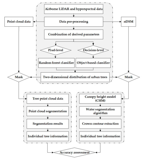
Figure 1.
Flowchart of Methodology.
3.2.1. Airborne LiDAR Dataset and Pre-Processing
The airborne LiDAR data with five returns were acquired on 22 June 2012 at a platform altitude of 609.6 m. The raw LiDAR point cloud data are shown in Figure 2.
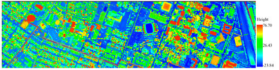
Figure 2.
The raw airborne light detection and ranging (LiDAR) point cloud data displayed in elevation mode. (unit: meter) (Data was provided by 2013 IEEE GRSS Data Fusion Contest).
Outlier Removal
Outlier removal is conducted in order to remove the point cloud noises and improve the data quality. Using a defined distance threshold, the neighboring points of each point are searched, and the average of the distances between each point and its neighboring points is calculated. The distance threshold is determined according to field situation, spatial resolution of the remote sensing data, several trial, and test. Then, the mean and standard deviation of all the average distances are calculated to determine the maximum distance using Equation (1). Finally, the average distance of a point to its neighbors is compared with the maximum distance. If the average distance of a point to its neighbors is much larger than the maximum distance, the point will be defined as an outlier and will be removed from the original point cloud data. Here, Dmaximum means the maximum distance, Dmean means the mean distance, Dstandard_deviation means standard derivation, and n is the number of neighboring points.
Dmaximum = Dmean + n*Dstandard_deviation
Extraction of Ground Points
The ground points were extracted based on an improved progressive triangulated irregular network (TIN) classification filtering algorithm [46]. Through seed points, a sparse TIN was generated. Then, layer-by-layer encryption was conducted iteratively until all ground points have been classified. The detailed steps are described as follows:
(1) Selection of initial seed point. As there are lots of buildings in this study area, the maximum building size (400 m) is taken as the grid size to grid the point cloud. Taking the lowest point in the grid as the starting seed point.
(2) Building a TIN. The initial seed point generated from the step: (1) was used to construct the initial triangulated irregular network (TIN).
(3) Iterative densification process. This process includes the following main steps: Traverse all the unclassified points, query the triangles that each point belongs to in the horizontal projection plane. Calculate the distance (d) from the point to the triangle and the maximum angle between the point and three vertices with the triangles plane. The distance and maximum angle are then compared with the iteration distance and iteration angle, separately. If it is less than the corresponding threshold, the point will be classified as a ground point and added to the triangulation. Repeat this process until all ground points have been classified.
Generation of Normalized Digital Surface Model (nDSM) and Intensity Imagery
The classified ground points were interpolated to produce a digital elevation model (DEM) using the inverse distance weight (IDW) interpolation method, whereas the first return points were interpolated with IDW interpolation method to produce a digital surface model (DSM). Finally, a normalized digital surface model (nDSM) was generated using Equation (2).
nDSM = DSM − DEM
The intensity attributes of the LiDAR point cloud data were also interpolated with IDW method. The spatial resolution of the generated raster data was set as 2.5 m × 2.5 m.
3.2.2. Hyperspectral Data and Pre-Processing
The hyperspectral image data was acquired on 23 June 2012 at a platform altitude of 1676.4 m, with 144 bands in the spectral range of 380–1050 nm. The spectral and spatial resolutions were 4.8 nm and 2.5 m, respectively. The airborne hyperspectral imagery was shown in Figure 3.
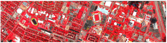
Figure 3.
The airborne hyperspectral data in false color display (data was provided by 2013 IEEE GRSS Data Fusion Contest).
In order to eliminate the influence of atmosphere, atmospheric correction was conducted on the original hyperspectral bands using the FLAASH model in ENVI 5.5 software. After atmospheric correction, in order to eliminate data redundancy, inverse minimum noise fraction rotation (MNF) and principal component analysis (PCA) were also conducted separately in ENVI 5.5 software [46,47,48,49,50,51]. Then, the first principal component was used to generate texture feature images based on the grey level co-occurrence matrix (GLCM). Finally, the normalized difference vegetation index (NDVI) was calculated using Equation (3). Here, represents the reflectance of NIR band (798 nm) and represents the reflectance of the far-red band (679 nm).
Finally, the first 22 bands of MNF (MNF22), nDSM, LiDAR intensity, NDVI, GLCM (GLCM mean, GLCM homogeneity, and GLCM dissimilarity) and the first two bands of PCA (PCA2) will be used in the following classification.
3.2.3. Training and Validation Samples
In this study, 12 classes were classified, including grass, grass_synthetic, trees, soil, water, building, road, highway, railway, parking_lot, tennis_court, and running_track. The training and validation samples for urban vegetation classification were all provided by the 2013 IEEE GRSS Data Fusion Contest [45], URL: http://www.grss-ieee.org/community/technical-commitees/data-fusion/. Detailed information on training and validation samples is shown in Table 1. Since the main goal of this study was to extract individual trees in complex urban areas, only the grasses and trees were listed in the following parts, and the rest 10 classes were defined as “others” in order to present the results clearly.

Table 1.
Details of training and validation samples used for urban vegetation extraction (Training and validation samples were all provided by 2013 IEEE GRSS Data Fusion Contest).
3.3. Spatial Extent Extraction of Urban Trees and Grasses Based on Hyperspectral and LIDAR Data
3.3.1. Extraction of Urban Trees and Grasses Using Random Forest Classification Method
Random Forest is a classification, prediction, and feature selection algorithm, which can process large amounts of data. In this paper, the random forest classification method was used to reduce dimension and classify the combined hyperspectral and LiDAR data (Figure 4). Firstly, the random forest-recursive feature elimination (RFE) method was used to analyze the importance of hyperspectral bands. According to the importance of the derived hyperspectral bands, the first 22 bands of MNF were selected to extract urban vegetation. Then the selected bands were combined with nDSM and intensity which were derived from LiDAR data. Finally, the combined bands of selected hyperspectral and LiDAR data were input into the random forest classification method to produce trees, grasses and 10 others classes (including building, water, railway, highway, parking_lot, tennis_court, running_track, soil, road, and grass_synthetic). The training samples and validation samples (Table 1) were all provided by the 2013 IEEE GRSS Data Fusion Contest [45], (URL: http://www.grssieee.org/community/technical-commitees/data-fusion/).
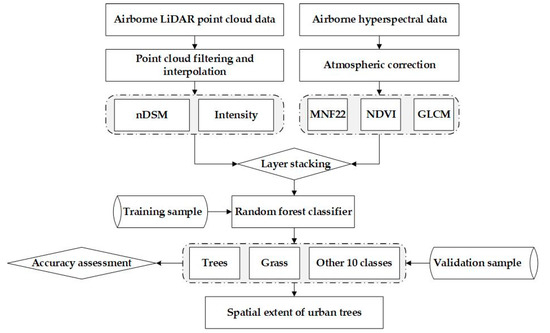
Figure 4.
Flowchart of random forest classification for urban vegetation extraction with hyperspectral and LiDAR data. Here other 10 classes include building, water, railway, highway, parking_lot, tennis_court, running_track, soil, road, and grass_synthetic.
Here, the MNF22+NDVI+GLCM+nDSM+Intensity bands combination was selected and input into the random forest classification method. The number of trees in the random forest was set to 1000.
3.3.2. Extraction of Urban Trees and Grasses Using Object-Based Classification Method
Object-based classification is based on objects not pixels, it cannot only make full use of spatial, texture, and spectral information of segmented objects, but also can avoid the “salt and pepper effect” of the random forest classification method. In addition, it can also define different bands with different weights, which could make full use of information from different bands. This section includes the following parts: image segmentation, object feature selection, classification, and accuracy assessment (Figure 5). In this paper, multi-resolution segmentation method in Definiens Developer 9.0 was used for image segmentation. The accuracy of image segmentation significantly influences the classification accuracy [52]. In order to get the optimal segmentation scale, the estimation of scale parameter 2 (ESP2) tool was used [53,54,55,56]. To extract grasses and trees, the rules were set as follows (Here trees whose height lower than 2 m were defined as shrubs):
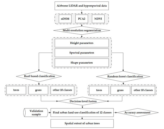
Figure 5.
Flowchart of object-based classification for urban trees and grasses extraction with hyperspectral and LiDAR data. Here other 10 classes include building, water, railway, highway, parking_lot, tennis_court, running_track, soil, road, and grass_synthetic.
- (1)
- Segment nDSM imagery with a scale of 2.
- (2)
- Mean nDSM ≥ 2 m and Mean NDVI ≥ 0.3.
- (3)
- Merge the extracted objects.
- (4)
- Assign the above class to tree.
- (5)
- Mean 0.5 < nDSM < 2 m and Mean NDVI ≥ 0.3.
- (6)
- Merge the extracted objects.
- (7)
- Assign the above class to shrub.
- (8)
- Mean 0 < nDSM < 0.5 m and Mean NDVI ≥ 0.3.
- (9)
- Assign the above class to grass.
However, there are too few shrubs in the study area, so the distribution of shrubs is ignored. As the classification accuracy of other 10 classes (including building, water, railway, highway, parking_lot, tennis_court, running_track, soil, road, and grass_synthetic) is relatively low using the rule object-based classification method, especially the classes with similar spectral information and without height information, including soil, road, highway, railway, and so on. Therefore, after multi-resolution segmentation on nDSM + PCA2 + NDVI combined parameters, random forest supervised classification method was also used to classify the segmented objects. The combined use of rule base and supervised random forest object-based classification method were much better than any single method, and the boundary of extracted trees was exported as a mask for the following process.
3.4. Individual Tree Segmentation Based on CHM Raster Data and Point Cloud Data
3.4.1. Segmentation of Individual Trees Based on CHM Raster Data
In urban areas, there are buildings, highways, and trees with different heights. Therefore, non-vegetation objects should be excluded to obtain the canopy height model (CHM). The two-dimensional boundaries of trees extracted by object-based classification method were used as a mask. Then, the nDSM raster was clipped by the tree mask to get the CHM raster data. As buildings were surrounded by trees, there were lots of small parts around the buildings which would increase the difficulty of CHM segmentation. Therefore, additional refinement was conducted on the gridded CHM raster data using morphological operators and majority filtering.
In order to identify and delineate individual trees, CHM segmentation was conducted by using the watershed segmentation method to isolate individual tree crowns [57]. Then, the information of individual trees was derived, such as tree location, crown diameter, tree height, and crown area. The flowchart of the CHM segmentation is shown in Figure 6.
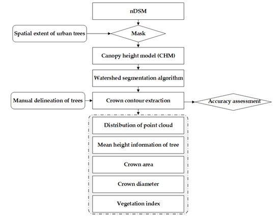
Figure 6.
Flowchart of individual tree segmentation based on canopy height model (CHM).
The gray value of CHM pixels represents the height of the objects. A catchment basin consists of a regional lowest point in the CHM and its affected areas, while a watershed is the boundary of the catchment basin. A watershed is delineated by simulating the immersion process. The resulting set of barriers can build a watershed by flooding, which is the segmentation result. The accuracy of CHM segmentation largely depends on the resolution of CHM and influenced by tree density and tree species.
3.4.2. Segmentation of Individual Trees Based on Point Cloud Data
Individual tree segmentation based on CHM could not represent the 3D crown morphology perfectly, because the canopy height model is based on the height difference of trees, and does not contain the information of the lower structure of the canopy. Different from CHM segmentation, point cloud segmentation can identify and segment individual trees directly using clustering point cloud data [58,59]. The advantage of this method is that it can preserve information under canopy.
The point cloud segmentation method developed by Li et al. [20] was used in this study. The premise of this method is to assume that there are always some gaps between trees. Firstly, seed points were selected by finding the local maximum points. Secondly, the individual trees were segmented based on the geometric relationship between the seed point and other points. The principle of this method is shown in Figure 7.
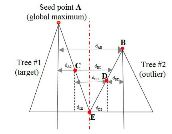
Figure 7.
The principle of point cloud segmentation algorithm.
As shown in the Figure 7, the seed point A is determined by the global maximum value, and the first tree is segmented. Then, a second tree is determined at the local maximum point B, and the horizontal distance between A and B is larger than the defined distance threshold. Following the minimum distance principle, every point is assigned to one of these two trees. For example, if the horizontal distance between C and A is smaller than the horizontal distance between C and B, then C will be assigned to the first segmented tree correspondingly. If the horizontal distance between E and A is the same as the horizontal distance between E and B, then E will be set as the boundary point between the two trees.
The defined distance threshold is important, as it can influence the accuracy of point cloud segmentation directly. If the defined distance threshold is too large or too small, the under-segmentation and over-segmentation will occur. In this study, the threshold is set as 1. The determination of the threshold is determined by trial and error. After segmentation, the structural metrics of each segmented trees were extracted directly from the three-dimensional LiDAR point cloud data, such as tree location, tree crown diameter, tree height, and crown area.
3.5. Accuracy Assessment
3.5.1. Accuracy Assessment of Classification Results
In this study, accuracy index and confusion matrix are used to conduct accuracy assessment of the classified urban vegetation maps [60,61]. Here, accuracy index (AI) is used to take commission and omission pixels into account for each land type [62,63]. The formula of AI is set as followed:
where n is the total number of correct samples, commission error (CE) is the number of commission samples and omission error (OE) is the number of omission samples. The kappa coefficient is also used and the equation of kappa is set as followed [64]:
where κ is the kappa coefficient; r is the number of rows; xi+ and x+i are the sums of all observations in row i and column i, xii is the observation in row i and column i (on the main diagonal), and N is the total number of samples [65]. Overall accuracy (OA) is the ratio of correctly classified numbers to total numbers of the validation samples. In this study, the same validation samples are used to assess overall accuracy in all classified maps.
3.5.2. Accuracy Assessment of Individual Tree Segmentation Results
Due to the precise visual interpretation, the digitized individual tree crown boundaries were considered as benchmark. The manually digitized method has been used in validation purpose for the extraction of individual trees in other studies [66,67]). Under normal conditionals, surveyed tree crown and tree location data would be used in the validation for individual tree extraction. However, due to the lack of surveyed data, Dai et al. (2018) delineated the crown boundaries and tree location manually from airborne laser scanning (ALS) point cloud data by visual interpretation for validation purposes [66]. Therefore, in this study, the visual interpretation of individual trees was conducted based on the 3D visualization of point cloud data, 3D visualization of CHM, and the hyperspectral data in false color. Firstly, the hyperspectral imagery in false color and the 2D extent boundaries of urban trees were overlaid, in order to digitize individual trees better. As for the trees difficult to classify, 3D visualization of tree point cloud data and CHM imagery was used to interpret trees visually. Then, the manually digitized individual trees were used as a reference layer. Finally, object-based accuracy assessment was conducted, as it is more meaningful than the raster output. There are two indicators including commission errors and omission errors, which were acquired by overlaying the CHM segmentation results and the reference layer [68]. With overlay analysis of reference data and the individual tree segmentation results, the raster product was extensively reviewed and edited though manual interpretation.
4. Results
4.1. Extraction Results of Urban Trees and Grasses Using Random Forest Classification Method and Object-Based Classification Method
In this paper, the main purpose was to extract urban grasses and individual trees from combined hyperspectral and LiDAR data. Therefore, although a total of 12 classes were classified (Figure 8), only the urban vegetation classes (trees and grasses) were listed in the following part. In addition, the performance of random forest classification method and object-based classification method for urban vegetation extraction were also explored by using combined hyperspectral and LiDAR data. The combined parameters for the random forest classification method were MNF22 + NDVI + intensity + nDSM + GLCM. The results indicated that the overall accuracy and kappa coefficient of random forest classification method was 95.87% and 0.9550, respectively. In order to compare the classification accuracy, the support vector machine (SVM) classification method was also used. The overall accuracy and kappa coefficient of SVM classification result were 95.11% and 0.9466, respectively. As for object-based classification method, the overall accuracy and kappa coefficient were 93.11% and 0.9286, respectively, which was not as good as the random forest classifier. However, the class-level accuracy of trees and grasses was as good as the random forest classifier. In addition, the results could also avoid the “salt and pepper effect”. The producer’s accuracy and user’s accuracy of trees and grasses are shown in the Table 2. The area of the extracted grasses was 711,481 m2. The distribution of extracted urban vegetation and all of the classes are shown in Figure 8.
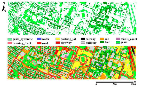
Figure 8.
Extracted urban vegetation (only include grasses and trees) with object-based classification method (top) and urban land use classification results (include all of the 12 classes) (bottom).
Table 2.
Error matrix of urban vegetation classification results with different classifiers based on hyperspectral and LiDAR data.
4.2. Results of Individual Tree Segmentation Based on CHM Raster Data and Point Cloud Data
Based on watershed segmentation method, the CHM was segmented to get the individual trees and tree groups. Information on the extracted trees, such as tree height, tree location, and crown area were also obtained. The canopy height model of the study area is showed in Figure 9. As the caption and legend suggest, Figure 9 is a canopy height model showing canopy heights in meters. Here, different heights of trees are shown in different colors. The boundaries of the individual trees extracted by CHM segmentation are also shown in Figure 10.
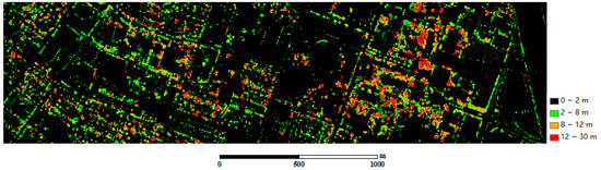
Figure 9.
Canopy height model (CHM) of the study area.
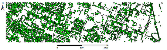
Figure 10.
Results of CHM segmentation (the black polygons are the boundaries of the segmented trees).
Due to the lack of field validation data about the tree height and crown diameter at the same period as remotely sensed image, a manual digitalizing method was used instead. A sample region that was appropriate for detecting the location and profile of the individual trees was selected. Then, the segmented tree crown areas based on the CHM segmentation were compared with the interpretation results. The number of extracted trees by CHM segmentation and manually delineated method were 4434 and 3828, with tree crown areas of 992,664 m2 and 986,086 m2, respectively. The root-mean-square error (RMSE) of tree locations was 1.8 m. The correctness of tree crown extraction was assessed only on a canopy-area basis by spatially overlaying the manually interpreted trees on the watershed segmented crowns. Compared with the manual results, CHM segmentation could segment individual trees correctly with a commission rate of 25% and an omission rate of 20%, and about 85% of the watershed segmented crowns were correctly segmented, except for small trees and large tree groups. The misclassified trees were very small individual trees with areas less than 5 m2 (tree crown diameter <2.5m), which is the spatial resolution of the used hyperspectral data and CHM raster. As for the big tree groups, it was difficult to detect individual trees correctly as the boundary of the trees were not obvious. The detailed information of the extracted trees is showed in Table 3.
Table 3.
Information on the extracted individual trees (10 samples).
Figure 11 shows the distribution of detected trees in manual interpretation (yellow polygons) and the CHM segmentation method (blue polygons), with most trees located within 2.5 m of the true location. In order to compare the CHM segmentation results clearly, the manual interpretation results (yellow polygons) and the segmentation results by the CHM segmentation method (blue) were overlaid on the CHM raster and hyperspectral imagery in false color, separately. From this figure, we can see small trees were missed. This was mainly because that the small trees (crown diameter less than 2.5 m) were only shown in one pixel which cannot be converted into a polygon. Figure 12 shows the enlarged view of the individual tree segmentation results in two- and three-dimensional aspect which can show the results more vividly. From Figure 12, we can conclude that the result of CHM segmentation has zigzag boundaries, which was mainly caused by the watershed segmentation algorithm, whereas the tree boundaries extracted by manual interpretation were much smoother. Figure 13 shows the vertical profiles of trees in different sizes including large individual trees, large tree groups, medium size individual trees, and small size individual trees. As can be seen in Figure 13, it is difficult to extract large tree groups and small-size individual trees.
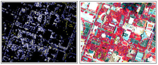
Figure 11.
CHM raster (left) and hyperspectral data (right) in false color composite with manual interpretation results (yellow polygons) and CHM segmentation results (blue polygons) for trees.
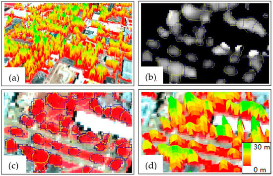
Figure 12.
(a) Three-dimensional display of urban trees; (b) enlarged view of segmentation results between manually interpreted trees (yellow polygons) and CHM segmentation results (blue polygons) with CHM as backdrop; (c) enlarged view of segmentation results between manually interpreted trees (yellow polygons) and CHM segmentation results (blue polygons) with hyperspectral imagery in false color as backdrop; and (d) three-dimensional display of (b,c).
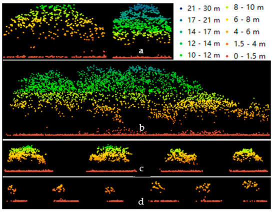
Figure 13.
LiDAR point cloud profiles of individual trees with different sizes: (a) large individual trees; (b) large tree groups; (c) medium size individual trees; and (d) small size individual trees.
Based on raw LiDAR point cloud data, individual trees were detected. The segmented individual trees are shown in Figure 14. In order to better observe the extracted individual trees, the enlarged view of the classification results is also shown in Figure 14b. In addition, the extracted individual trees based on point cloud data were also numbered by TreeID. Figure 15 and Figure 16 show the detailed point attribute information and three-dimensional view of the extracted individual trees. As the result of tree segmentation based on point cloud is difficult to evaluate quantitatively, manual delineation results and visual interpretation was conducted to compare the results of CHM and raw point cloud segmentation. Both methods could extract detailed information of individual trees, such as tree height, location, and crown diameter. The advantage of CHM segmentation is that its results could be compared with the CHM data and hyperspectral data directly. However, CHM is interpolated by raw point cloud data. There will be errors in the conversion of point cloud data to CHM raster data. Due to the influence of spatial resolution, there are also discontinuities around the crowns. Different from the results of CHM segmentation, individual tree segmentation based on point cloud data is much better as it can describe the trees in three dimensions especially the tree structure under canopy, whereas the CHM segmentation results are only for the top layer of tree canopies. In addition, the small trees can also be detected from point clouds, which is better than that of CHM segmentation.
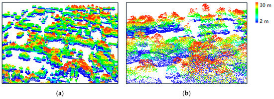
Figure 14.
(a) Results of individual tree segmentation based on point cloud data method displayed in three-dimensional visualization; (b) the enlarged view of individual tree segmentation results based on point cloud data method.
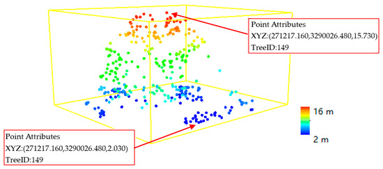
Figure 15.
Three-dimensional visualization of one typical individual tree extracted by point cloud data method. Here, points with different height were showed in different colors, and the attributes of selected points were showed in red boxes. The height of the tree crown from down to top is from 2.03 m to 15.73 m.
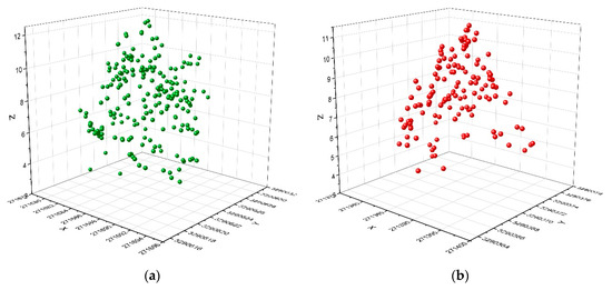
Figure 16.
Three-dimensional visualization of two typical individual trees extracted by point cloud data method. Here, X, Y is the location of the extracted trees, and Z is the height information of the extracted trees. Subfigure (a,b) mean three-dimensional visualization of two typical individual trees extracted by point cloud method, and (a) represents one tree and (b) represents
the other.
5. Discussion
5.1. Performance of Different Classification Methods for Trees and Grasses Extraction
With the rapid development of classification methods, many studies have been carried out with different classification methods. However, many challenges remain due to the complexity of urban environments. In this study, random forest classification method and object-based classification method were used to explore the advantages of combined hyperspectral and LiDAR data. The classification accuracy of these two methods were both over 99%, which could extract urban vegetation correctly. Although the classification accuracy of random forest and object-based classification method is almost the same, the advantages of these two methods are different. Object-based classification method is much better than the random forest classification method, mainly because it can reduce the salt and pepper effect.
The result of this paper can also be compared with other studies using combined hyperspectral and LiDAR data. Man et al. (2015) classified fifteen classes with hyperspectral and LiDAR data, and reported the producer’s accuracy (PA), user’s accuracy (UA), and accuracy index (AI) of the trees as 94.6%, 96.5%, and 91.5%, respectively [69]. Compared with the above results from the same study area, the producer’s accuracy (PA), user’s accuracy (UA), and accuracy index (AI) of the trees in this paper is 99.66%, 99.10%, and 99.99%, respectively, which is much higher. It can be concluded that the classification method can obtain excellent results for both random forest classifier and the object-based classifier. Man et al. (2019) extracted urban objects in shadow areas with hyperspectral and LiDAR data, and demonstrated the advantage of LiDAR data in improving the classification accuracy of urban objects in shadow areas, including trees and buildings [70]. The study has also shown that the combined use of airborne LiDAR and hyperspectral data could improve the classification accuracy of trees in shadow areas. Xia et al. (2018) used hyperspectral and LiDAR data to extract several types of grasses and trees. The classification accuracy of trees, grass_stressed, and grass_healthy is 91.76%, 88.63%, and 82.91%, respectively. Compared with the above results, the classification accuracy of grasses and trees is much higher. This was mainly because the hyperspectral data used in Xia et al. (2018) was highly affected by cloud shadows, and the classified grass types were also different. Therefore, due to the above different, it was difficult to compare the above results [34]. Li et al. (2013) used a hierarchical object-based classification method to classify urban vegetation with high-resolution aerial photography alone [71] and obtained a classification accuracy of 90.5%, which indicates that the object-based classification method was effective for vegetation mapping, including for trees and grasses. Xu et al. (2015) reviewed the application of fused airborne LiDAR and optical sensors in forest description [72]. The review demonstrated that the fusion of multiple remote sensing data could improve the performance of forest areas extraction (about 20% accuracy improvement). Alonzo et al. (2016) used hyperspectral imagery and LiDAR data for urban forest structure mapping and achieved accuracies of 93% and 83% for Pinus pinea and Quercus agrifolias, respectively [44]. Overall, the combined use of hyperspectral and LiDAR data resulted in high accuracy in urban vegetation extraction.
5.2. Performance of Individual Trees Detection Based on CHM Raster Data and Point Cloud Data
Because urban environments are complex, the measurement indicators of urban vegetation depend not only on the spatial distribution of urban vegetation, but also on the spatial structure of vegetation. Therefore, in this paper, CHM segmentation and point cloud segmentation were conducted to detect individual trees in two dimensions and three dimensions. As for CHM segmentation, the accuracy of CHM segmentation largely depends on the resolution of CHM and is influenced by tree density and tree species. CHM raster data is derived from LiDAR point cloud data, which will increase the number of errors during the conversion of point cloud data to CHM raster data, especially the tree crown boundary and the small trees (tree crown diameter <2.5 m). Take the small trees as an example, their crown diameter is less than 2.5 m which is the spatial resolution of the used hyperspectral data and CHM raster. Therefore, a small tree will be shown as one cell (2.5 m × 2.5 m) which will be very difficult to conduct CHM segmentation because watershed-based segmentation needs a group of connected pixels. In many cases, it is difficult to detect individual trees in large tree groups due to the lack of clear boundaries between individual tree crowns. As a result, the individual tree crown segmentations are not perfect because of overlapping branches from neighboring trees. In this study, about 85% of the watershed segmented crowns matched the results from visual interpretation, especially the medium-sized trees.
Different from CHM segmentation, point cloud segmentation can identify and segment most individual trees directly by clustering point cloud data, which can preserve the structure of the understory. In addition, the small trees (crown diameter <2.5 m) can also be segmented using the point cloud segmentation method, which is better than CHM segmentation methods. However, some large tree groups were misclassified as individual trees. So far, extracting single trees from large tree groups remains a challenge which may require improvements in both data and methodology. In complex urban environments, the machine learning classification methods and different segmentation methods have been used to extract individual trees in two- and three-dimensions. For example, MacFaden et al. (2012) used LiDAR data and object-based method to extract urban tree canopy in New York City with an overall accuracy of 96% [73]; Huang et al. (2013) estimated urban green volume with airborne LiDAR data and high-resolution remotely sensed images, and obtained a root-mean-square error (RMSE) of 1.66 m for segmented tree crowns [74]. Dai et al. (2018) proposed a new method for 3D individual tree extraction using multispectral LiDAR point clouds in Tobermory, Ontario, Canada, which might not be applicable to single wavelength laser scanning systems. However, due to the differences of different study areas, it is difficult to compare the results of this paper with other relevant studies.
6. Conclusions
This paper evaluated the performance of two classification methods in urban vegetation extraction, including the random forest classification method and the object-based classification method, and the performance of the two segmentation methods in individual tree extraction, including segmentation based on canopy height model (CHM) raster data and point cloud data. The following conclusions can be drawn from the results.
- (1)
- Because of the advantage of hyperspectral and LiDAR data combination, the classification accuracy of random forest classification method and object-based classification method were both over 99%. However, the object-based classification method is much better as it can avoid the salt and pepper effect, which is more suitable for urban trees extraction.
- (2)
- Compared with the manual results, about 85% of the watershed segmented crowns are correctly segmented, except for small trees and large tree groups. The missed small trees are mainly due to the spatial resolution of hyperspectral and CHM raster data. However, the segmentation based on raw LiDAR point cloud data can extract small individual trees more accurately, and can also reveal the understory. Individual tree segmentation from large tree groups is still a huge challenge, whether it is based on CHM segmentation or point cloud segmentation or manual digitization. In the future, improvement in both data and methodology could better solve this problem, such as the combined use of hyperspectral data and ground-based LiDAR data, and implementation of machine learning algorithms.
- (3)
- The two proposed methods for individual tree segmentation could provide detailed information of individual trees for urban forest managers, such as the location, height, and crown diameter. In addition, the results of individual tree extraction can also provide the basis for other studies, such as tree species classification, physiological state monitoring, and biomass estimation at individual tree level.
Author Contributions
Q.M. conceived and designed the methodology of the study, performed the data analysis and wrote the original draft; P.D. reviewed and edited the draft; and X.Y., Q.W., and R.H. reviewed the original draft and participated in discussion. All authors have read and agree to the published version of the manuscript.
Funding
This research is funded by Natural Science Foundation of Shandong Province (NO. ZR2016DB19) and Key Technology Research and Development Program of Shandong (2019GSF109034).
Acknowledgments
The first author would like to thank the Hyperspectral Image Analysis group and the NSF-Funded Center for Airborne Laser Mapping (NCALM) at the University of Houston for providing the data sets used in this study, and the IEEE GRSS Data Fusion Technical Committee for organizing the 2013 Data Fusion Contest.
Conflicts of Interest
The authors declare no conflict of interest. The funding sponsors had no role in the design of the study; in the collection, analyses, or interpretation of data; in the writing of the manuscript, and in the decision to publish the results.
References
- Sun, C.; Wu, Z.; Lv, Z.; Yao, N.; Wei, J. Quantifying different types of urban growth and the change dynamic in Guangzhou using multi-temporal remote sensing data. Int. J. Appl. Earth Obs. Geoinf. 2013, 21, 409–417. [Google Scholar] [CrossRef]
- Armson, D.; Stringer, P.; Ennos, A.R. The effect of tree shade and grass on surface and globe temperatures in an urban area. Urban For. Urban Green. 2012, 11, 245–255. [Google Scholar] [CrossRef]
- Akbari, H. Shade trees reduce building energy use and CO2 emissions from power plants. Environ. Pollut. 2002, 116, S119–S126. [Google Scholar] [CrossRef]
- Fang, C.F.; Ling, D.L. Investigation of the noise reduction provided by tree belts. Landsc. Urban plan. 2003, 63, 187–195. [Google Scholar] [CrossRef]
- Myint, S.W.; Brazel, A.; Okin, G.; Buyantuyev, A. Combined effects of impervious surface and vegetation cover on air temperature variations in a rapidly expanding desert city. Gisci. Remote Sens. 2010, 47, 301–320. [Google Scholar] [CrossRef]
- Tyrväinen, L.; Mäkinen, K.; Schipperijn, J. Tools for mapping social values of urban woodlands and other green areas. Landsc. Urban plan. 2007, 79, 5–19. [Google Scholar] [CrossRef]
- Peña-Barragán, J.M.; Ngugi, M.K.; Plant, R.E.; Six, J. Object-based crop identification using multiple vegetation indices, textural features and crop phenology. Remote Sens. Environ. 2011, 115, 1301–1316. [Google Scholar] [CrossRef]
- Slaev, A.D. The relationship between planning and the market from the perspective of property rights theory: A transaction cost analysis. Plan. Theory 2017, 16, 404–424. [Google Scholar] [CrossRef]
- Van der Krabben, E. A Property Rights Approach to Externality Problems: Planning Based on Compensation Rules. Urban Stud. 2009, 46, 2869–2890. [Google Scholar] [CrossRef]
- Shahab, S.; Viallon, F.X. Swiss Land Improvement Syndicates: ‘Impure’ Coasian Solutions. Plan. Theory 2020. [Google Scholar] [CrossRef]
- Shahab, S.; Viallon, F.X. A Transaction-cost Analysis of Swiss Land Improvement Syndicates. Town Plan. Rev. 2019, 90, 545–565. [Google Scholar] [CrossRef]
- Herold, M.; Roberts, D.A.; Gardner, M.E.; Dennison, P.E. Spectrometry for urban area remote sensing—Development and analysis of a spectral library from 350 to 2400 nm. Remote Sens. Environ. 2004, 91, 304–319. [Google Scholar] [CrossRef]
- Awrangjeb, M.; Ravanbakhsh, M.; Fraser, C.S. Automatic detection of residential buildings using LIDAR data and multispectral imagery. ISPRS J. Photogramm. 2010, 65, 457–467. [Google Scholar] [CrossRef]
- Rottensteiner, F. Automatic Generation of High-Quality Building Models from Lidar Data. IEEE Comput. Graph. 2003, 23, 42–50. [Google Scholar] [CrossRef]
- Jensen, J.; Cowen, D. Remote sensing of urban suburban infrastructure and socio-economic attributes. Photogramm. Eng. Remote Sens. 1999, 65, 611–622. [Google Scholar]
- Clark, M.L.; Roberts, D.A.; Clark, D.B. Hyperspectral discrimination of tropical rain forest tree species at leaf to crown scales. Remote Sens. Environ. 2005, 96, 375–398. [Google Scholar] [CrossRef]
- Dalponte, M.; Bruzzone, L.; Gianelle, D. Tree species classification in the Southern Alps based on the fusion of very high geometrical resolution multispectral/hyperspectral images and LiDAR data. Remote Sens. Environ. 2012, 123, 258–270. [Google Scholar] [CrossRef]
- Alonzo, M.; Bookhagen, B.; Roberts, D.A. Urban tree species mapping using hyperspectral and LiDAR data fusion. Remote Sens. Environ. 2014, 148, 70–83. [Google Scholar] [CrossRef]
- Kwak, D.A.; Lee, W.K.; Lee, J.H.; Biging, G.S.; Gong, P. Detection of individual trees and estimation of tree height using LiDAR data. J. For. Res. Jpn. 2007, 12, 425–434. [Google Scholar] [CrossRef]
- Li, W.; Guo, Q.; Jakubowski, M.K.; Kelly, M. A New Method for Segmenting Individual Trees from the Lidar Point Cloud. Photogramm. Eng. Remote Sens. 2012, 78, 75–84. [Google Scholar] [CrossRef]
- Youngentob, K.N.; Roberts, D.A.; Held, A.A.; Dennison, P.E.; Jia, X.; Lindenmayer, D.B. Mapping two Eucalyptus subgenera using multiple endmember spectral mixture analysis and continuum-removed imaging spectrometry data. Remote Sens. Environ. 2011, 115, 1115–1128. [Google Scholar] [CrossRef]
- Powell, R.L.; Roberts, D.A.; Dennison, P.E.; Hess, L.L. Sub-pixel mapping of urban land cover using multiple endmember spectral mixture analysis: Manaus, Brazil. Remote Sens. Environ. 2007, 106, 253–267. [Google Scholar] [CrossRef]
- Liu, X.; Bo, Y. Object-based crop species classification based on the combination of airborne hyperspectral images and LiDAR data. Remote Sens. 2015, 7, 922–950. [Google Scholar] [CrossRef]
- Liu, W.; Yamazaki, F. Object-based shadow extraction and correction of high-resolution optical satellite images. IEEE J. STARS 2012, 5, 1296–1302. [Google Scholar] [CrossRef]
- Guan, H.; Li, J.; Chapman, M.; Deng, F.; Ji, Z.; Yang, X. Integration of orthoimagery and lidar data for object-based urban thematic mapping using random forests. Int. J. Remote Sens. 2013, 34, 5166–5186. [Google Scholar] [CrossRef]
- Qiong, W.; Ruofei, Z.; Wenji, Z.; Kai, S.; Liming, D. Land-cover classification using GF-2 images and airborne lidar data based on Random Forest. Int. J. Remote Sens. 2018, 40, 2410–2426. [Google Scholar]
- Rasti, B.; Ghamisi, P.; Plaza, J.; Plaza, A. Fusion of Hyperspectral and LiDAR Data Using Sparse and Low-Rank Component Analysis. IEEE Trans. Geosci. Remote Sens. 2017, 55, 6354–6365. [Google Scholar] [CrossRef]
- Wang, H.; Glennie, C. Fusion of waveform LiDAR data and hyperspectral imagery for land cover classification. ISPRS J. Photogramm. Remote Sens. 2015, 108, 1–11. [Google Scholar] [CrossRef]
- Luo, S.; Wang, C.; Xi, X.; Zeng, H.; Li, D.; Xia, S.; Wang, P. Fusion of Airborne Discrete-Return LiDAR and Hyperspectral Data for Land Cover Classification. Remote Sens. 2016, 8, 3. [Google Scholar] [CrossRef]
- Zhong, Y.; Cao, Q.; Zhao, J. Optimal Decision Fusion for Urban Land-Use/Land-Cover Classification Based on Adaptive Differential Evolution Using Hyperspectral and LiDAR Data. Remote Sens. 2017, 9, 868. [Google Scholar] [CrossRef]
- Chen, Y.; Li, C.; Ghamisi, P.; Jia, X.; Gu, Y. Deep Fusion of Remote Sensing Data for Accurate Classification. IEEE Geosci. Remote Sens. Lett. 2017, 14, 1253–1257. [Google Scholar] [CrossRef]
- Xu, X.; Li, W.; Ran, Q.; Du, Q.; Gao, L.; Zhang, B. Multisource Remote Sensing Data Classification Based on Convolutional Neural Network. IEEE Trans. Geosci. Remote Sens. 2018, 56, 937–949. [Google Scholar] [CrossRef]
- Forzieri, G.; Tanteri, L.; Moser, G.; Catani, F. Mapping natural and urban environments using airborne multi-sensor ADS40-MIVIS-LiDAR synergies. Int. J. Appl. Earth Obs. Geoinf. 2013, 23, 313–323. [Google Scholar] [CrossRef]
- Xia, J.; Yokoya, N.; Iwasaki, A. Fusion of hyperspectral and LiDAR data with a novel ensemble classifier. IEEE Geosci. Remote Sens. Lett. 2018, 15, 957–961. [Google Scholar] [CrossRef]
- Vosselman, G.; Kessels, P.; Gorte, B. The utilization of airborne laser scanning for mapping. Int. J. Appl. Earth Obs. Geoinf. 2005, 6, 177–186. [Google Scholar] [CrossRef]
- Yu, B.; Liu, H.; Zhang, L.; Wu, J. An object-based two-stage method for a detailed classification of urban landscape components by integrating airborne LiDAR and color infrared image data: A case study of downtown Houston. In Proceedings of the 2009 Joint Urban Remote Sensing Event, Shanghai, China, 20–22 May 2009. [Google Scholar]
- Chadwick, J. Integrated LiDAR and IKONOS multi-spectral imagery for mapping mangrove distribution and physical properties. Int. J. Remote Sens. 2011, 32, 6765–6781. [Google Scholar] [CrossRef]
- Delm, A.V.; Gulinck, H. Classification and quantification of green in the expanding urban and semi-urban complex: Application of detailed field data and IKONOS-imagery. Ecol. Indic. 2011, 11, 52–60. [Google Scholar] [CrossRef]
- Asner, G.P.; Knapp, D.E.; Kennedy-Bowdoin, T.; Jones, M.O.; Martin, R.E.; Boardman, J. Invasive species detection in Hawaiian rainforests using airborne imaging spectroscopy and LiDAR. Remote Sens. Environ. 2008, 112, 1942–1955. [Google Scholar] [CrossRef]
- Lucas, R.M.; Lee, A.C.; Bunting, P.J. Retrieving forest biomass through integration of CASI and LiDAR data. Int. J. Remote Sens. 2008, 29, 1553–1577. [Google Scholar] [CrossRef]
- Liu, L.; Nicholas, C.C.; Aven, N.W.; Pang, Y. Mapping urban tree species using integrated airborne hyperspectral and LiDAR remote sensing data. Remote Sens. Environ. 2017, 200, 170–182. [Google Scholar] [CrossRef]
- Man, Q.; Dong, P.; Guo, H.; Liu, G.; Shi, R. Light detection and ranging and hyperspectral data for estimation of forest biomass: A review. J. Appl. Remote Sens. 2014, 8, 69–72. [Google Scholar] [CrossRef]
- Gu, Y.; Wang, Q.; Jia, X.; Benediktsson, J.A. A Novel MKL Model of Integrating LiDAR Data and MSI for Urban Area Classification. IEEE Trans. Geosci. Remote Sens. 2015, 53, 5312–5326. [Google Scholar]
- Alonzo, M.; Mcfadden, J.P.; Nowak, D.J.; Roberts, D.A. Mapping urban forest structure and function using hyperspectral imagery and LiDAR data. Urban For. Urban Gree. 2016, 17, 135–147. [Google Scholar] [CrossRef]
- Debes, C.; Merentitis, A.; Heremans, R.; Hahn, J.; Frangiadakis, N.; Van Kasteren, T.; Liao, W.; Bellens, R.; Pizurica, A.; Gautama, S.; et al. Hyperspectral and LiDAR Data Fusion: Outcome of the 2013 GRSS Data Fusion Contest. IEEE J. STARS 2014, 7, 2405–2418. [Google Scholar] [CrossRef]
- Zhao, X.; Guo, Q.; Su, Y.; Xue, B. Improved progressive TIN densification filtering algorithm for airborne LiDAR data in forested areas. Isprs J. Photogramm. Remote Sens. 2016, 117, 79–91. [Google Scholar] [CrossRef]
- Lee, J.B.; Woodyatt, A.S.; Berman, M. Enhancement of High Spectral Resolution Remote Sensing Data by a Noise-Adjusted Principal Components Transform. IEEE Trans. Geosci. Remote Sens. 1990, 28, 295–304. [Google Scholar] [CrossRef]
- Galvão, L.S.; Formaggio, A.R.; Tisot, D.A. Discrimination of Sugarcane Varieties in Southeastern Brazil with EO-1 Hyperion Data. Remote Sens. Environ. 2005, 94, 523–534. [Google Scholar] [CrossRef]
- Pengra, B.W.; Johnston, C.A.; Loveland, T.R. Mapping an Invasive Plant, Phragmites Australis, in Coastal Wetlands Using the EO-1 Hyperion Hyperspectral Sensor. Remote Sens. Environ. 2007, 108, 74–81. [Google Scholar] [CrossRef]
- Binal, C.; Krishnayya, N.S.R. Classification of Tropical Trees Growing in a Sanctuary Using Hyperion (EO-1) and SAM Algorithm. Curr. Sci. 2009, 96, 1601–1607. [Google Scholar]
- Pignatti, S.; Cavalli, R.M.; Cuomo, V.; Fusilli, L.S.; Pascucci, S.; Poscolieri, M. Evaluating Hyperion Capability for Land Cover Mapping in a Fragmented Ecosystem: Pollino National Park, Italy. Remote Sens. Environ. 2009, 113, 622–634. [Google Scholar] [CrossRef]
- Kiani, K.; Mojaradi, B.; Esmaeily, A.; Salehi, B. Urban Area Object-based Classification by Fusion of Hyperspectral and LiDAR Data. In Proceedings of the 2014 IEEE Geoscience and Remote Sensing Symposium, Quebec City, QC, Canada, 13–18 July 2014; pp. 4832–4835. [Google Scholar]
- Drăgut, L.; Tiede, D.; Levick, S.R. ESP: A Tool to Estimate Scale Parameter for Multiresolution Image Segmentation of Remotely Sensed Data. Int. J. Geogr. Inf. Sci. 2010, 24, 859–871. [Google Scholar] [CrossRef]
- Belgiu, M.; Csillik, O. Sentinel-2 Cropland Mapping Using Pixel-based and Object-based Time-Weighted Dynamic TimeWarping Analysis. Remote Sens. Environ. 2017, 204, 509–523. [Google Scholar] [CrossRef]
- Drăgut, L.; Csillik, O.; Eisank, C.; Tiede, D. Automated Parameterisation for Multi-scale Image Segmentation on Multiple Layers. ISPRS J. Photogramm. Remote Sens. 2014, 88, 119–127. [Google Scholar] [CrossRef] [PubMed]
- Novelli, A.; Aguilar, M.; Aguilar, F.; Nemmaoui, A.; Tarantino, E. AssesSeg-A Command Line Tool to Quantify Image Segmentation Quality: A Test Carried Out in Southern Spain from Satellite Imagery. Remote Sens. 2017, 9, 40. [Google Scholar] [CrossRef]
- Chen, Q.; Baldocchi, D.; Gong, P.; Kelly, M. Isolating Individual Trees in a Savanna Woodland Using Small Footprint Lidar Data. Photogramm. Eng. Rem. Remote Sens. 2006, 72, 923–932. [Google Scholar] [CrossRef]
- Ferraz, A.; Bretar, F.; Jacquemoud, S.; Gonçalves, G.; Pereira, L.; Tomé, M. 3-D mapping of a multi-layered Mediterranean forest using ALS data. Remote Sens. Environ. 2012, 121, 210–223. [Google Scholar] [CrossRef]
- Reitberger, J.; Schnörr, C.; Krzystek, P.; Stilla, U. 3D segmentation of single trees exploiting full waveform LIDAR data. ISPRS J. Photogramm. Remote Sens. 2009, 64, 561–574. [Google Scholar] [CrossRef]
- Congalton, R.G. A Review of Assessing the Accuracy of Classifications of Remotely Sensed Data. Remote Sens. Environ. 1991, 37, 35–46. [Google Scholar] [CrossRef]
- Stehman, S.V. Selecting and Interpreting Measures of Thematic Classification Accuracy. Remote Sens. Environ. 1997, 62, 77–89. [Google Scholar] [CrossRef]
- Antonarakis, A.S.; Richards, K.S.; Brasington, J. Object-Based Land Cover Classification Using Airborne Lidar. Remote Sens. Environ. 2008, 112, 2988–2998. [Google Scholar] [CrossRef]
- Pouliot, D.A.; King, D.J.; Bell, F.W.; Pitt, D.G. Automated Tree Crown Detection and Delineation in High-Resolution Digital Camera Imagery of Coniferous Forest Regeneration. Remote Sens. Environ. 2002, 82, 322–334. [Google Scholar] [CrossRef]
- Foody, G.M. Status of Land Cover Classification Accuracy Assessment. Remote Sens. Environ. 2002, 80, 185–201. [Google Scholar] [CrossRef]
- Koetz, B.; Morsdorf, F.; Van Der Linden, S.; Curt, T.; Allgöwer, B. Multi-Source Land Cover Classification for Forest Fire Management Based on Imaging Spectrometry and Lidar Data. For. Ecol. Manag. 2008, 256, 263–271. [Google Scholar] [CrossRef]
- Dai, W.; Yang, B.; Dong, Z.; Shaker, A. A new method for 3D individual tree extraction using multispectral airborne LiDAR point clouds. ISPRS J. Photogramm. Remote Sens. 2018, 144, 400–411. [Google Scholar] [CrossRef]
- Strîmbu, V.F.; Strîmbu, B.M. A graph-based segmentation algorithm for tree crown extraction using airborne LiDAR data. ISPRS J. Photogramm. Remote Sens. 2015, 104, 30–43. [Google Scholar] [CrossRef]
- Ragia, L.; Winter, S. Contributions to a quality description of areal objects in spatial data sets. ISPRS J. Photogramm. Remote Sens. 2000, 55, 201–213. [Google Scholar] [CrossRef]
- Man, Q.; Dong, P.; Guo, H. Pixel-and feature-level fusion of hyperspectral and lidar data for urban land-use classification. Int. J. Remote Sens. 2015, 36, 1618–1644. [Google Scholar] [CrossRef]
- Man, Q.; Dong, P. Extraction of Urban Objects in Cloud Shadows on the basis of Fusion of Airborne LiDAR and Hyperspectral Data. Remote Sens. 2019, 11, 713. [Google Scholar] [CrossRef]
- Li, X.; Shao, G. Object-based urban vegetation mapping with high-resolution aerial photography as a single data source. Int. J. Remote Sens. 2013, 34, 19. [Google Scholar] [CrossRef]
- Xu, C.; Morgenroth, J.; Manley, B. Integrating Data from Discrete Return Airborne LiDAR and Optical Sensors to Enhance the Accuracy of Forest Description: A Review. Curr. For. Rep. 2015, 1, 206–219. [Google Scholar] [CrossRef]
- Macfaden, S.W.; O’Neil-Dunne, J.P.; Royar, A.R.; Lu, J.W.T.; Rundle, A.G. High-resolution tree canopy mapping for New York City using LIDAR and object-based image analysis. J. Appl. Remote Sens. 2012, 6, 3567. [Google Scholar] [CrossRef]
- Huang, Y.; Bailang, Y.; Zhou, J.; Hu, C.; Tan, W.; Hu, Z.; Wu, J. Toward automatic estimation of urban green volume using airborne LiDAR data and high-resolution Remote Sensing images. Front. Earth Sci. 2013, 7, 43–54. [Google Scholar] [CrossRef]
© 2020 by the authors. Licensee MDPI, Basel, Switzerland. This article is an open access article distributed under the terms and conditions of the Creative Commons Attribution (CC BY) license (http://creativecommons.org/licenses/by/4.0/).