High Ethylene and Propylene in an Area Dominated by Oil Production


Abstract
1. Introduction
2. Methods
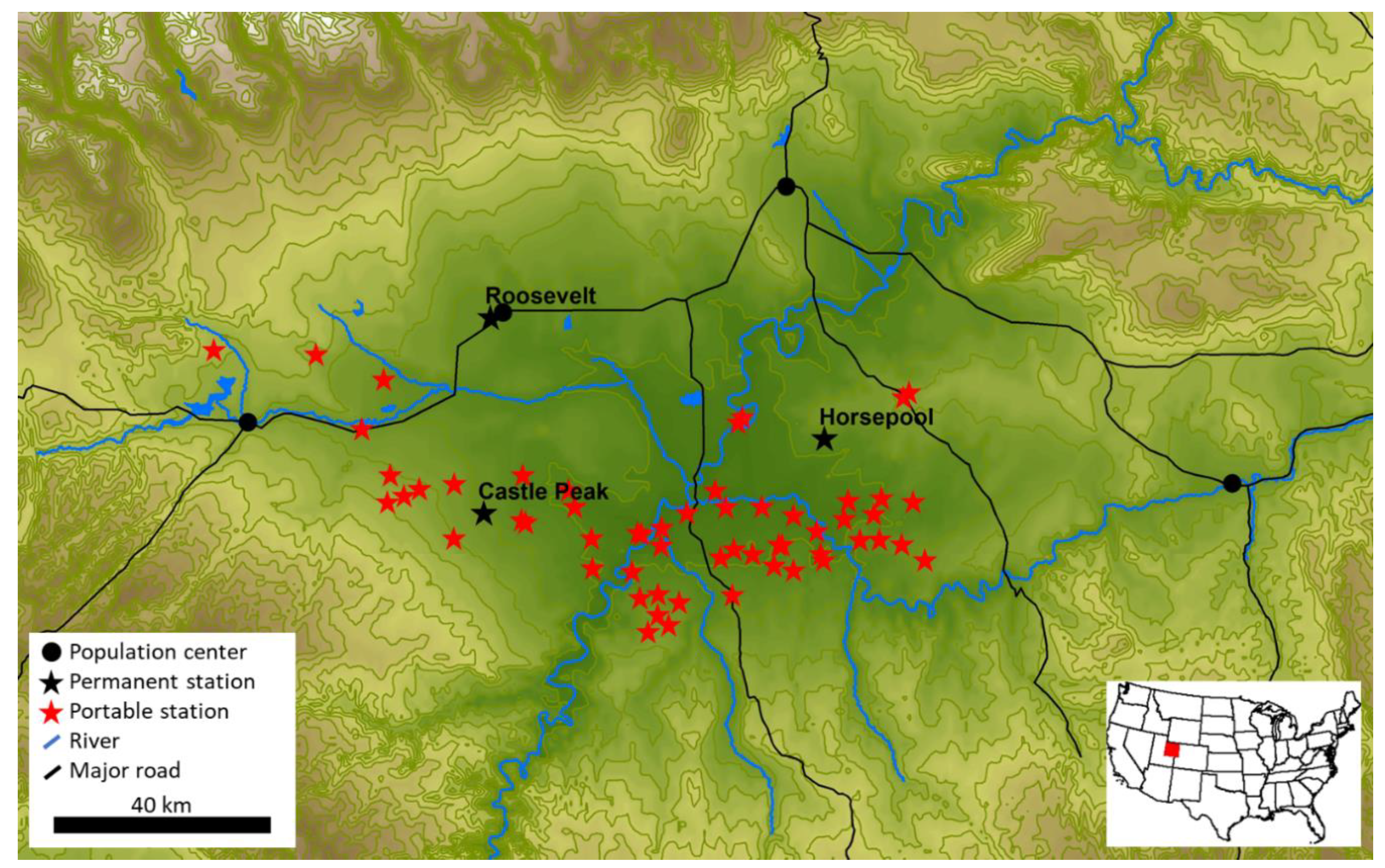
2.1. Study Location
2.2. Portable Sampling Stations
2.3. Permanent Monitoring Stations
2.4. Laboratory Analysis
2.5. Oil and Gas Industry Data
2.6. Statistical Analysis
- (a)
- Average elevation
- (b)
- Number of engines
- (c)
- Total engine organic compound emissions
- (d)
- Number of gas-fueled engines
- (e)
- Number of artificial lift engines
- (f)
- Number of two-stroke engines
- (g)
- Number of produced water ponds
- (h)
- Total area of produced water ponds
- (i)
- Number of glycol dehydrators
- (j)
- Total dehydrator organic compound emissions
- (k)
- Number of liquid storage tanks
- (l)
- Number of controls on liquid storage tanks
- (m)
- Number of producing oil and gas wells
- (n)
- Total amount of oil, gas, and water production
2.7. Quality Assurance
3. Results and Discussion
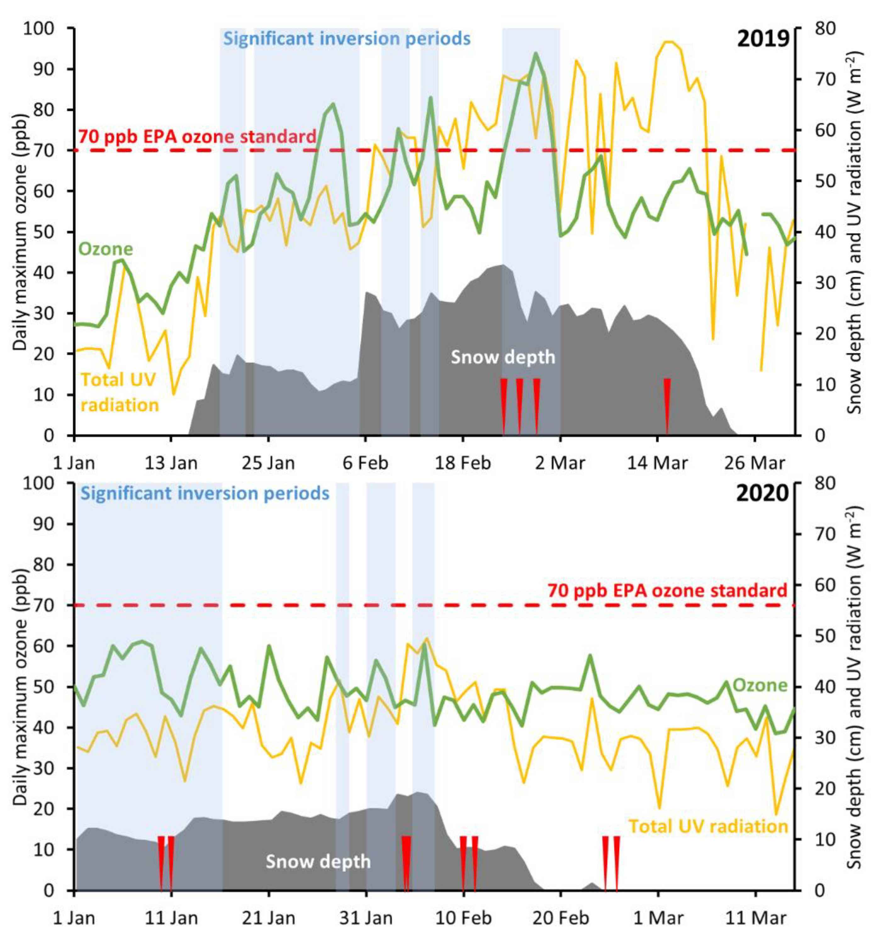
3.1. Impact of Inversion Conditions on Organic Compound Concentrations
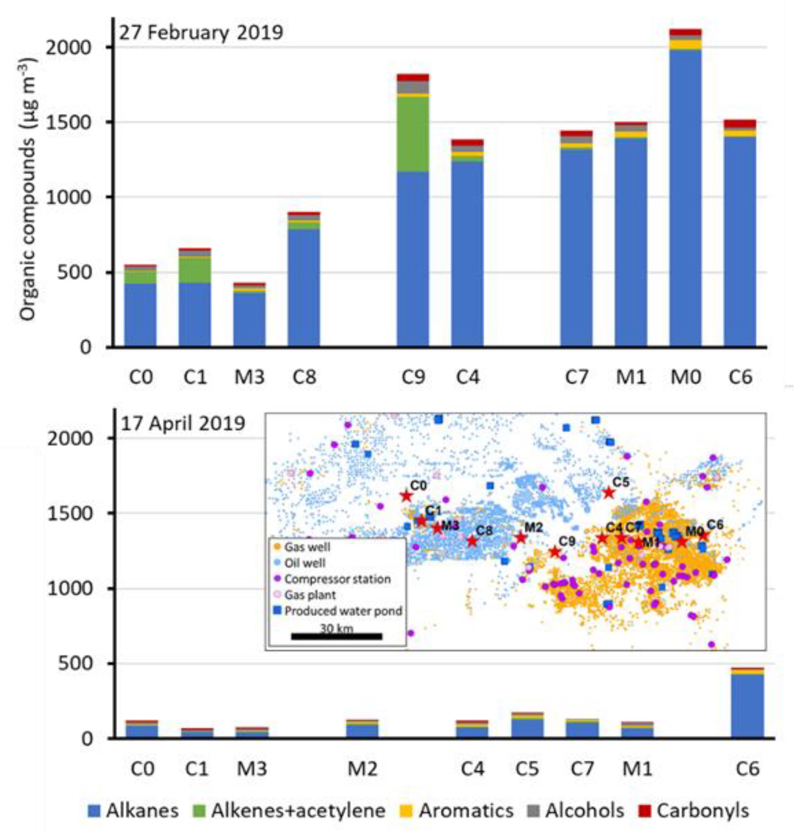
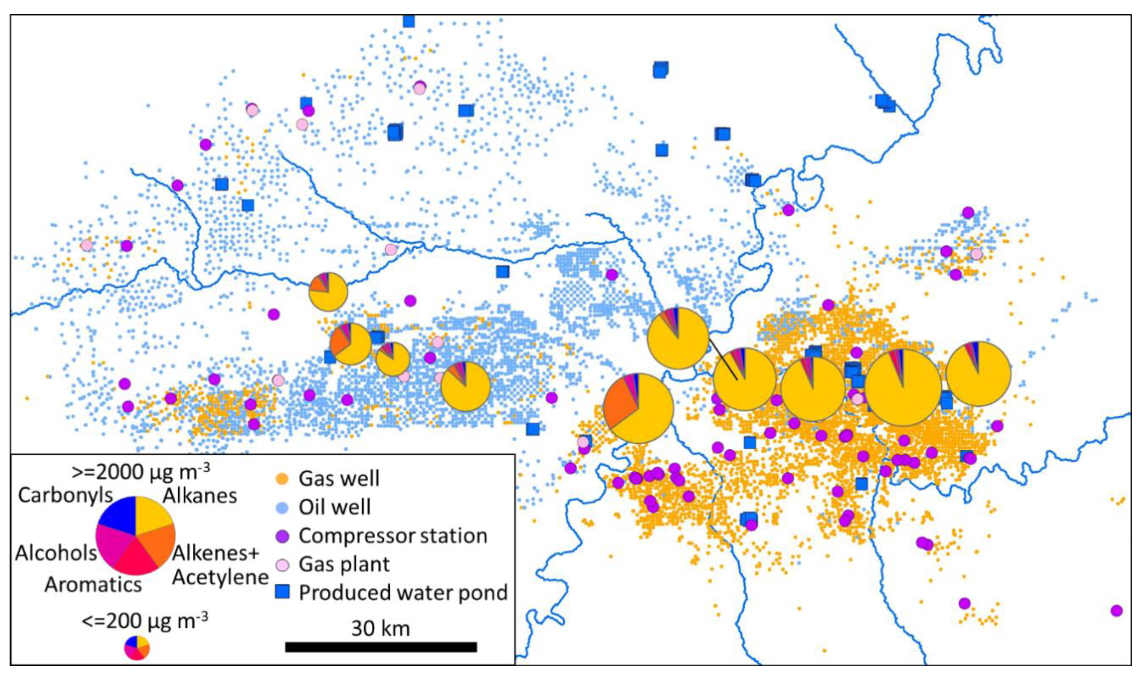
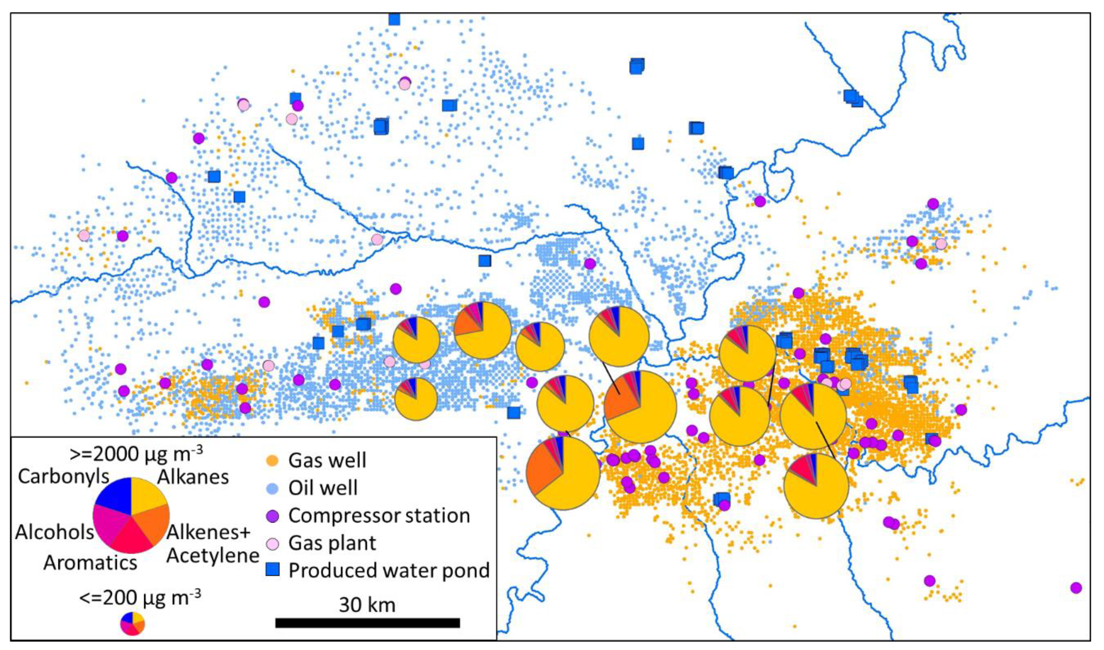
3.2. Spatial Distribution
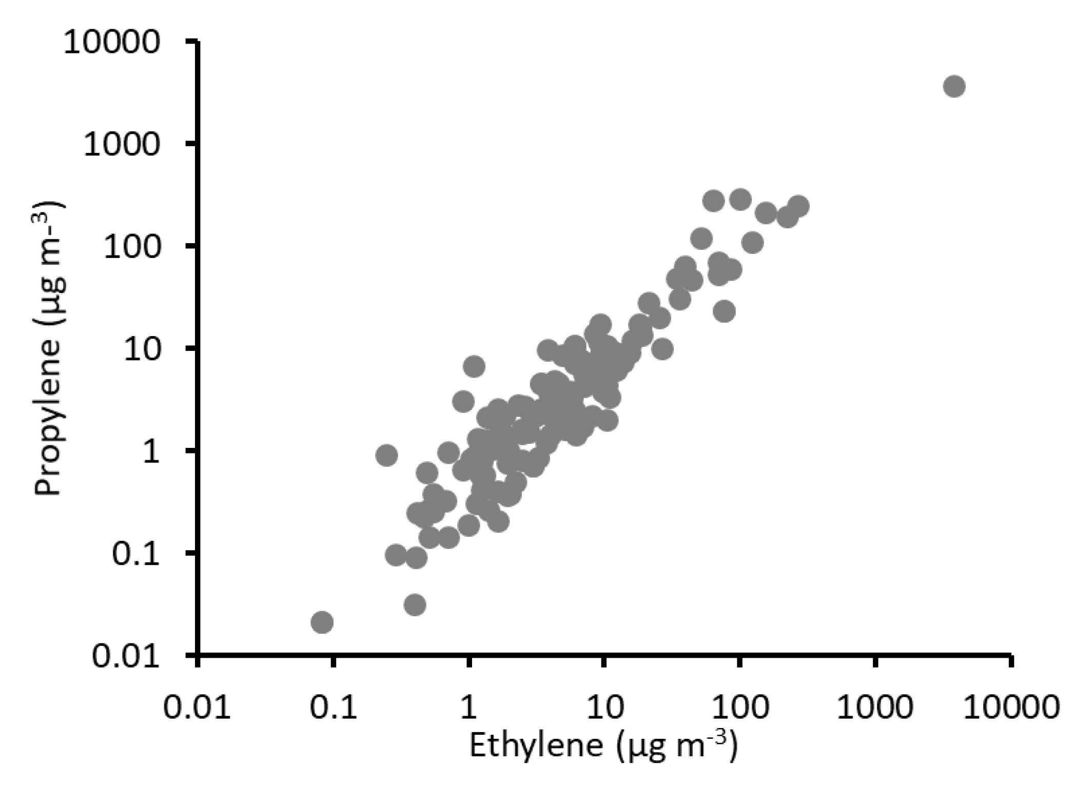
3.3. Sources of Alkenes in Oil-Producing Areas
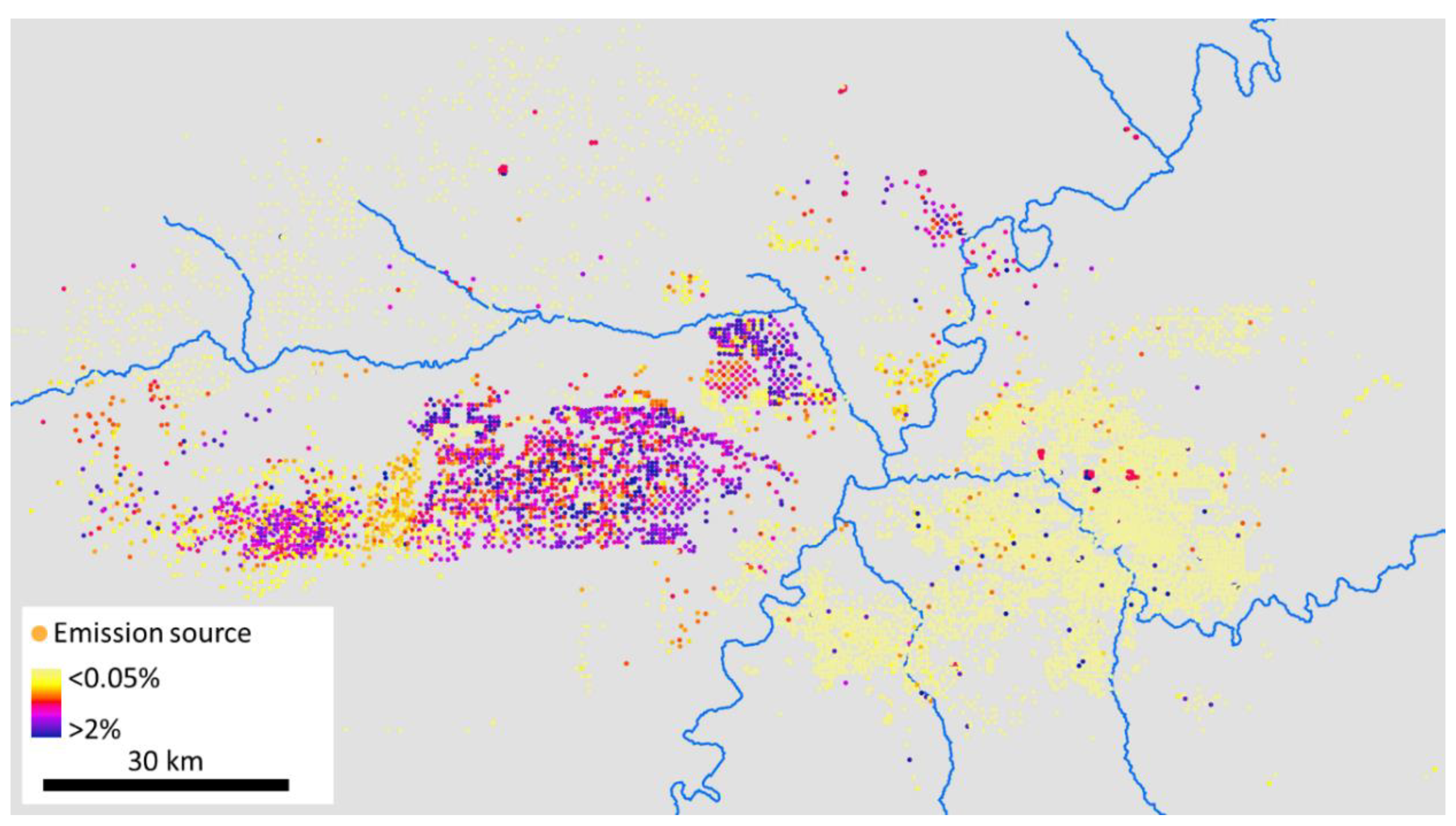
3.4. Comparison with Inventoried Emissions
4. Conclusions
Supplementary Materials
Author Contributions
Funding
Data Availability Statement
Conflicts of Interest
References
- Ahmadov, R.; McKeen, S.; Trainer, M.; Banta, R.; Brewer, A.; Brown, S.; Edwards, P.M.; De Gouw, J.; Frost, G.J.; Gilman, J.; et al. Understanding high wintertime ozone pollution events in an oil- and natural gas-producing region of the western US. Atmos. Chem. Phys. Discuss. 2015, 15, 411–429. [Google Scholar] [CrossRef]
- Edwards, P.M.; Brown, S.S.; Roberts, J.M.; Ahmadov, R.; Banta, R.M.; Degouw, J.A.; Dubé, W.P.; Field, R.A.; Flynn, J.H.; Gilman, J.B.; et al. High winter ozone pollution from carbonyl photolysis in an oil and gas basin. Nature 2014, 514, 351–354. [Google Scholar] [CrossRef]
- Matichuk, R.; Tonnesen, G.; Luecken, D.; Gilliam, R.; Napelenok, S.L.; Baker, K.R.; Schwede, D.; Murphy, B.; Helmig, D.; Lyman, S.N.; et al. Evaluation of the Community Multiscale Air Quality Model for Simulating Winter Ozone Formation in the Uinta Basin. J. Geophys. Res. Atmos. 2017, 122, 13545–13572. [Google Scholar] [CrossRef]
- Schnell, R.; Johnson, B.J.; Oltmans, S.J.; Cullis, P.; Sterling, C.; Hall, E.; Jordan, A.F.; Helmig, D.; Pétron, G.; Ahmadov, R.; et al. Quantifying wintertime boundary layer ozone production from frequent profile measurements in the Uinta Basin, UT, oil and gas region. J. Geophys. Res. Atmos. 2016, 121. [Google Scholar] [CrossRef]
- Mansfield, M.L.; Hall, C.F. A survey of valleys and basins of the western United States for the capacity to produce winter ozone. J. Air Waste Manag. Assoc. 2018, 68, 909–919. [Google Scholar] [CrossRef]
- Oltmans, S.J.; Schnell, R.C.; Johnson, B.; Pétron, G.; Mefford, T.; Neely, R. Anatomy of wintertime ozone associated with oil and natural gas extraction activity in Wyoming and Utah. Lementa Sci. Anthr. 2014, 2, 000024. [Google Scholar] [CrossRef]
- Lyman, S.N.; Tran, T. Inversion structure and winter ozone distribution in the Uintah Basin, Utah, U.S.A. Atmos. Environ. 2015, 123, 156–165. [Google Scholar] [CrossRef]
- Foster, C.S.; Crosman, E.T.; Holland, L.; Mallia, D.V.; Fasoli, B.; Bares, R.; Horel, J.; Lin, J.C. Confirmation of Elevated Methane Emissions in Utah’s Uintah Basin with Ground-Based Observations and a High-Resolution Transport Model. J. Geophys. Res. Atmos. 2017, 122, 13026–13044. [Google Scholar] [CrossRef]
- Foster, C.S.; Crosman, E.T.; Horel, J.D.; Lyman, S.N.; Fasoli, B.; Bares, R.; Lin, J.C. Quantifying methane emissions in the Uintah Basin during wintertime stagnation episodes. Elem. Sci. Anthr. 2019, 7, 24. [Google Scholar] [CrossRef]
- UDAQ. Uinta Basin: 2014 Air Agencies Oil and Gas Emissions Inventory. Available online: https://deq.utah.gov/legacy/destinations/u/uintah-basin/air-agencies-emissions-inventory/index.htm (accessed on 1 July 2020).
- Lyman, S.; Tran, T. Measurement of Carbonyl Emissions from Oil and Gas Sources in the Uintah Basin; Utah State University: Vernal, UT, USA, 2015; Available online: http://binghamresearch.usu.edu/files/CarbonylEmiss_FnlRprt_31jul2015.pdf (accessed on 1 July 2020).
- Simon, H.; Beck, L.; Bhave, P.V.; Divita, F.; Hsu, Y.; Luecken, D.; Mobley, J.D.; Pouliot, G.A.; Reff, A.; Sarwar, G.; et al. The development and uses of EPA’s SPECIATE database. Atmos. Pollut. Res. 2010, 1, 196–206. [Google Scholar] [CrossRef]
- Matichuk, R.; Tonnesen, G.; Eisele, A.; Thoma, E.; Kosusko, M.; Strum, M.; Beeler, C. Advancing Understanding of Emissions from Oil and Natural Gas Production Operations to Support Epa’s Air Quality Modeling of Ozone Non-Attainment Areas; Environmental Protection Agency: Washington, DC, USA, 2016. Available online: https://cfpub.epa.gov/si/si_public_record_Report.cfm?Lab=NRMRL&dirEntryId=335190 (accessed on 1 July 2020).
- EPA. Addendum Speciate Version 5.1 Database Development Documentation; U.S. Environmental Protection Agency: Research Triangle Park, NC, USA, 2020. Available online: https://www.epa.gov/sites/production/files/2020-07/documents/speciate_5.1.pdf (accessed on 1 July 2020).
- Oliver, W.R.; Scott, H.P. Improvement of the Emission Inventory for Reactive Organic Gases and Oxides of Nitrogen in the South Coast Air Basin; Main Report; Final Report; Systems Applications, Inc.: San Rafael, CA USA, 1985; Volume 1. Available online: https://ww3.arb.ca.gov/ei/speciate/r21t40/rf25doc/refnum25.htm (accessed on 1 July 2020).
- Allen, D.T.; Torres, V.M.; Thomas, J.; Sullivan, D.W.; Harrison, M.; Hendler, A.; Herndon, S.C.; Kolb, C.E.; Fraser, M.P.; Hill, A.D.; et al. Measurements of methane emissions at natural gas production sites in the United States. Proc. Natl. Acad. Sci. USA 2013, 110, 17768–17773. [Google Scholar] [CrossRef] [PubMed]
- Alvarez, R.A.; Zavala-Araiza, D.; Lyon, D.R.; Allen, D.T.; Barkley, Z.R.; Brandt, A.R.; Davis, K.J.; Herndon, S.C.; Jacob, D.J.; Karion, A.; et al. Assessment of methane emissions from the U.S. oil and gas supply chain. Science 2018, 361, eaar7204. [Google Scholar] [CrossRef] [PubMed]
- Johnson, D.; Covington, A.N.; Clark, N.N. Methane Emissions from Leak and Loss Audits of Natural Gas Compressor Stations and Storage Facilities. Environ. Sci. Technol. 2015, 49, 8132–8138. [Google Scholar] [CrossRef] [PubMed]
- Lamb, B.K.; Edburg, S.L.; Ferrara, T.W.; Howard, T.; Harrison, M.R.; Kolb, C.E.; Townsend-Small, A.; Dyck, W.; Possolo, A.; Whetstone, J.R. Direct Measurements Show Decreasing Methane Emissions from Natural Gas Local Distribution Systems in the United States. Environ. Sci. Technol. 2015, 49, 5161–5169. [Google Scholar] [CrossRef] [PubMed]
- Omara, M.; Zimmerman, N.; Sullivan, M.R.; Li, X.; Ellis, A.; Cesa, R.; Subramanian, R.; Presto, A.A.; Robinson, A.L. Methane Emissions from Natural Gas Production Sites in the United States: Data Synthesis and National Estimate. Environ. Sci. Technol. 2018, 52, 12915–12925. [Google Scholar] [CrossRef] [PubMed]
- Robertson, A.M.; Edie, R.; Snare, D.; Soltis, J.; Field, R.A.; Burkhart, M.D.; Bell, C.S.; Zimmerle, D.; Murphy, S.M. Variation in Methane Emission Rates from Well Pads in Four Oil and Gas Basins with Contrasting Production Volumes and Compositions. Environ. Sci. Technol. 2017, 51, 8832–8840. [Google Scholar] [CrossRef]
- Schwietzke, S.; Petron, G.; Conley, S.; Pickering, C.; Mielke-Maday, I.; Dlugokencky, E.J.; Tans, P.P.; Vaughn, T.; Bell, C.; Zimmerle, D.; et al. Improved Mechanistic Understanding of Natural Gas Methane Emissions from Spatially Resolved Aircraft Measurements. Environ. Sci. Technol. 2017, 51, 7286–7294. [Google Scholar] [CrossRef] [PubMed]
- Karion, A.; Sweeney, C.; Pétron, G.; Frost, G.; Hardesty, R.M.; Kofler, J.; Miller, B.R.; Newberger, T.; Wolter, S.; Banta, R.M.; et al. Methane emissions estimate from airborne measurements over a western United States natural gas field. Geophys. Res. Lett. 2013, 40, 4393–4397. [Google Scholar] [CrossRef]
- Thoma, E.D.; Deshmukh, P.; Logan, R.; Stovern, M.; Dresser, C.; Brantley, H.L. Assessment of Uinta Basin Oil and Natural Gas Well Pad Pneumatic Controller Emissions. J. Environ. Prot. 2017, 8, 394–415. [Google Scholar] [CrossRef][Green Version]
- Brantley, H.L.; Thoma, E.D.; Eisele, A.P. Assessment of volatile organic compound and hazardous air pollutant emissions from oil and natural gas well pads using mobile remote and on-site direct measurements. J. Air Waste Manag. Assoc. 2015, 65, 1072–1082. [Google Scholar] [CrossRef]
- Wilson, L.; Tran, T.; Lyman, S.; Pearson, M.; McGrath, T.; Cubrich, B. Uinta Basin Composition Study; Utah Department of Environmental Quality: Salt Lake City, UT, USA, 2020. Available online: https://documents.deq.utah.gov/air-quality/planning/technical-analysis/DAQ-2020-004826.pdf (accessed on 1 July 2020).
- Goetz, J.D.; Floerchinger, C.; Fortner, E.C.; Wormhoudt, J.; Massoli, P.; Knighton, W.B.; Herndon, S.C.; Kolb, C.E.; Knipping, E.; Shaw, S.L.; et al. Atmospheric Emission Characterization of Marcellus Shale Natural Gas Development Sites. Environ. Sci. Technol. 2015, 49, 7012–7020. [Google Scholar] [CrossRef] [PubMed]
- Airtech. Report on the Upper Green River Basin Closed Top Produced Water Tank Emission Study; Wyoming Department of Environmental Quality: Cheyenne, WY, USA, 2014. Available online: http://deq.wyoming.gov/media/attachments/Air%20Quality/Winter%20Ozone/Technical%20Documents/2015-0331_AQD_Produced-Water-Tank-Study-Final-Report.pdf (accessed on 1 July 2020).
- Lyman, S.N.; Mansfield, M.L.; Tran, H.N.; Evans, J.D.; Jones, C.; O’Neil, T.; Bowers, R.; Smith, A.; Keslar, C. Emissions of organic compounds from produced water ponds I: Characteristics and speciation. Sci. Total Environ. 2018, 619, 896–905. [Google Scholar] [CrossRef] [PubMed]
- Mansfield, M.L.; Tran, H.N.; Lyman, S.N.; Bowers, R.L.; Smith, A.P.; Keslar, C. Emissions of organic compounds from produced water ponds III: Mass-transfer coefficients, composition-emission correlations, and contributions to regional emissions. Sci. Total Environ. 2018, 627, 860–868. [Google Scholar] [CrossRef] [PubMed]
- Tran, H.N.; Lyman, S.N.; Mansfield, M.L.; O’Neil, T.; Bowers, R.L.; Smith, A.P.; Keslar, C. Emissions of organic compounds from produced water ponds II: Evaluation of flux chamber measurements with inverse-modeling techniques. J. Air Waste Manag. Assoc. 2018, 68, 713–724. [Google Scholar] [CrossRef]
- Lyman, S.N.; Mansfield, M.L. Organic compound emissions from a landfarm used for oil and gas solid waste disposal. J. Air Waste Manag. Assoc. 2018, 68, 637–642. [Google Scholar] [CrossRef]
- Hecobian, A.; Clements, A.L.; Shonkwiler, K.B.; Zhou, Y.; Macdonald, L.P.; Hilliard, N.; Wells, B.L.; Bibeau, B.; Ham, J.M.; Pierce, J.R.; et al. Air Toxics and Other Volatile Organic Compound Emissions from Unconventional Oil and Gas Development. Environ. Sci. Technol. Lett. 2019, 6, 720–726. [Google Scholar] [CrossRef]
- Lyman, S.N.; Watkins, C.; Jones, C.P.; Mansfield, M.L.; McKinley, M.; Kenney, D.; Evans, J. Hydrocarbon and Carbon Dioxide Fluxes from Natural Gas Well Pad Soils and Surrounding Soils in Eastern Utah. Environ. Sci. Technol. 2017, 51, 11625–11633. [Google Scholar] [CrossRef]
- Gilman, J.B.; Lerner, B.M.; Kuster, W.C.; De Gouw, J.A. Source signature of volatile organic compounds from oil and natural gas operations in northeastern Colorado. Environ. Sci. Technol. 2013, 47, 1297–1305. [Google Scholar] [CrossRef]
- Helmig, D.; Thompson, C.R.; Evans, J.; Boylan, P.; Hueber, J.; Park, J.-H. Highly Elevated Atmospheric Levels of Volatile Organic Compounds in the Uintah Basin, Utah. Environ. Sci. Technol. 2014, 48, 4707–4715. [Google Scholar] [CrossRef]
- Koss, A.; Yuan, B.; Warneke, C.; Gilman, J.B.; Lerner, B.M.; Veres, P.R.; Peischl, J.; Eilerman, S.; Wild, R.; Brown, S.S.; et al. Observations of Voc Emissions and Photochemical Products over Us Oil-and Gas-Producing Regions Using High-Resolution H 3 O+ Cims (Ptr-Tof-Ms). Atmos. Meas. Technol. 2017, 10, 2941. [Google Scholar] [CrossRef]
- Koss, A.R.; De Gouw, J.; Warneke, C.; Gilman, J.B.; Lerner, B.M.; Graus, M.; Yuan, B.; Edwards, P.; Brown, S.S.; Wild, R.; et al. Photochemical Aging of Volatile Organic Compounds Associated with Oil and Natural Gas Extraction in the Uintah Basin, Ut, During a Wintertime Ozone Formation Event. Atmos. Chem. Phys. 2015, 15, 5727–5741. [Google Scholar] [CrossRef]
- Pétron, G.; Karion, A.; Sweeney, C.; Miller, B.R.; Montzka, S.A.; Frost, G.J.; Trainer, M.; Tans, P.P.; Andrews, A.; Kofler, J.; et al. A new look at methane and nonmethane hydrocarbon emissions from oil and natural gas operations in the Colorado Denver-Julesburg Basin. J. Geophys. Res. Atmos. 2014, 119, 6836–6852. [Google Scholar] [CrossRef]
- Prenni, A.J.; Day, D.E.; Evanoski-Cole, A.R.; Sive, B.C.; Hecobian, A.; Zhou, Y.; Gebhart, K.A.; Hand, J.; Sullivan, A.P.; Li, Y.; et al. Oil and gas impacts on air quality in federal lands in the Bakken region: an overview of the Bakken Air Quality Study and first results. Atmos. Chem. Phys. Discuss. 2016, 16, 1401–1416. [Google Scholar] [CrossRef]
- Schade, G.W.; Roest, G. Analysis of non-methane hydrocarbon data from a monitoring station affected by oil and gas development in the Eagle Ford shale, Texas. Elem. Sci. Anthr. 2016, 4, 000096. [Google Scholar] [CrossRef]
- Swarthout, R.F.; Russo, R.S.; Zhou, Y.; Miller, B.M.; Mitchell, B.; Horsman, E.; Lipsky, E.; McCabe, D.C.; Baum, E.; Sive, B.C. Impact of Marcellus Shale Natural Gas Development in Southwest Pennsylvania on Volatile Organic Compound Emissions and Regional Air Quality. Environ. Sci. Technol. 2015, 49, 3175–3184. [Google Scholar] [CrossRef] [PubMed]
- Thompson, C.R.; Hueber, J.; Helmig, D. Influence of oil and gas emissions on ambient atmospheric non-methane hydrocarbons in residential areas of Northeastern Colorado. Elem. Sci. Anthr. 2014, 3, 000035. [Google Scholar] [CrossRef]
- Zavala-Araiza, D.; Sullivan, D.W.; Allen, D.T. Atmospheric Hydrocarbon Emissions and Concentrations in the Barnett Shale Natural Gas Production Region. Environ. Sci. Technol. 2014, 48, 5314–5321. [Google Scholar] [CrossRef]
- Field, R.A.; Soltis, J.; McCarthy, M.C.; Murphy, S.; Montague, D.C. Influence of oil and gas field operations on spatial and temporal distributions of atmospheric non-methane hydrocarbons and their effect on ozone formation in winter. Atmos. Chem. Phys. Discuss. 2015, 15, 3527–3542. [Google Scholar] [CrossRef]
- Pétron, G.; Frost, G.; Miller, B.R.; Hirsch, A.I.; Montzka, S.A.; Karion, A.; Trainer, M.; Sweeney, C.; Andrews, A.E.; Miller, L.; et al. Hydrocarbon emissions characterization in the Colorado Front Range: A pilot study. J. Geophys. Res. Space Phys. 2012, 117. [Google Scholar] [CrossRef]
- Roest, G.; Schade, G. Quantifying alkane emissions in the Eagle Ford Shale using boundary layer enhancement. Atmos. Chem. Phys. Discuss. 2017, 17, 11163–11176. [Google Scholar] [CrossRef]
- Warneke, C.; Geiger, F.; Edwards, P.M.; Dubé, W.; Pétron, G.; Kofler, J.; Zahn, A.; Brown, S.S.; Graus, M.; Gilman, J.B.; et al. Volatile organic compound emissions from the oil and natural gas industry in the Uintah Basin, Utah: oil and gas well pad emissions compared to ambient air composition. Atmos. Chem. Phys. Discuss. 2014, 14, 10977–10988. [Google Scholar] [CrossRef]
- Negron, A.M.G.; McDonald, B.C.; McKeen, S.A.; Peischl, J.; Ahmadov, R.; De Gouw, J.; Frost, G.J.; Hastings, M.G.; Pollack, I.B.; Ryerson, T.B.; et al. Development of a Fuel-Based Oil and Gas Inventory of Nitrogen Oxides Emissions. Environ. Sci. Technol. 2018, 52, 10175–10185. [Google Scholar] [CrossRef] [PubMed]
- Scanlon, B.R.; Reedy, R.C.; Xu, P.; Engle, M.; Nicot, J.; Yoxtheimer, D.; Yang, Q.; Ikonnikova, S. Can we beneficially reuse produced water from oil and gas extraction in the U.S.? Sci. Total Environ. 2020, 717, 137085. [Google Scholar] [CrossRef] [PubMed]
- Wilkey, J.; Kelly, K.; Jaramillo, I.C.; Spinti, J.; Ring, T.; Hogue, M.; Pasqualini, D. Predicting emissions from oil and gas operations in the Uinta Basin, Utah. J. Air Waste Manag. Assoc. 2016, 66, 528–545. [Google Scholar] [CrossRef] [PubMed]
- EPA. Technical Assistance Document for Sampling and Analysis of Ozone Precursors; United States Environmental Protection Agency: Research Triangle Park, NC, USA, 1998. Available online: http://www.epa.gov/ttn/amtic/files/ambient/pams/newtad.pdf (accessed on 1 July 2020).
- Plass-Dülmer, C.; Schmidbauer, N.; Slemr, J.; Šlemr, F.; D’Souza, H. European hydrocarbon intercomparison experiment AMOHA part 4: Canister sampling of ambient air. J. Geophys. Res. Space Phys. 2006, 111. [Google Scholar] [CrossRef]
- Uchiyama, S.; Naito, S.; Matsumoto, M.; Inaba, Y.; Kunugita, N. Improved Measurement of Ozone and Carbonyls Using a Dual-Bed Sampling Cartridge Containing Trans-1,2-Bis (2-Pyridyl) Ethylene and 2,4-Dinitrophenylhydrazine-Impregnated Silica. Anal. Chem. 2009, 81, 6552–6557. [Google Scholar] [CrossRef] [PubMed]
- EPA. Compendium Method to-11a; U.S. Environmental Protection Agency: Research Triangle Park, NC, USA, 1999. Available online: https://www3.epa.gov/ttnamti1/files/ambient/airtox/to-11ar.pdf (accessed on 1 July 2020).
- UDOGM. Data Research Center. Utah Division of Oil, Gas and Mining. Available online: http://oilgas.ogm.utah.gov/Data_Center/DataCenter.cfm (accessed on 1 July 2020).
- EPA. 2014 National Emissions Inventory, Version 2: Technical Support Document; U.S. Environmental Protection Agency: Research Triangle Park, NC, USA, 2018. Available online: https://www.epa.gov/sites/production/files/2018-07/documents/nei2014v2_tsd_05jul2018.pdf (accessed on 1 July 2020).
- EPA. 2017 National Emissions Inventory Complete Release: Technical Support Document; U.S. Environmental Protection Agency: Research Triangle Park, NC, USA, 2020. Available online: https://www.epa.gov/sites/production/files/2020-04/documents/nei2017_tsd_full_30apr2020.pdf (accessed on 1 July 2020).
- Lyman, S.N.; Tran, H.N.; Mansfield, M.L.; Bowers, R.; Smith, A. Strong temporal variability in methane fluxes from natural gas well pad soils. Atmos. Pollut. Res. 2020, 11, 1386–1395. [Google Scholar] [CrossRef]
- Mansfield, M.L. Numerical tools for obtaining power-law representations of heavy-tailed datasets. Eur. Phys. J. B 2016, 89, 1–13. [Google Scholar] [CrossRef]
- Mansfield, M.L.; Lyman, S.N. Winter Ozone Pollution in Utah’s Uinta Basin Is Attenuating. Atmosphere 2020, submitted. [Google Scholar]
- Frankenberg, C.; Thorpe, A.K.; Thompson, D.R.; Hulley, G.; Kort, E.A.; Vance, N.; Borchardt, J.; Krings, T.; Gerilowski, K.; Sweeney, C.; et al. Airborne Methane Remote Measurements Reveal Heavy-Tail Flux Distribution in Four Corners Region. Proc. Natl. Acad. Sci. USA 2016, 9, 9734–9739. [Google Scholar] [CrossRef]
- Carter, W.P.L. Updated Maximum Incremental Reactivity Scale and Hydrocarbon Bin Reactivities for Regulatory Applications. In California Air Resources Board Contract, 07-339; 2009. Available online: https://ww3.arb.ca.gov/regact/2009/mir2009/mir10.pdf (accessed on 1 July 2020).
- Carter, W.P.; Seinfeld, J.H. Winter ozone formation and VOC incremental reactivities in the Upper Green River Basin of Wyoming. Atmos. Environ. 2012, 50, 255–266. [Google Scholar] [CrossRef]
- Swarthout, R.F.; Russo, R.S.; Zhou, Y.; Hart, A.H.; Sive, B.C. Volatile organic compound distributions during the NACHTT campaign at the Boulder Atmospheric Observatory: Influence of urban and natural gas sources. J. Geophys. Res. Atmos. 2013, 118, 10614–10637. [Google Scholar] [CrossRef]
- WRAP. Oil/Gas Emissions Workgroup: Phase Iii Inventory. Available online: http://www.wrapair.org/forums/ogwg/PhaseIII_Inventory.html (accessed on 1 July 2020).
- Schade, G.W.; Geoffrey, R. Source Apportionment of Non-Methane Hydrocarbons, No X and H 2 S Data from a Central Monitoring Station in the Eagle Ford Shale, Texas. Elem. Sci. Anthr. 2018, 6. [Google Scholar] [CrossRef]
- Aikin, A.C.; Herman, J.R.; Maier, E.J.; McQuillan, C.J. Atmospheric chemistry of ethane and ethylene. J. Geophys. Res. Ocean. 1982, 87, 3105–3118. [Google Scholar] [CrossRef]
- Lyman, S.N.; Tran, T.; Mansfield, M.L.; Ravikumar, A.P. Aerial and ground-based optical gas imaging survey of Uinta Basin oil and gas wells. Elem. Sci. Anthr. 2019, 7, 43. [Google Scholar] [CrossRef]
- Hesterberg, T.W.; Lapin, C.A.; Bunn, W.B. A Comparison of Emissions from Vehicles Fueled with Diesel or Compressed Natural Gas. Environ. Sci. Technol. 2008, 42, 6437–6445. [Google Scholar] [CrossRef]
- Ranzi, E.; Sogaro, A.; Gaffuri, P.; Pennati, G.; Westbrook, C.; Pitz, W. A new comprehensive reaction mechanism for combustion of hydrocarbon fuels. Combust. Flame 1993, 99, 201–211. [Google Scholar] [CrossRef]
- Kim, C.U.; Bae, C.S. Speciated hydrocarbon emissions from a gas-fuelled spark-ignition engine with various operating parameters. Proc. Inst. Mech. Eng. Part D J. Automob. Eng. 2000, 214, 795–808. [Google Scholar] [CrossRef]
- Drobot, K.; Cheng, W.K.; Trinker, F.H.; Kaiser, E.; Siegl, W.O.; Cotton, D.F.; Underwood, J. Hydrocarbon oxidation in the exhaust port and runner of a spark ignition engine. Combust. Flame 1994, 99, 422–430. [Google Scholar] [CrossRef]
- Nine, R.D.; Clark, N.N.; Mace, B.E.; Elgazzar, L. Hydrocarbon Speciation of a Lean Burn Spark Ignited Engine. SAE Tech. Pap. Ser. 1997, 972971. [Google Scholar] [CrossRef]
- Lai, C.-H.; Peng, Y.-P. Volatile hydrocarbon emissions from vehicles and vertical ventilations in the Hsuehshan traffic tunnel, Taiwan. Environ. Monit. Assess. 2012, 184, 4015–4028. [Google Scholar] [CrossRef] [PubMed]
- Poulsen, J.H.; Wallace, J.S. Operating Parameter Effects on the Speciated Hydrocarbon Emissions from a Natural Gas Fueled Engine. SAE Tech. Pap. Ser. 1994, 942007. [Google Scholar] [CrossRef]
- Ryerson, T.B.; Trainer, M.; Angevine, W.M.; Brock, C.A.; Dissly, R.W.; Fehsenfeld, F.C.; Frost, G.J.; Goldan, P.D.; Holloway, J.S.; Hübler, G.; et al. Effect of Petrochemical Industrial Emissions of Reactive Alkenes and Nox on Tropospheric Ozone Formation in Houston, Texas. J. Geophys. Res. Atmos. 2003, 108, 4249. [Google Scholar] [CrossRef]
- Allen, D.T.; Vincent, M.T. Tceq 2010 Flare Study Final Report; The University of Texas: Austin, TX, USA, 2011. Available online: https://www.tceq.texas.gov/assets/public/implementation/air/rules/Flare/2010flarestudy/2010-flare-study-final-report.pdf (accessed on 1 July 2020).
- Russ, S.G.; Kaiser, E.W.; Siegl, W.O.; Podsiadlik, D.H.; Barrett, K.M. Compression Ratio and Coolant Temperature Effects on HC Emissions from a Spark- Ignition Engine. SAE Tech. Pap. Ser. 1995, 139–151. [Google Scholar] [CrossRef]
- Strosher, M.T. Characterization of Emissions from Diffusion Flare Systems. J. Air Waste Manag. Assoc. 2000, 50, 1723–1733. [Google Scholar] [CrossRef]
- Saanum, I.; Bysveen, M.; Tunestål, P.; Johansson, B. Lean Burn versus Stoichiometric Operation with EGR and 3-Way Catalyst of an Engine Fueled with Natural Gas and Hydrogen Enriched Natural Gas. SAE Tech. Pap. Ser. 2007, 35–45. [Google Scholar] [CrossRef]
- Womack, C.C.; McDuffie, E.E.; Edwards, P.M.; Bares, R.; de Gouw, J.A.; Docherty, K.S.; Dubé, W.P.; Fibiger, D.L.; Franchin, A.; Gilman, J.B.; et al. An Odd Oxygen Framework for Wintertime Ammonium Nitrate Aerosol Pollution in Urban Areas: Nox and Voc Control as Mitigation Strategies. Geophys. Res. Lett. 2019, 46, 4971–4979. [Google Scholar] [CrossRef]


| TNMHC | Alkanes | Alkenes + Acetylene | Aromatics | Alcohols | Carbonyls | ||
|---|---|---|---|---|---|---|---|
| Oil production | 25th %ile | 407 | 333 | 31 | 22 | 21 | 17 |
| 75th %ile | 348 | 512 | 121 | 33 | 33 | 19 | |
| Gas production | 25th %ile | 709 | 414 | 276 | 19 | 27 | 20 |
| 75th %ile | 560 | 489 | 36 | 35 | 33 | 18 | |
| Water production | 25th %ile | 523 | 430 | 66 | 28 | 35 | 22 |
| 75th %ile | 623 | 484 | 107 | 32 | 30 | 18 | |
| Producing well ct. | 25th %ile | 511 | 419 | 50 | 42 | 50 | 21 |
| 75th %ile | 714 | 650 | 26 | 38 | 24 | 18 | |
| Producing oil well ct. | 25th %ile | 607 | 561 | 12 | 34 | 21 | 18 |
| 75th %ile | 679 | 393 | 267 | 19 | 28 | 20 | |
| Producing gas well ct. | 25th %ile | 656 | 350 | 276 | 30 | 44 | 18 |
| 75th %ile | 714 | 650 | 26 | 38 | 24 | 18 | |
| Prod. water pond ct. | 25th %ile | 524 | 444 | 50 | 30 | 28 | 20 |
| 75th %ile | 748 | 685 | 27 | 37 | 23 | 18 | |
| Prod. water pond area | 25th %ile | 484 | 394 | 50 | 39 | 42 | 19 |
| 75th %ile | 748 | 685 | 27 | 37 | 23 | 18 | |
| Dehydrator ct. | 25th %ile | 393 | 312 | 52 | 29 | 42 | 17 |
| 75th %ile | 559 | 517 | 12 | 31 | 20 | 16 | |
| Dehydrator VOC emiss. | 25th %ile | 649 | 383 | 234 | 33 | 43 | 19 |
| 75th %ile | 601 | 559 | 11 | 31 | 21 | 16 | |
| Engines ct. | 25th %ile | 451 | 401 | 16 | 34 | 34 | 14 |
| 75th %ile | 678 | 414 | 242 | 21 | 33 | 21 | |
| Engine VOC emiss. | 25th %ile | 419 | 336 | 49 | 34 | 40 | 16 |
| 75th %ile | 796 | 516 | 246 | 33 | 28 | 23 | |
| Gas-fueled engine ct. | 25th %ile | 451 | 401 | 16 | 34 | 34 | 14 |
| 75th %ile | 678 | 414 | 242 | 21 | 33 | 21 | |
| Artificial lift engine ct. | 25th %ile | 620 | 577 | 11 | 32 | 20 | 16 |
| 75th %ile | 678 | 414 | 242 | 21 | 33 | 21 | |
| Two-stroke engine ct. | 25th %ile | 597 | 554 | 11 | 32 | 20 | 17 |
| 75th %ile | 678 | 414 | 242 | 21 | 33 | 21 | |
| Tanks ct. | 25th %ile | 514 | 421 | 50 | 42 | 49 | 21 |
| 75th %ile | 714 | 650 | 26 | 38 | 24 | 18 | |
| Tank emiss. Controls ct. | 25th %ile | 810 | 509 | 273 | 28 | 33 | 22 |
| 75th %ile | 638 | 574 | 13 | 50 | 41 | 19 |
Publisher’s Note: MDPI stays neutral with regard to jurisdictional claims in published maps and institutional affiliations. |
© 2020 by the authors. Licensee MDPI, Basel, Switzerland. This article is an open access article distributed under the terms and conditions of the Creative Commons Attribution (CC BY) license (http://creativecommons.org/licenses/by/4.0/).
Share and Cite
Lyman, S.N.; Holmes, M.L.; Tran, H.N.Q.; Tran, T.; O’Neil, T. High Ethylene and Propylene in an Area Dominated by Oil Production. Atmosphere 2021, 12, 1. https://doi.org/10.3390/atmos12010001
Lyman SN, Holmes ML, Tran HNQ, Tran T, O’Neil T. High Ethylene and Propylene in an Area Dominated by Oil Production. Atmosphere. 2021; 12(1):1. https://doi.org/10.3390/atmos12010001
Chicago/Turabian StyleLyman, Seth N., Makenzie L. Holmes, Huy N. Q. Tran, Trang Tran, and Trevor O’Neil. 2021. "High Ethylene and Propylene in an Area Dominated by Oil Production" Atmosphere 12, no. 1: 1. https://doi.org/10.3390/atmos12010001
APA StyleLyman, S. N., Holmes, M. L., Tran, H. N. Q., Tran, T., & O’Neil, T. (2021). High Ethylene and Propylene in an Area Dominated by Oil Production. Atmosphere, 12(1), 1. https://doi.org/10.3390/atmos12010001