Winter Ozone Pollution in Utah’s Uinta Basin is Attenuating

Abstract

High concentrations of ground-level ozone have been observed during wintertime in the Uinta Basin of western Utah, USA, beginning in 2010. We analyze existing ozone and ozone precursor concentration data from 38 sites over 11 winter seasons and conclude that there has been a statistically significant (p < 0.02) decline in ozone concentration over the previous decade. Daily exceedances of the National Ambient Air Quality Standard for ozone (70 ppb) have been trending downward at the rate of nearly four per year. Ozone and NO_x concentrations have been trending downward at the rates of about 3 and 0.3 ppb per year, respectively. Concentrations of organics in 2018 were at about 30% of their values in 2012 or 2013. Several markers, annual ozone exceedance counts and median ozone and NO_x concentrations, were at their largest values in the period 2010 to 2013 and have never recovered since then. We attribute the decline to (1) weakening global demand for oil and natural gas and (2) more stringent pollution regulations and controls, both of which have occurred over the previous decade. We also see evidence of ozone titration when snow cover is absent.

1. Introduction

Many winters in the Uinta Basin of eastern Utah display high concentrations of ground-level ozone. The Basin is one of only two regions worldwide in which winter ozone concentrations consistently above background and consistently above the National Ambient Air Quality Standard (NAAQS) for ozone, 70 ppb, have been observed. (The other is the Upper Green River Basin in western Wyoming, about 300 km to the north.) Winter ozone always occurs in conjunction with persistent, multi-day thermal inversions; an active oil and natural gas extraction industry; and in the presence of a snowpack. The industry produces ozone precursors, the inversions trap these precursors within the inversion layer, and the snow surface albedo provides sufficient actinic flux for ozone formation to occur [1,2,3,4,5,6,7,8].

Because of the changing solar elevation, high ozone episodes are less frequent near the winter solstice and become more frequent in January and February. The episodes also end with the disappearance of the snowpack, usually during the first or second week of March [2,3,4,5]. The Uinta Basin lies in a snow shadow cast by the surrounding mountains and receives fewer storms than surrounding regions. Nevertheless, snow cover from a single significant snowstorm, usually in December, is adequate to stabilize cold pool inversions for the remainder of the season and usually guarantees that the snowpack will not melt until March. But without that one significant snowstorm, we typically see little or no snow throughout the season, and ozone usually remains near background values (see below).

The Uinta and Upper Green River Basins are rural, and exhibit only occasional ozone exceedances in summer (often as a result of stratospheric intrusions or wildfires). On the other hand, there are urban valleys and basins in the western USA with frequent summer ozone exceedances that do not produce ozone in winter, even though they may have snowpacks, persistent inversions, and ozone precursor sources [9]. A possible hypothesis to explain this difference is that the precursor speciation mix from urban sources is different than that from the petroleum extraction industry. Temperature and absolute humidity differences probably also contribute.

A quantifiable definition of inversion strength is needed to correlate high ozone with thermal inversion episodes. This is problematic for the Uinta Basin, because temperature–altitude profiles are not measured routinely. But the variation in surface temperature with altitude also indicates inversion strength. Therefore, we define a daily “pseudo-lapse rate,” Ψ, from the slope of the least-squares line obtained from plots of daily maximum surface temperature vs. altitude at a number of sites throughout the Basin [9,10,11].

Because of a number of confounding factors, especially differences in ambient meteorology from one season to the next, it has been difficult in the past to observe any long-term trends in the ozone data. However, the present analysis indicates that winter ozone and precursor concentrations in the Uinta Basin have displayed a statistically significant (p < 0.02) attenuation over the past decade. The purpose of this paper is to document these trends in the data. The two most likely causes for this attenuation are (1) the contraction of the Basin’s oil and natural gas industry caused by a generally weakening market demand, and (2) pollution controls on oil and natural gas production that have come online over the past decade.

2. Methods

2.1. Ozone Concentration Data

In this paper, unless indicated otherwise, we define ozone season S as extending from 15 December in year S − 1 to March 15 of year S. Over all the years for which data are available, these two dates always bracket exceedances of the NAAQS that can be attributed to the winter ozone phenomenon. Data, in the form of the daily maximum in the eight-hour running average of ozone concentrations, were obtained from two sources: (1) The US Environmental Protection Agency AQS datasite contains data contributed by a number of agencies, including the US Environmental Protection Agency, the US National Park Service, the US Forest Service, the Utah Division of Air Quality, and the Ute Indian Tribe [12]. (2) Our group at Utah State University (USU) has for many years measured and archived ozone concentrations from many sites throughout the Uinta Basin, using Model 205 Dual Beam Ozone Monitors manufactured by 2B Technologies [2,3,4,5,8]. Using both sources, we were able to assemble an ozone concentration dataset from 38 different sites over eleven years. Many sites only provide coverage for one or a few seasons, but three cover all seasons from 2011 to 2019, six more from 2011 to 2020, and two more from 2010 to 2020. Metadata about the sites are given in the Supplementary Material.

2.2. Ozone Precursor Measurements

We also have routine measurements of ozone precursor concentrations beginning in 2010 at a number of sites, as summarized in the Supplementary Material. NO_x measurements are available at two sites from 2010 to 2020, four sites from 2012 to 2020, and one more site from 2013 to 2020. As with ozone, NO_x data were either obtained from the US EPA AQS datasite [12] or our own measurement archive. Most available NO_x measurements were made with conventional molybdenum oxide NO₂ converters. Molybdenum oxide converters are well known to result in a high NO₂ bias when concentrations of other reactive nitrogen compounds (e.g., HNO₃, HNO₂, organic nitrates, etc.; often abbreviated as NO_z) are high [13,14,15]. Two USU-operated stations use ultraviolet light-based NO₂ converters, which are not subject to this bias [14]. Figure 1 shows the difference between measurements at one of those stations and co-located measurements collected with a molybdenum oxide converter. High concentrations of NO_z that lead to the bias only occur during inversion events with elevated ozone concentrations, so this bias can be expected to be minimal on days when the pseudo-lapse rate is above zero.

Measurements of organic compounds have been less plentiful and less consistent in the Uinta Basin. The only multi-year time series of organics that exist are at the Horsepool and Roosevelt monitoring stations. At Horsepool, organic compounds were measured by carbon-trap concentration/thermal desorption, gas chromatograph (GC) separation, and mass spectrometer (MS) or flame ionization detector (FID) by a team from the National Oceanic and Atmospheric Administration in winters 2012, 2013, and 2014 [3,17,18,19,20]. During winters 2017–2020, we collected daily three-hour canister samples (beginning at midnight or noon). We concentrated organic compounds in the canisters using cold trap dehydration, and we analyzed them via GC-GC-FID/MS [21]. At Roosevelt, we measured organic compounds with a Perkin Elmer TurboMatrix TD thermal desorption system and a Clarus 580 GC-FID during winters 2013 and 2015 [19]. During winters 2017–2020, we collected daily three-hour canister samples and analyzed the samples as at Horsepool [21].

2.3. Measurement Quality Assurance

Measurements obtained from the US EPA AQS database [12] meet quality assurance criteria determined by EPA and the organizations that collected the data. Data collected by USU were only included in this analysis if they met quality assurance criteria outlined in our management plan [22] and included the following criteria: For ozone, NO_x, and NO_y, we performed three-point calibration checks at least every two weeks, requiring ±5% accuracy. For organic compound canisters we performed pressure testing for leaks on each canister between field retrieval and the gas chromatograph runs. Quality assurance results for each measurement year are available in USU’s annual Uinta Basin air quality research reports [2,3,4,8,16,19,20,21,23,24].

2.4. Pseudo-Lapse Rate and Snowdepth

We downloaded daily maximum surface temperatures at sites throughout the Uinta Basin from the Utah Climate Center website [25]. The Center accesses the Global Historical Climatology Network (GHCN), the Global Summary of the Day (GSOD) data, the National Weather Service’s Cooperative Observer Program (COOP), and other sources. We included all available data from stations within the Basin over the time period of interest (2009 to 2020) at altitudes lower than 2000 m. (Stations at higher than 2000 m tend to lie in the non-linear part of the temperature–altitude profile and bias the calculation [11].) The daily pseudo-lapse rate, Ψ, is the negative slope of the least-squares line used to fit the temperature–altitude data: $\mathsf{\Psi }=-\partial T/\partial z$. We have also applied this definition in other studies [9,10,11]. Many of the databases also report a daily snowdepth. We calculated the basin-average snowdepth by averaging over all stations at altitudes below 2000 m that reported a snowdepth.

2.5. Data on Oil and Natural Gas Production

We accessed a database maintained by the Utah Division of Oil, Gas, and Mining for the coordinates and production statistics of all active oil and natural gas wells in the Basin, and statistics on the drilling of new wells [26].

3. Results

3.1. Correlations between Snow Cover and Ozone Formation

Figure 2 displays the average ozone concentration at the Ouray, Utah site over January and February of the indicated ozone season. It indicates the importance of snow cover for ozone formation. For three seasons, 2012, 2015, and 2018, there was no snowpack, with average snow depths never more than about 10 mm. By contrast, in the remaining seasons, 2010, 2011, 2013, 2014, 2016, 2017, 2019, and 2020, average snow depths were between about 80 and 240 mm. During each of the eight seasons with a snowpack, the ground was snow-covered for the entirety of January and February. Seasons without snow had average concentrations near the background value of about 40 ppb, while ozone concentrations during seasons with snow were always larger. All averages include contributions from both high and low ozone days. A p-test (Section 3.8) indicates that it is highly unlikely that the three low ozone seasons coincided with the three low snow seasons merely by chance.

3.2. Temporal Trends in Exceedance Counts

Figure 3 displays the number of seasonal ozone exceedances attributable to the winter ozone phenomenon at Ouray, Utah, defined as the number of days for which the daily maximum in the eight-hour running average ozone concentration exceeded 70 ppb. With a Pearson’s R² correlation coefficient of 0.77, ozone exceedances during seasons with snow have been declining at a rate of nearly four per season.

3.3. Correlations between Snow Depth and Pseudo-Lapse Rate

As mentioned above, we calculate a quantity, Ψ, the daily pseudo-lapse rate, to characterize inversion strength. Figure 4 demonstrates that the snowpack stabilizes and intensifies inversions.

3.4. Correlations between Ozone Concentration and Pseudo-Lapse Rate

We generated scatter plots of daily ozone concentration vs. daily pseudo-lapse rate, resulting in 177 plots when data from each season and site are considered separately. The scatter plots are found in the Supplementary Material, while Figure 5 displays two examples, selected for display because they have among the largest correlation coefficients, R². The distributions of the correlation coefficients and of the site altitudes across the 177 plots are shown in Figure 6. Many scatter plots do not have an impressively large correlation coefficient, with some near zero and none larger than about 0.7. Because of confounding variables, e.g., solar elevation and snow depth, large correlation coefficients should not be expected. Nevertheless, the scatter plots display an interesting pattern, summarized in

Table 1. The numbers of positive or negative correlations between daily ozone concentration and daily pseudo-lapse rate for data from any one site in any one season, when classified by the sign of the correlation and the presence of a snowpack, follow the distribution shown here.

	Positive Correlation	Negative Correlation	TOTALS
Snowpack present	7	108	115
Snowpack absent	60	2	62
TOTALS	67	110	177

and Figure 6. In seasons when a snowpack is present, ozone concentrations and lapse rates are almost always negatively correlated (61% of all instances), while they are almost always positively correlated when the snowpack does not form (34% of all instances). Only nine instances (5% of all) violate this pattern. Figure 6 shows that the pattern is more likely to be violated at high altitude sites and when the correlations are weak. Of the nine pairings that did not follow the pattern, six occurred at elevations above about 2000 m, or at sites above the inversion layer, and all had correlation coefficients below about 0.15.

To compare variations between seasons, we plotted on a single graph all the trend lines from the ozone vs. lapse rate scatter plots from any one site. Figure 7 shows the resultant graph for the Ouray site; all other such plots have similar appearance and are given in the Supplementary Material. A common feature is that the trend lines radiate outward from a convergence zone (the blue circle) characterized by neutral lapse rates, $\mathsf{\Psi }\approx 9 \mathrm{K}/\mathrm{km}$ [27], and background ozone concentrations $\left[{\mathrm{O}}_3\right]\approx 40 \mathrm{ppb}$. During non-snow seasons (2012, 2015, 2018) the trend lines usually radiate downward to the left, while during snow seasons (2010, 2011, 2013, 2014, 2016, 2017, 2019, 2020) they radiate upward. In other words, non-snow seasons display ozone concentrations below background, which probably follows because inversions prevent background ozone from mixing in, and in the absence of adequate actinic flux, ozone titrates away faster than it is generated. But since the same mixing conditions occur when a snowpack is present, it probably also indicates that inversions during snow seasons also block out background ozone, implying that high ozone formation is local.

Inexplicably, the 2010 trend line in Figure 7 avoids the convergence zone; ozone in that season appears to be uncharacteristically high at positive or near-zero lapse rates. The 2010 trend line for Redwash behaves similarly (see the Supplementary Material), while no other 2010 data are available. This probably rules out equipment malfunction or other effects that could be attributed to a single site. The convergence zones for several high-altitude sites (Fruitland, Mountain Home, and Little Mountain, see the Supplementary Material) are shifted upwards to about 50 ppb.

Figure 7 shows a vertical red line at $\mathsf{\Psi }=-15 \mathrm{K}/\mathrm{km}$. The point at which it intercepts each trend line defines the value ${\langle \left[{\mathrm{O}}_3\right]\rangle }_{-15}$. Think of ${\langle \left[{\mathrm{O}}_3\right]\rangle }_{-15}$ as the typical ozone concentration in any given season and at any given site when the pseudo-lapse rate is near −15 K/km. The horizontal red lines serve to identify the season to which each ${\langle \left[{\mathrm{O}}_3\right]\rangle }_{-15}$ value belongs, and by extension the season corresponding to each trend line.

3.5. Interannual Trends in Ozone Concentration

Figure 2 and Figure 3 already provide evidence of the attenuation of ozone concentrations at the Ouray site. We now document this attenuation further, by examining the behavior of ${\langle \left[{\mathrm{O}}_3\right]\rangle }_{-15}$ at all sites and in all seasons. Figure 8 shows box–whisker plots of the distributions of ${\langle \left[{\mathrm{O}}_3\right]\rangle }_{-15}$ over all measurement sites in any given season. The difference between seasons with and without snow is obvious. The upper trend line suggests a gradual decline in ozone concentration of about 3 ppb each season over the decade. Figure 8 also suggests an upward trend in ${\langle \left[{\mathrm{O}}_3\right]\rangle }_{-15}$ over the three seasons without snow. The downward trend in seasons with a snowpack appears to be statistically significant (Section 3.8). Statistical significance of the upward trend in seasons without snow cannot be established because of a lower statistical power. However, if both trends are assumed to be statistically significant, then they can be explained by a decline in NO_x or other ozone precursors over the course of the decade. In the absence of adequate actinic flux, NO_x titrates the ozone away.

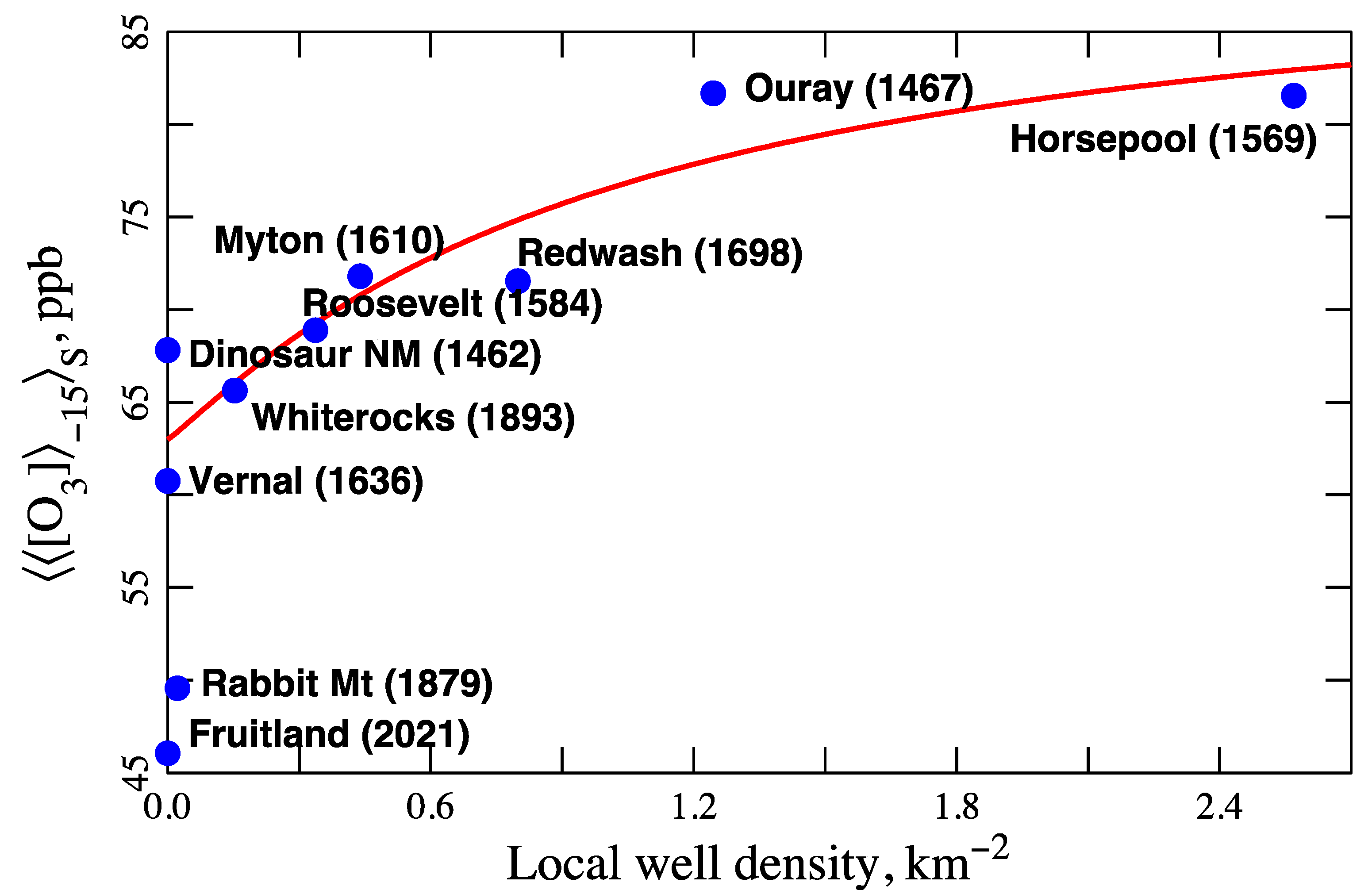
3.6. Impact of Proximity to Well Pads

Ten measurement sites provide data over all seasons from 2011 to 2019. Let ${\langle {\langle \left[{\mathrm{O}}_3\right]\rangle }_{-15}\rangle }_S$ represent the average of ${\langle \left[{\mathrm{O}}_3\right]\rangle }_{-15}$ over the snow seasons between 2011 and 2019. It therefore represents the long-term average ozone concentration at any particular site when lapse rates are about −15 K/km and snow is on the ground. The local well density is defined as the number of well pads per km² within a ten-kilometer radius of the measurement site. Figure 9 demonstrates that ozone concentrations are correlated with this local density. Proximity to well pads is a strong predictor of ozone concentration. The two outliers, Rabbit Mountain and Fruitland, lie at higher elevations, and can be expected to have lower ozone concentrations.

3.7. Interannual Trends in Ozone Precursor Concentrations

Downward trends in ozone precursor emissions and concentrations are the most likely explanation for the downward trend in ozone. This section presents an analysis of interannual trends in winter season-average ozone precursor concentrations. We used the season averages of (1) all available data, (2) data from days when the pseudo-lapse rate was above zero (to eliminate bias caused by precursor buildup during inversion episodes), and (3) precursor concentrations multiplied by wind speed (to account for the effects of wind speed on concentrations) on days when the pseudo-lapse rate was above zero. All three methods showed similar interannual trends, but method 2 resulted in less interannual variability (i.e., smoother trends). We present the results of method 2 here.

Figure 10 shows the seasonal average NO_x concentrations at all sites with available data along with medians for each season. The mean of the medians over the last four seasons (2017–2020) is only 58% of the mean over the first four seasons (2010–2013). The four highest medians occurred in the first four years, 2010–2013. At all sites but Whiterocks and Vernal, the averages over 2017–2020 are between 42% and 74% of averages over 2010–2013. Vernal saw an even larger decline to 38%, probably because the Vernal monitoring station moved in 2015 to a site more removed from possible NO_x sources (from near a busy highway and airport to the edge of the metropolitan area). Whiterocks saw a decline to only 91%, but NO_x there is consistently low. The correlation between NO_x and time is negative at all sites. The trend line through the medians has slope −0.32 ± 0.10 (95% confidence interval) ppb/season and Pearson’s R² = 0.79.

Organic compound data have only consistently been collected at the Horsepool and Roosevelt sites. The collection and analysis methods changed over time, with real-time GC through 2015, and three-hour once-daily (beginning at midnight or noon MST) whole-air canister samples thereafter. Figure 11 shows that average concentrations of total non-methane hydrocarbons (TNMHC), ethane, and toluene have all declined since 2012 or 2013, but have rebounded in recent years. TNMHC and ethane in Roosevelt declined in 2018 to about 20% to 50% of the initial 2013 value, and then rebounded to about 50% to 90% in 2020. At Horsepool, TNMHC and ethane declined in 2018 and 2019 to about 30% to 50% of the 2012 value, and then recovered to about 50% to 90% in 2020. Toluene was present at both sites at concentrations of only about 1–2 ppb. It also passed through a minimum and then rebounded to about 85% to 165% of the 2012 or 2013 value.

3.8. Tests of Statistical Significance

One test of statistical significance of timeline trends is to calculate confidence intervals for the slopes.

Table 2. 95% confidence intervals for the slopes of several trend lines.

Trend Line	Slope with Confidence Interval
Ozone exceedance count, Figure 3	−3.8 ± 1.7 counts per year
${\langle \left[{\mathrm{O}}_3\right]\rangle }_{-15},$Figure 8	−3.0 ± 2.0 ppb per year
NOx medians, Figure 10	−0.32 ± 0.10 ppb per year

summarizes results for the trend lines in Figure 3, Figure 8 and Figure 10. Zero slope lies outside the confidence intervals, indicating that all three slopes are non-zero with better than 95% confidence.

Table 3. Results of tests of statistical significance: The probability that the indicated occurrence could have occurred at random.

OCCURENCE	p
Three seasons with no snow out of 11 total were the same three seasons to have low ozone, Figure 2.	${\frac{3!8!}{11!}}_{}^{}\cong 0.006$
Figure 2, Figure 3 and Figure 8 all display some metric of ozone levels; the three largest values of the metric occur in the first three out of eight snow seasons.	${\frac{3!5!}{8!}}_{}^{} \cong 0.018$
The first four NOx seasons out of 11 total were the same to display the four largest medians, Figure 10.	${\frac{4!7!}{11!}}_{}^{} \cong 0.003$
The medians over the eight snow seasons in Figure 8 are sufficiently ordered to trend downward at least as steeply as −3 ppb/year.	≅ 0.015
The medians over the 11 seasons in Figure 10 are sufficiently ordered to trend downward at least as steeply as −0.325 ppb/year.	≅ 0.0003

summarizes several p-tests that have been applied to the data. p represents the probability that the indicated occurrence or null hypothesis could have occurred randomly. For the first three occurrences, p is determined by combinatorics. For the remaining two, p was determined by Monte Carlo calculations in which we scrambled the x-coordinates of all points, and then computed the probability that any least-squares line is at least as steep as the line through the unscrambled data. The p values are all much lower than the threshold, 0.05, traditionally cited as the indicator for statistical significance. They all indicate that the trends observed in Figure 2, Figure 3, Figure 8 and Figure 10 are statistically significant.

3.9. Trends in the Oil and Natural Gas Industry

The data indicate that winter ozone in the Uinta Basin has been declining since it was first measured in 2010. There are probably two causes for the decline: (1) a decrease in global demand for oil and natural gas has led to decreased industrial activity; and (2) many pollution controls have come online over the last decade. At the time of writing this, we have no way of knowing the relative importance of either cause.

Global market forces drive fossil fuel production. Price increases led to an increase in drilling [28], wells, and oil and gas production in the Uinta Basin until 2014 [26] (Figure 12). A price collapse after 2014 caused a rapid decline in drilling, which led to a leveling-off and then a slow decline in the number of producing wells in the Basin. Oil production peaked in 2015 and, after a drop in 2016 and 2017, has been steady at about 375 million L/month from 2018 through 2020, 70% higher than the 2010–2012 average. Gas production has steadily declined from a peak of about $8 \times {10}^8{\mathrm{m}}^3/\mathrm{month}$ in 2010–2012 to only 64% of that in 2018–2020.

Drilling is an important source of NO_x, while the production of oil and gas is linked to both NO_x and organic emissions. The data suggest that the decline in ozone precursor concentrations may be linked in part to the declines in drilling or to gas production.

3.10. Pollution Controls

Pollution controls at oil and gas wells, either mandated by government regulation or installed voluntarily by owners, have increased over the last decade. In 2012 the U.S. Environmental Protection Agency (EPA) issued Code of Federal Regulations (CFR) 40, Part 60, Subpart OOOO (a.k.a., Quad-O), which regulates organic compound emissions from oil and gas facilities [29,30,31]. It was implemented in a phased approach between October 2012 and October 2015. Quad-O regulations only apply to facilities constructed or modified after the implementation dates. In total, 85% of oil and gas wells in the Uinta Basin were completed before October 2013, when the first of the Quad-O provisions that affect well-site operations took effect. Seventy-seven percent of the wells completed since October 2013 are oil wells.

EPA issued a separate rule in 2012 restricting emissions of hazardous air pollutants from glycol dehydrators to a total of less than 25 tons/year [29,30]. This rule applied to new and existing dehydrators, and was phased in between 2012 and 2015. An emissions inventory developed by the Utah Division of Air Quality for the year 2014 showed that, of 1904 glycol dehydrators in the Uinta Basin, only 0.2% had emissions of total volatile organics greater than 25 tons/year [32]. Thus, we assume this rule had a small impact on emissions of ozone-forming organics in the Uinta Basin.

Additional regulation promulgated by EPA in 2016 (CFR 40, Part 60, Subpart OOOOa; a.k.a., Quad-Oa) requires companies that construct new oil and gas facilities to inspect those facilities for natural gas leaks periodically (usually semiannually), and to repair leaks that are found [31]. Even though Quad-Oa only applies to new or modified facilities, in a survey of Uinta Basin oil and gas producers conducted in 2018 by Lyman et al. [33], 83% of respondents indicated they inspected all oil and gas wells at least annually. The same study showed that when one company implemented a leak detection and repair program that was more aggressive than EPA requirements, along with upgraded emissions control equipment, detection of emission plumes at that company’s wells dropped by 79%.

The Utah Division of Air Quality has also adopted standards to control organic compound emissions from oil and gas wells [34]. These standards are either the same as, or similar to, Quad-O and Quad-Oa regulations.

4. Discussion and Conclusions

At neutral atmospheric conditions, $\mathsf{\Psi }\approx 9 \mathrm{K}/\mathrm{km}$ [27], ozone tends to be near the background value of about 40 ppb, during seasons both with and without snowpacks. Under inversion conditions, $\mathsf{\Psi }\approx -15 \mathrm{K}/\mathrm{km}$, and when a snowpack is present, ozone concentrations are above background, depend on proximity to oil and gas wells, and decrease over time. Under inversion conditions, $\mathsf{\Psi }\approx -15 \mathrm{K}/\mathrm{km}$, and in the absence of a snowpack, ozone concentrations are below background and appear to be increasing over time. The most logical explanation is that compounds responsible for ozone production when the actinic flux is high (NO_x and organics), and for ozone reduction when the actinic flux is low (NO_x), have been decreasing.

Indeed, trends in ozone precursors have paralleled the decrease in ozone over the previous decade. Ozone and NO_x concentrations at all sites have been trending down at the rate of about 3 and 0.3 ppb/year, respectively. Average ozone concentrations over the three-year period 2017, 2019, and 2020 are only about 67% of the concentrations over the period 2010, 2011, and 2013. Average NO_x concentrations over the period 2018–2020 are 58% of those over 2010–2012. Average concentrations of organics fell in 2018 to about 40% of their 2012 or 2013 values. The concentration of organics has shown an upturn in recent years, due perhaps to new sources that have come online recently. Several p-tests indicate that the declines in ozone and NO_x are statistically significant.

Several years ago, we drew comparisons between the Uinta Basin of Utah and the Upper Green River and Wind River Basins of Wyoming [9]. All three basins experience persistent inversions, snowpacks, and are home to oil or natural gas extraction. The Upper Green and the Wind River Basins are at comparable latitudes and therefore see the same solar elevation. However, high winter ozone occurs in the Uinta and Upper Green River Basins, but not in the Wind River Basin, presumably because oil or gas production there is lower. This suggests that there is a threshold for oil and gas emissions above which high ozone begins to occur, but below which ozone remains at background levels. The two trend lines in Figure 8 are converging, indicating that the Uinta Basin may be approaching that threshold.

A number of authors have presented evidence that the Uinta Basin ozone system is NO_x-limited [17,35]. Insensitivity to the recent upturn in organics emissions may also be an indication of NO_x control.

We believe that there are two causes for the decrease in ozone precursor concentrations. First, declines in the global demand for oil and natural gas have led to a decrease in oil and gas extraction activity. Second, government-mandated and voluntary pollution controls have come online since 2010 (Section 3.10). However, these controls only targeted emissions of organics. They cannot explain the decline in NO_x concentrations. The trends in well-drilling or gas production documented in Figure 12 may explain the NO_x decline.

The trend line in Figure 3 reaches zero exceedance days per season in 2020. The trend line in Figure 8 has been below 70 ppb since 2014, and is converging on background ozone levels. These are encouraging trends, but there could very well be a resurgence of winter ozone if fossil fuel extraction activity increases in the Basin.

References

1. Schnell, R.C.; Oltmans, S.J.; Neely, R.R.; Endres, M.S.; Molenar, J.V.; White, A.B. Rapid photochemical production of ozone at high concentrations in a rural site during winter. Nat. Geosci. 2009, 2, 120–122. [Google Scholar] [CrossRef]
2. Martin, R.; Moore, K.; Mansfield, M.; Hill, S.; Harper, K.; Shorthill, H. Uinta Basin Winter Ozone and Air Quality Study. 2011. Available online: https://binghamresearch.usu.edu/files/edl_2010-11_report_ozone_final.pdf (accessed on 15 October 2020).
3. Lyman, S.; Shorthill, H. 2012 Uintah Basin Winter Ozone & Air Quality Study. 2013. Available online: Binghamresearch.usu.edu/files/ubos_2011-12_final_report.pdf (accessed on 15 October 2020).
4. Lyman, S.; Mansfield, M.; Shorthill, H. 2013 Uintah Basin Winter Ozone & Air Quality Study. 2013. Available online: https://binghamresearch.usu.edu/files/2013%20final%20report%20uimssd%20R.pdf (accessed on 16 October 2020).
5. Lyman, S.; Shorthill, H.; Mansfield, M.; Tran, H.; Trang, T. 2013–14 Uintah Basin Winter Ozone Study. 2014. Available online: Binghamresearch.usu.edu/files/UBOS_2014_FinalReport_.pdf (accessed on 15 October 2020).
6. Oltmans, S.; Schnell, R.; Johnson, B.; Petron, G.; Mefford, T.; Neely, R., III. Anatomy of wintertime ozone associated with oil and natural gas extraction activity in Wyoming and Utah. Elem. Sci. Anthr. 2014, 2, 000024. [Google Scholar] [CrossRef] [Green Version]
7. Field, R.A.; Soltis, J.; McCarthy, M.C.; Murphy, S.; Montague, D.C. Influence of oil and gas field operations on spatial and temporal distributions of atmospheric non-methane hydrocarbons and their effect on ozone formation in winter. Atmospheric Chem. Phys. Discuss. 2015, 15, 3527–3542. [Google Scholar] [CrossRef] [Green Version]
8. Lyman, S. 2014–2015 Uintah Basin Winter Ozone Study. 2015. Available online: binghamresearch.usu.edu/files/UBOS_2015_FinalReport.pdf (accessed on 16 October 2020).
9. Mansfield, M.L.; Hall, C.F. A survey of valleys and basins of the western United States for the capacity to produce winter ozone. J. Air Waste Manag. Assoc. 2018, 68, 909–919. [Google Scholar] [CrossRef] [PubMed]
10. Mansfield, M.L.; Hall, C.F. Statistical analysis of winter ozone events. Air Qual. Atmos. Health 2013, 6, 687–699. [Google Scholar] [CrossRef]
11. Mansfield, M.L. Statistical analysis of winter ozone exceedances in the Uintah Basin, Utah, USA. J. Air Waste Manag. Assoc. 2018, 68, 403–414. [Google Scholar] [CrossRef] [PubMed] [Green Version]
12. US Environmental Protection Agency, Air Quality System (AQS) API. Available online: https://aqs.epa.gov/aqsweb/documents/data_api.html (accessed on 23 September 2020).
13. Dunlea, E.J.; Herndon, S.C.; Nelson, D.D.; Volkamer, R.M.; Martini, F.S.; Sheehy, P.M.; Zahniser, M.S.; Shorter, J.H.; Wormhoudt, J.C.; Lamb, B.K.; et al. Evaluation of nitrogen dioxide chemiluminescence monitors in a polluted urban environment. Atmos. Chem. Phys. Discuss. 2007, 7, 2691–2704. [Google Scholar] [CrossRef] [Green Version]
14. Sadanaga, Y.; Fukumori, Y.; Kobashi, T.; Nagata, M.; Takenaka, N.; Bandow, H. Development of a Selective Light-Emitting Diode Photolytic NO2Converter for Continuously Measuring NO2in the Atmosphere. Anal. Chem. 2010, 82, 9234–9239. [Google Scholar] [CrossRef] [PubMed]
15. Villena, G.; Bejan, I.; Kurtenbach, R.; Wiesen, P.; Kleffmann, J. Interferences of commercial NO2 instruments in the urban atmosphere and in a smog chamber. Atmos. Meas. Tech. 2012, 5, 149–159. [Google Scholar] [CrossRef] [Green Version]
16. Lyman, S.; Mansfield, M.; Tran, H.; Trang, T. 2018 Annual Report: Uinta Basin Air Quality Research. 2018. Available online: https://usu.box.com/s/rigadr7yt7ipir4gzj75vfaazoe8u8mt (accessed on 9 November 2020).
17. Edwards, P.M.; Young, C.J.; Aikin, K.; De Gouw, J.A.; Dubé, W.P.; Geiger, F.; Gilman, J.; Helmig, D.; Holloway, J.S.; Kercher, J.; et al. Ozone photochemistry in an oil and natural gas extraction region during winter: Simulations of a snow-free season in the Uintah Basin, Utah. Atmos. Chem. Phys. Discuss. 2013, 13, 8955–8971. [Google Scholar] [CrossRef] [Green Version]
18. Edwards, P.M.; Brown, S.S.; Roberts, J.M.; Ahmadov, R.; Banta, R.M.; Degouw, J.A.; Dubé, W.P.; Field, R.A.; Flynn, J.H.; Gilman, J.B.; et al. High winter ozone pollution from carbonyl photolysis in an oil and gas basin. Nat. Cell Biol. 2014, 514, 351–354. [Google Scholar] [CrossRef] [PubMed]
19. Stoeckenius, T.; McNally, D. (Eds.) Final Report: 2013 Uinta Basin Winter Ozone Study. 2014. Available online: https://binghamresearch.usu.edu/files/UBOS_2013_Final_Report_-_PDF.zip (accessed on 15 October 2020).
20. Stoeckenius, T. Final Report: 2014 Uinta Basin Winter Ozone Study. 2015. Available online: http://binghamresearch.usu.edu/files/UBWOS_2014_Final.pdf (accessed on 16 October 2020).
21. Lyman, S.; Mansfield, M.; Tran, H.; Trang, T.; Holmes, M. 2019 Annual Report: Uinta Basin Air Quality Research. 2019. Available online: https://usu.box.com/s/co626elackqkw9ead14wkma14jjv9eng (accessed on 16 October 2020).
22. Lyman, S.; Mansfield, M.; Trang, H.; Tran, T. Management Plan: Uinta Basin Air Quality Research. 2020. Available online: https://usu.box.com/s/877z4o8nwynu3uwcze8uxj8jaant7auw (accessed on 10 October 2020).
23. Lyman, S.; Mansfield, M.; Tran, H.; Trang, T. Annual Report: Uintah Basin Air Quality Research Project. 2016. Available online: https://binghamresearch.usu.edu/files/UBAQRS_Nov2016_AnnualReport.pdf (accessed on 15 October 2020).
24. Lyman, S.; Mansfield, M.; Tran, H.; Tran, T. Annual Report: Uintah Basin Air Quality Research. 2017. Available online: https://usu.app.box.com/s/7bd8f3hjs3u0pa7tefl6etue3e2ol4tj (accessed on 17 October 2020).
25. Utah Climate Center. Available online: https://climate.usu.edu/mapGUI/mapGUI.php (accessed on 28 June 2020).
26. Utah Division of Oil, Gas, and Mining, Data Research Center. Available online: https://oilgas.ogm.utah.gov/oilgasweb/data-center/dc-main.xhtml (accessed on 16 October 2020).
27. Seinfeld, J.H.; Pandis, S.N. Atmospheric Chemistry and Physics: From Air Pollution to Climate Change; Wiley-Interscience: Hoboken, NJ, USA, 2006; Volume 2, p. 724. [Google Scholar]
28. Baker-Hughes, North America Rig Count. Available online: https://bakerhughesrigcount.gcs-web.com/na-rigcount?c=79687&p=irolreportsother%20%3erigs%20by%20state%20current%20and%20historical%20%20this%20is%20the%20rig%20count%20for%20the%20whole%20state (accessed on 12 October 2020).
29. Carbonell, T. EPA Issues Final Emission Standards for Oil and Gas Sector. 2012. Available online: https://www.vnf.com/webfiles/VNF_Alert_4-20-12.pdf (accessed on 12 October 2020).
30. Healey, B.; Pergande, K. Breaking down Quad-O regulations, compliance needs. Pipeline Gas J. 2014, 241, 90–94. [Google Scholar]
31. Federal Register, Environmental Protection Agency. Oil and Natural Gas Sector: Emission Standards for New, Reconstructed, and Modified Sources. Available online: https://www.gpo.gov/fdsys/pkg/FR-2016-06-03/pdf/2016-11971.pdf (accessed on 14 October 2020).
32. Utah Division of Air Quality, 2014 Air Agencies Oil and Gas Emissions Inventory: Uinta Basin. Available online: https://deq.utah.gov/air-quality/2014-air-agencies-oil-and-gas-emissions-inventory-uinta-basin (accessed on 18 October 2020).
33. Lyman, S.N.; Tran, T.; Mansfield, M.L.; Ravikumar, A.P. Aerial and ground-based optical gas imaging survey of Uinta Basin oil and gas wells. Elem. Sci. Anth. 2019, 7, 43. [Google Scholar] [CrossRef]
34. Utah Division of Air Quality, Centralized Air Emissions Reporting System. Available online: https://deq.utah.gov/air-quality/centralized-air-emissions-reporting-system (accessed on 12 October 2020).
35. Womack, C.C.; McDuffie, E.E.; Edwards, P.M.; Bares, R.; de Gouw, J.A.; Docherty, K.S.; Dubé, W.P.; Fibiger, D.L.; Franchin, A.; Gilman, J.B.; et al. An Odd Oxygen Framework for Wintertime Ammonium Nitrate Aerosol Pollution in Urban Areas: NOx and VOC Control as Mitigation Strategies, Geophysical Research Letters. Soil Water Clim. 2019, 46, 4971–4979. [Google Scholar]
Figure 1. Difference between NO2 measured with an instrument utilizing a molybdenum oxide NO2 converter and NO2 measured with an instrument utilizing a UV photolytic converter versus NOz at the Roosevelt monitoring station. The black line shows a linear regression curve for the relationship. From [16].
Atmosphere 12 00004 g001
Figure 2. Seasonal average of the daily maximum in the 8-h running average ozone concentration at Ouray, Utah and basin-average snow depth, over the months of January and February, for each of the 11 indicated winter seasons.
Atmosphere 12 00004 g002
Figure 3. Seasonal ozone exceedances of the current National Ambient Air Quality Standard for ozone at the Ouray site. Seasons with and without snow cover are blue and red, respectively. The trend line for the seasons with snow cover is plotted and has the indicated slope and correlation coefficient.
Atmosphere 12 00004 g003
Figure 4. Histograms of the distribution of the daily pseudo-lapse rate, distinguishing seasons without snow (2012, 2015, 2018) from seasons with snow (2010, 2011, 2013, 2014, 2016, 2017, 2019, 2020).
Atmosphere 12 00004 g004
Figure 5. When a snowpack is absent, ozone concentration and pseudo-lapse rate at a given site are almost always positively correlated (left). When a snowpack is present, they are almost always negatively correlated (right). Least-squares trend lines are shown in blue.
Atmosphere 12 00004 g005
Figure 6. Out of 177 available pairings of measurement sites and measurement seasons, the overwhelming majority (gray and green bars) fit a pattern: Negative correlation between ozone concentration and lapse rate (down arrows) when snow is present, and positive correlation (up arrows) when snow is not present. Only 5% of the 177 instances (blue and red bars) do not fit this pattern. Two-thirds of the pattern violations occur at sites above about 2000 m (a) and all occur with small correlation coefficients (b).
Atmosphere 12 00004 g006
Figure 7. Black lines are trend lines from the ozone concentration vs. pseudo-lapse rate plots for any given season and for the Ouray site. Usually, the trend lines radiate outward from a convergence region (vicinity of the blue circle). The vertical red line at Ψ = 15   K / km is used to define [ O 3 ] 15 , i.e., the value of each trend line when Ψ = 15   K / km . Horizontal red lines guide the eye to indicate the corresponding season.
Atmosphere 12 00004 g007
Figure 8. Box–whisker plots of the distribution of [ O 3 ] 15 over all sites in any given season. Whiskers extend from the minimum to the maximum; boxes extend from the 25th to the 75th percentile with medians also shown. Each box is labeled with the number of sites in any given season. Only two datapoints are available in 2010, so a box–whisker construction is not possible. Blue and red designate seasons with and without snow, respectively. The upper dashed line has slope = −3.0 ± 2.0 (95% confidence interval) ppb/season, and Pearson’s R2 = 0.61. It represents the trend line drawn through the medians of seasons with snow. The lower dashed line (slope = +1.8 ppb/season, R2 = 0.65) is the trend line for seasons without snow.
Atmosphere 12 00004 g008
Figure 9. Plot of [ O 3 ] 15 S , representing the long-term average ozone concentration when the lapse rate is ca. −15 K/km and when a snowpack is present, vs. local well density at ten measurement sites. Numbers in parentheses are the elevations (m) of each site. The red trace is a suggested correlation curve.
Atmosphere 12 00004 g009
Figure 10. Winter season average NOx from Uinta Basin monitoring stations. Only data from days with a pseudo-lapse rate above zero are included. Data shown are the average of each site. The medians taken over all sites in each single season and the trend line through these medians are also shown. The trace for Vernal is broken because the monitoring site moved in 2015 to a site more distant from possible NOx sources.
Atmosphere 12 00004 g010
Figure 11. Time-line plots of the average winter-time concentrations of TNMHC, ethane, and toluene. Whiskers show the 95% bootstrap confidence intervals of each mean. Selected datapoints are labeled in red with the ratio of the mean concentration in the indicated season to the mean concentration in the initial season; subscripts and superscripts give the limits of the 95% bootstrap confidence intervals of each ratio.
Atmosphere 12 00004 g011
Figure 12. Number of producing oil and gas wells, total natural gas production, and total oil production in the Uinta Basin for the month of February of the indicated season. Average number of drilling rigs in the state of Utah each February is also shown.
Atmosphere 12 00004 g012