Article

Estimation of the Grassland Aboveground Biomass of the Inner Mongolia Plateau Using the Simulated Spectra of Sentinel-2 Images

1
Key Laboratory of 3D Information Acquisition and Application, Capital Normal University, Ministry of Education, Beijing 100048, China
2
Engineering Research Center of Spatial Information Technology, Capital Normal University, Ministry of Education, Beijing 100048, China
3
Key Laboratory of Ecosystem Network Observation and Modeling, Institute of Geographic Sciences and Natural Resources Research, Chinese Academy of Science, Beijing 100101, China
4
School of Life Science, Shanxi University, Taiyuan 030006, China
*
Author to whom correspondence should be addressed.
Remote Sens. 2020, 12(24), 4155; https://doi.org/10.3390/rs12244155
Submission received: 9 October 2020 / Revised: 15 December 2020 / Accepted: 16 December 2020 / Published: 18 December 2020

Abstract

:
An accurate assessment of the grassland aboveground biomass (AGB) is important for analyzing terrestrial ecosystem structures and functions, estimating grassland primary productivity, and monitoring climate change and carbon/nitrogen circulation on a global scale. Multispectral satellites with wide-width advantages, such as Sentinel-2, have become the inevitable choice for the large-scale monitoring of grassland biomass on regional and global scales. However, the spectral resolution of multispectral satellites is generally low, which limits the inversion accuracy of grassland AGB and restricts further application in large-scale grassland monitoring. For this reason, a satellite-scale simulated spectra method was proposed to enhance the spectral information of the Sentinel-2 data, and a simulated spectrum (SS) was constructed using this algorithm. Then, the raw spectrum (RS) of Sentinel-2 and the SS were used as data sources to calculate the vegetation indices (RS-VIs and SS-VIs, which represent vegetation indices calculated using RS and SS data, respectively), and the multi-granularity spectral segmentation algorithm (MGSS) was employed to extract spectral segmentation features (RS-SF and SS-SF, which represent segmentation features extracted by RS and SS data, respectively). Following this, these spectral features (RS-SF, SS-SF, RS-VIs, and SS-VIs) were used to estimate AGB by partial least-squares regression (PLSR) and multiple stepwise regression (MSR) models. Finally, the spatial distribution law and the reasons for the latitude zone of the Inner Mongolia Plateau were analyzed, based on precipitation, the average temperature, topography, etc. The conclusions are as follows. Firstly, the SS has more spectral information and its sensitivity to biomass is higher than the RS of Sentinel-2 in some bands, and the correlation between the SS-VIs and biomass is higher than that of the RS-VIs. Secondly, among the spectral features, the most accurate AGB estimation was obtained by SS-SF, which gave R2 = 0.95. The root mean square error (RMSE) was 10.86 g/m2 and the estimate accuracy (EA) was 82.84% in the MSR model. Additionally, RMSE = 10.89 g/m2 and EA = 82.78% in the PLSR model. Compared with the traditional estimation methods using RS and VI, R2 was increased by at least 0.2, RMSE was reduced by at least 14.08 g/m2, and EA was increased by 22.26%. Therefore, the simulated spectra method can help improve the estimation accuracy of AGB, and a new idea about regional and global large-scale biomass acquisition is provided.

Graphical Abstract

1. Introduction

Aboveground biomass (AGB) refers to the mass of plant organic matter per unit area, which is a key trait indicating plant health and ecosystem function [1]. Grassland, as one of the most widely distributed terrestrial ecosystem types in the world, accounts for 26% of the global land surface area [2]. Timely and accurate monitoring of AGB changes in grasslands is of great significance for maintaining the terrestrial ecosystem structure and function, maintaining the balance of vegetation productivity and surface energy, monitoring the carbon/nitrogen circulation of global ecosystems, and global climate change [3].
Traditional manual methods of measuring AGB, which include field collection and measurement in the laboratory, cause great damage to vegetation. Moreover, it is difficult to obtain AGB data due to their time- and labor-consuming approaches on a large-scale, which cannot meet the needs of scientific research [4]. Remote sensing provides a non-destructive, more efficient and convenient, and time-continuous biomass survey method [5]. The plant physiological structure, chemical composition, and environmental stress (water, salt, temperature, etc.) have an impact on the reflectivity of leaves and the canopy. Therefore, information such as the chlorophyll, C, N, and P content and AGB can be obtained according to spectral characteristics [6,7]. The methods of estimating AGB based on remote sensing are mainly divided into physically-based models and empirical regression techniques [8]. Physically-based models (such as SAIL, PROSPECT, PROSAIL, etc.) consider plant leaf structural parameters, the chlorophyll content, the leaf area index, soil factors, and other factors [9] to simulate AGB, but various parameters in these models are often not readily available, which limits the applicability of physical models. There is a strong correlation between the vegetation index and biomass in NDVI [10], and the empirical regression techniques based on that correlation relationship have become a common means to estimate AGB [11,12]. For example, Cabrera-Bosquet et al. [13] used NDVI to successfully estimate the wheat biomass and nitrogen content, and improved the efficiency of genetic breeding. Furthermore, Wang et al. [14] calculated the NDVI, RVI, GNDVI, EVI, SAVI, etc., vegetation indexes based on HJ-CCD images, and then used the random forest regression algorithm to estimate the biomass of wheat in South China, greatly reducing the estimated cost of biomass.
Although remote sensing technology can efficiently estimate AGB, the selection of reasonable remote sensing data can reduce the biomass estimation error and biomass estimation cost. Commonly used remote sensing platforms are airborne and spaceborne UAV, which can be flexibly equipped with a variety of hyperspectral cameras; have the advantages of a high spatial resolution, spectral resolution, and temporal resolution [15,16]; and play an important role in the field of precision agriculture, such as in crop yield estimation [17], growth monitoring [18], and genetic breeding [19,20]. However, the endurance of UAV and other airborne platforms greatly limits the acquisition of airborne hyperspectrum, multispectrum, and other data. In addition, in large-scale grassland monitoring, there is still a reliance on satellite (hyperspectrum and multispectrum) means to monitor the ground. Compared with multispectral satellites, hyperspectral satellites have relatively few types, narrow widths, and high prices, so are also difficult to apply on large scales [21]. Dube et al. [22] compared the ability of ETM+ and OLI to invert AGB, and concluded that the medium-scale resolution satellite Landsat8 has a higher precision in biomass prediction on a regional scale. Li et al. [23] used Landsat8 and Sentinel-2 images to successfully predict the chlorophyll content (CHL) and dry matter content (DMC) of alpine grassland in Tibet, China. These examples show that multispectral satellites have great potential in biomass prediction on a large scale. It is undeniable that multispectral images lack spectral detail information compared to hyperspectral data, which affects the prediction accuracy of plant traits. Immitzer et al. [24] classified farms and forests and identified species with Sentinel-2 data, and the cross-validation results showed that the accuracy of crop type identification was 76%, while the accuracy of tree species identification only reached 65%. Ustin et al. [25] argue that the relationship between vegetation traits and reflectivity is reduced when the leaf scale is extended to the canopy scale, and Schaepman [26] and Vohland [27] believe that there are uncertainties with regards to the inversion accuracy of AGB on the canopy scale due to the canopy structure and observation angle. Therefore, enhancing image spectral detail information is an effective way of improving the accuracy of grassland traits such as biomass when using multispectral satellites with a wider range and lower resolution to monitor grassland.
Improving the ability of the multispectral satellite to invert biomass has become a hot spot in the accurate estimation of grassland biomass on a large scale. At present, there are three main directions for improving the accuracy of biomass estimation: (i) combining vegetation index and physiological structure parameters to estimate biomass, such as the grass height and image texture [8,28,29]; (ii) combination with other data sources, such as SAR [30]; and (iii) enhancing the sensitivity of the vegetation index to AGB. The application of image texture features in forestry and precision agriculture improves the prediction accuracy of biomass [31], but the grassland and woodland have different structural features, the height of the grass is relatively low, and the grass canopy is uniform. In medium-scale resolution images, the grass texture features become inconspicuous, and it is difficult to obtain centimeter-level grass height data or digital elevation model (DEM) information. The contribution rate of grassland texture features to biomass inversion under large-scale conditions is still unclear and requires further exploration; SAR is suitable for all-weather ground monitoring, even on rainy days. Combining SAR data with the vegetation index can reduce the saturation problem of the vegetation index in high coverage areas and improve the estimation accuracy of biomass [32]. However, it is expensive and not suitable for large-scale grassland monitoring needs. The estimation accuracy of AGB can be improved by constructing the narrow-band hyperspectral vegetation index [8]. The spectral index (NDVI, etc.) constructed by wide-band satellites will have saturation problems in high vegetation coverage areas, which increases the difficulty of biomass inversion, while the narrow-band vegetation index can effectively alleviate the shortage of the wide-band vegetation index [33], so it is mostly achieved by replacing the multispectrum with the hyperspectrum. Furthermore, the use of continuous wavelet decomposition, spectral segmentation, and fractional differential methods can also enhance the sensitivity of the spectrum to some extent [34,35,36], in order to improve the accuracy of the model. However, multispectral satellites are limited by wavelength and wave width, and it is difficult to directly construct a narrow-band vegetation index and derivative analysis. How to construct derivative spectra suitable for multispectral satellites is key to further improving the accuracy of large-scale biomass inversion.
In recent years, the Mongolian Plateau has been affected by global warming, increased evaporation, and decreased precipitation, and the grassland ecosystem has degraded. It is a sensitive area of the northern grassland under global climate change [37]. The timely monitoring AGB is of great significance in monitoring global climate change, and the protection of grassland ecosystems is of great significance. The objectives of this study are to propose a satellite-scale simulated spectral method to improve the ability of multispectral satellites to obtain AGB on a large scale, and to evaluate the accuracy of the results. This article is mainly divided into three parts: (i) a simulated spectral method is proposed to improve the spectral information of Sentinel-2 images; (ii) spectral features related to biomass, the raw spectrum, and the simulated spectrum are extracted; segmentation features are extracted by the multi-granularity spectral segmentation algorithm, wide-band vegetation index, and narrow-band vegetation index; and partial least-squares regression (PLSR) and multiple stepwise regression (MSR) biomass estimation models are established; and (iii) the best model for estimating the AGB, evaluating the accuracy, and mapping the biomass distribution is selected.

2. Materials and Methods

2.1. Study Area

The study area (Figure 1, 109–125°E, 43.5–45.3°N) is located in the central part of the Inner Mongolia Autonomous Region and western Jilin Province, with an altitude of 140–1300 m. It belongs to a temperate continental climate, with a high temperature and rain in summer, and cold and dry winter. Precipitation gradually decreases from east to west, mainly across typical temperate grasslands, meadow grasslands, and desert grasslands. The dominant species in this area are Stipa, Leymus, Artemisia frigida, Codonopsis, and Potentilla [38].

2.2. Datasets

2.2.1. Field Data

The field measurements were collected from 3–14 July 2018, at the growth peak of the grasslands. To investigate the AGB of grassland in the Inner Mongolia Plateau, 10 sampling areas were established from east to west, each with an area of about 0.5 ha. Each sampling area produced eight samples, resulting in a total of 80 sampling points, and the distribution of sampling points is shown in Figure 1. All sampling points were scattered, and the distance between the sampling points was in the range of 15–55 m, so that the sampling points corresponded to the Sentinel-2 (10 m) pixels. Each sampling point was set to a 1 × 1 m2, and after the ASD spectrometer had acquired the sample spectrum, the quadrat was harvested in the full pasture, labeled in bags, and refrigerated, and the center position of each sampling point was recorded by GPS. The dry matter content was measured after 48 h of drying in the oven at 65 °C in the laboratory.
The field grassland canopy hyperspectral reflectance was measured by using a field spectrometer (ASD Field Spec 2 spectrometer, Analytical Spectral Devices, Boulder, CO, USA). The ASD spectrometer can provide uniform visible near-infrared (325–1075 nm) data, a spectral resolution <3.0 nm, and a field of view angle of 25°. Before the measurement, the whiteboard matched with the instrument was used to calibrate the ASD radiation and convert the ASD to the relative reflectance mode. Under clear sky conditions between 10:00 and 14:00, at a height of 1.3 m above the ground (the coverage of the spectrometer on the ground is about 0.26 m2), the pure spectrum of bare soil and grass which had a coverage of more than 95% was measured, and the measurement was repeated three times for each point, with the average value being taken as the final reflectance.

2.2.2. Remote Sensing Data
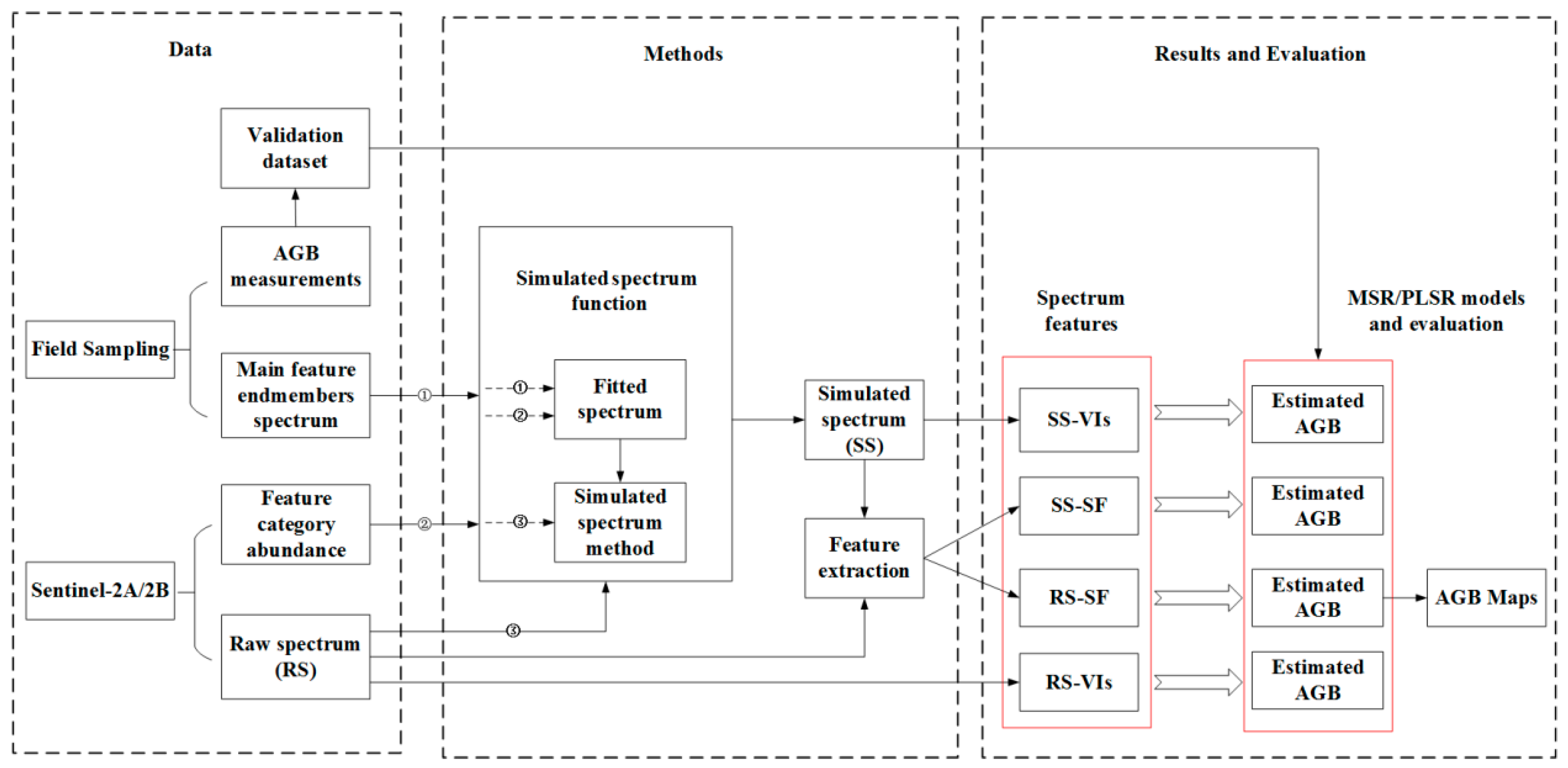
Sentinel-2 is becoming increasingly used in environmental monitoring. Sentinel-2A was successfully launched in 2015 with a width of 295 km and the spatial resolution is divided into three levels of 10, 20, and 60 m. Sentinel has a higher time resolution, and it can achieve repeated observations in the same area for 5 days, in cooperation with Sentinel-2B. It has 13 bands of the visible to short-wave infrared range, and three “red-edge” bands are set at 705–783 nm for vegetation reflectance characteristics [39]. The spatial and temporal resolution of Sentinel-2 is better than Landsat 8, so Sentinel-2A/B images were selected as the data source. Limited by conditions such as the sampling time and cloud occlusion, nine scenes of Sentinel-2 images were downloaded from the European Space Agency ESA (website: https://scihub.copernicus.eu/dhus/#/home) and the image acquisition time was between 1 July and 13 July. There was no suitable image for the S2 sampling area. The images were pre-processed by SNAP software, such as radiometric calibration, atmospheric correction, geometric correction, resampling, etc., in which Sentinel-2 data were resampled to a 10 m spatial resolution.

2.3. Methods

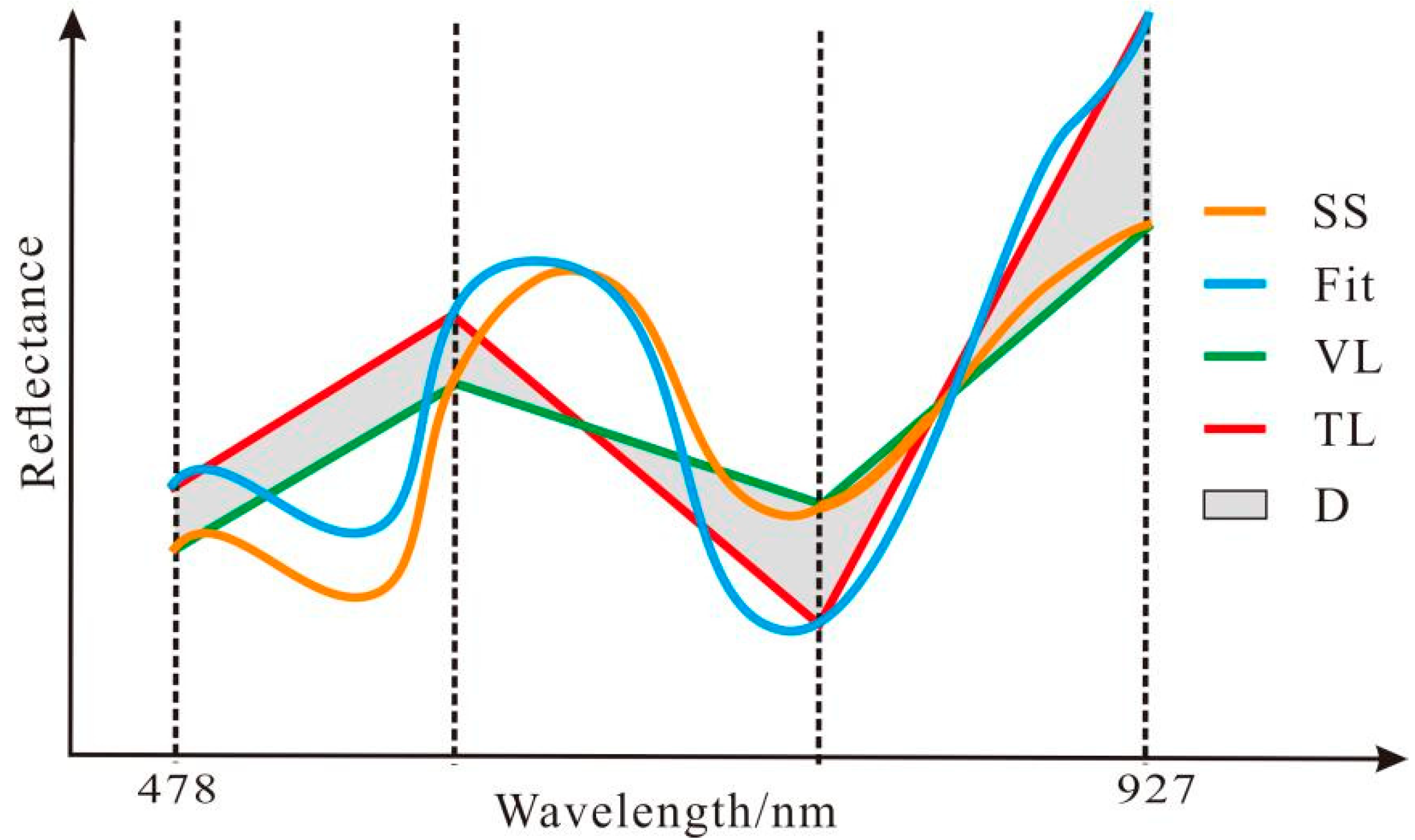
2.3.1. The Simulated Spectrum Method

Multispectral satellites have obvious advantages in earth observation at regional and global scales. However, they have fewer spectral details to reflect the trait information of grassland compared with the hyperspectrum, which limits the prediction accuracy of biomass [40]. The hyperspectrum of the pure endmembers of green grass was acquired on the ground scale. This involved 751 bands in the visible near-infrared (325–1075 nm) range, and could more accurately reflect the grassland details than the multispectrum. If the hyperspectral advantage of the ground-scale is combined with the spatial advantage of multispectral satellites, the biomass estimation accuracy can be effectively improved on a large-scale.
Based on this, this research attempted to obtain the hyperspectrum of the pure endmembers at the main surface objects. According to the principle of mixed pixel decomposition, the fitted spectrum of the multispectral satellite is reversely derived from the pure endmembers and the abundance weight of the ground features. This study area is mainly natural grassland in the growing season, and the proportion of green grass is relatively high. It can be assumed that the main endmember types on the ground are bare soil and green grass. Additionally, the fitted spectrum can be calculated as follows:
F i t λ = j = 1 n f j × p λ , j  
where   λ   is   the   wavelength ,     F i t λ is the fitted hyperspectral according to the abundance of ground objects, f j is the weight of the class j in unit pixels, and p λ , j is the reflectivity of the class j pure pixel at λ. For large-scale grassland, it can be assumed that the mixed spectrum of Sentinel-2 unit pixels is only affected by grass and bare soil, and the vegetation coverage can be calculated by the following Formula (2) [41]:
{ f v = N D V I V s o i l V v e g V s o i l × 100 % f s = 1 f v                                            
where f v is the vegetation coverage (%); f s is the proportion of bare soil in the unit pixels (%); NDVI is the normalized vegetation index calculated by multispectral satellite imagery; and V v e g and V s o i l are NDVI values calculated under pure pixels of grass and bare soil, respectively. In this article, these pure endmembers are observed spectra by ASD spectrometer. Moreover, the hyperspectral images (e.g., EO-1 Hyperion) can also be used to obtain pure endmember spectrum in unknown areas. In Formula (2), the V v e g and V s o i l are used as threshold values of vegetation and soil, respectively, to calculate the vegetation coverage of the entire area.
NDVI is a vegetation index based on the spectral characteristics of vegetation with high reflection in the near-infrared band and strong absorption in the red light band. It has a high sensitivity to vegetation changes and can effectively distinguish vegetation from soil [42]. Its calculation formula is as follows:
N D V I = R n i r R r e d R n i r + R r e d
where R n i r and R r e d are the reflectivity of multispectral satellites in near-infrared and red light bands, respectively.
Then, the Fit can be optimized by the multispectral satellite. The reason for this is that the Fit is fitted by the hyperspectral endmembers and their abundance weight, and its essence is point data reflecting the characteristics of endmembers. However, for the Sentinel-2 image pixel (10 × 10 m2), its reflection characteristics are determined by the ground objects and environment within 100 m2, such as texture characteristics, the ground object abundance, topographic undulations, vegetation types, etc., and its essence is a synthesis of area data. Therefore, using the multispectral satellite to calibrate Fit can reflect the overall characteristics of the pixel scale and increase the spectral detail information of the main feature endmembers. The simulated spectral process is shown in Formulas (4)–(7).
S S λ = D λ + F i t λ
Here, S S λ is the simulated spectrum at λ , there are 751 bands, and the hyperspectral detail is added based on the raw multispectrum, and D λ is the correction coefficient at λ , which is used to solve the inconsistency between the reflectivity trend of SS and true spectral information of Sentinel-2. The correction coefficient can be calculated by Formula (5).
D λ = V L λ T L λ
Here, V L λ is the vector line of multispectral satellite reflectance, which could be considered a continuous piecewise function of remote sensing satellite (Sentinel-2) reflectivity, and T L λ is the trend line of F i t λ , which was segmented by the central wavelength of a multispectral satellite.
T L λ = { a 1 λ + b 1 ,               W 1 λ < W 2 a 2 λ + b 2 ,               W 2 X < W 3 a k 1 λ + b k 1 ,   W k 1 λ W k
Here, W k is the central wavelength of the k-th band of the multispectral (k ≥ 2), a k and b k are the slope and intercept of TL in the interval [ W k 1 , W k ] , respectively, and the calculation formula is as follows:
{ a k 1 = F i t W k F i t W k 1 W k W k 1 b k 1 = F i t W k 1 a k 1 W k 1
where F i t W k   is the value of F i t at the central wavelength W k , and F i t W k   F i t .
The satellite reflectivity better reflects the spectral information of the canopy on a large-scale, and the main purpose of this study was to increase the spectral details of the multispectrum by the simulated spectrum method. As shown in Figure 2, it was assumed that V L is the raw reflectance obtained by the satellite and F i t is the spectral curve fitted according to the weight of the ground objects. The Fit was divided based on the center wavelength of the multispectrum, and the TL was formed by connecting the first and last points of each interval. D ( D = V L T L ) represents the distance between the trend line and the satellite reflectivity. When D > 0, T L is too low; when D < 0, T L is too high; and when D = 0, TL is close to V L . The Fit was modified based on distance D, and the SS was finally obtained.

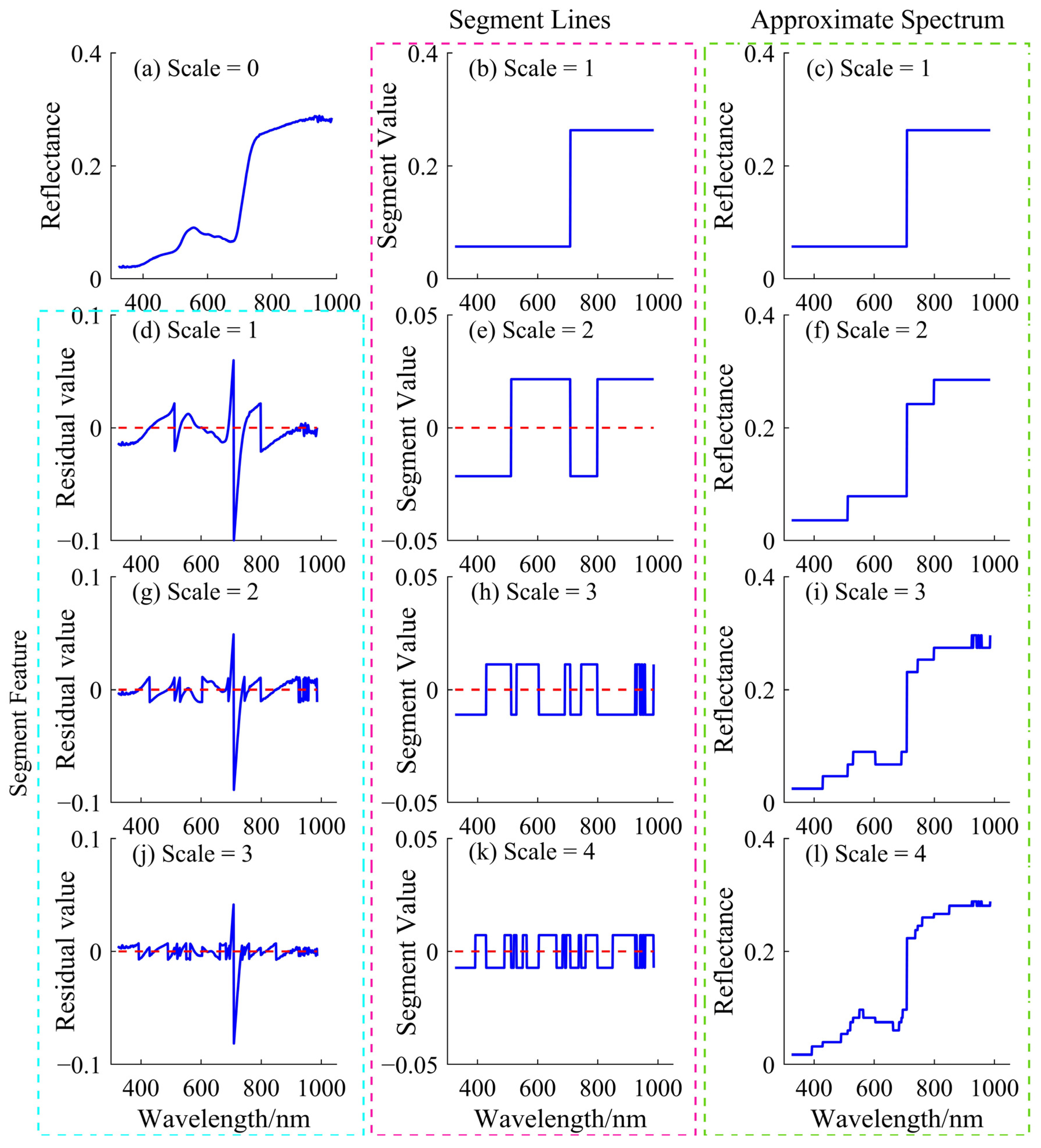
2.3.2. Spectral Segmentation Features

The multi-granularity spectral segmentation method [43] is a new spectral feature extraction technique that was deduced by Kang et al., based on the spectral high-order binary coding (HOBC) method. HOBC is an encoding method that realizes data compression and restoration by transforming the data storage format, such as transforming 16-bit data into 12-bit data. Many details will be lost in the conversion process. These easily lost spectral details may be more sensitive to biomass. Based on this, this method of data segmentation is used to extract spectral information, and its essence is a continuous operation of de-averaging the spectrum to highlight the weak spectrum information within a certain wavelength range. It is assumed that the spectral vector can be approximated by the sum of the products of the M (M > 0)-order segment value and its coefficients, and the residual error decreases with the increase of M:
V = i = 1 M β i H i + R M ( V ) i = 1 M β i H i
where Hi is the ith order segment value of the spectral vector V, H i { 1 , 1 } M ; βi is the coefficient of Hi, βi > 0; and RM(V) is the residual vector of the M-order quantized estimation of V. Through convex optimization, the analytical solution of Formula (8) is [44]
{ β i = 1 N R i 1 ( V ) L 1 H i = sign ( R i 1 ( V ) )
where i = 1, 2, …, M; N is the number of spectral bands; L1 represents 1-norm; and sign() is a sign function, where, when T ≥ 0, sign(T) = 1, and when t < 0, sign(T) = −1.
According to Formulas (8) and (9), the spectral segmentation process can be summarized as the following formula:
{ S F i = S F i 1 S L i S L i = β i × H i A S i = t = 1 i S L t
where S F i is the segmentation feature (SF) after the i-th spectral segmentation, which also includes the features used to construct the biomass estimation model in this article. S L i is the segment line for dividing SF at the i-th spectral segmentation. A S i is the approximate spectrum after i-th spectrum segmentation, and its essence is to gradually approach the original hyperspectral by continuously accumulating from the segment values. The AS is mainly used for data compression of the hyperspectral. Different from AS, the essence of SF is to continuously de-average the original hyperspectral to highlight the detailed information in the spectrum, which helps to improve the estimation accuracy of biomass.
A vegetation spectrum is taken as an example to illustrate the multi-granularity spectral segmentation algorithm (MGSS) (Figure 3), and the part about the segmentation features is explained. Figure 3a presents a typical vegetation hyperspectral curve, its segmentation lines are regarded as itself, and the approximate spectral vector is 0. Figure 3b shows the segment line ( S L 1 = β 1 × H 1 ) of the first segmentation. Then, the first segmentation feature ( S F 1 = S F 0 S L 1 ) was calculated (Figure 3d), and Figure 3c displays the approximate spectrum of the original spectrum after one segmentation. Next, β 2 and H 2 were calculated according to Formula (9), and the second segmentation baseline ( S L 2 = β 2 × H 2 ) was calculated according to Formula (10), after which the second segmentation feature (SF2) was extracted. SF1–SF30 were extracted by repeating the above process.
In this study, the MGSS method was used to extract the spectral segmentation features of the raw spectrum and the simulated spectrum at different scales. These features have good effects on the biomass and element content.

2.3.3. Selection of Vegetation Indices

The vegetation indices (VIs) are correlated with AGB, and according to previous studies and relevant references, a total of 19 VIs were used to estimate AGB (Table 1). The RS-VIs were calculated based on the raw spectrum (RS) of Sentinel-2 and SS-VIs were calculated based on SS.

2.3.4. Above-Ground Biomass Estimation and the Accuracy Evaluation Index

The flowchart in Figure 4 illustrates the experimental methodology used in the study, including the data, method, results, and evaluation. The data mainly include the measured AGB and endmember spectrum data. The simulated spectrum method was proposed to increase the amount of information in the multispectrum, and different spectral features of RS-SF, SS-SF, RS-VIs, and SS-VIs were extracted from RS and SS. Then, those features were used to estimate grassland AGB by PLSR and MSR models.
To evaluate the applicability of the simulated spectrum method to improve the ability of the multispectral satellite to predict grassland AGB, the coefficients of determination (R2), the prediction accuracy (EA), the ratio of performance to deviation (RPD), and the root mean square error (RMSE) and its bias-standard deviation decomposition [59,60] were used.

3. Results

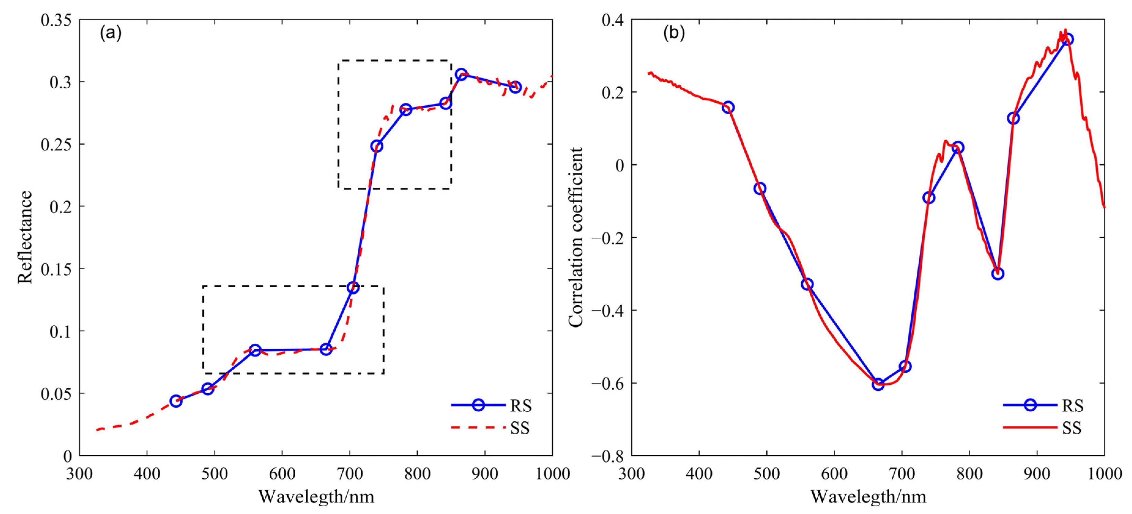
3.1. Satellite-Scale Simulated Spectrum

As shown in Figure 5a, the blue and red lines represent the RS and SS at wavelengths of 375–1000 nm, respectively. The RS is the overall response within the range of the unit pixels (10 × 10 m2), and its reflectivity is closely related to the surface environment, such as vegetation coverage, soil moisture, etc., so the SS does not change the reflectance of the multispectrum at the center wavelength, and the spectral details of the SS are supplemented based on the surface object type and its abundance. Compared with RS, SS has two advantages: (i) The SS contains more spectral information from endmembers, as shown in the black dashed box in Figure 5a, and (ii) due to the design of the sensor, Sentinel-2 did not collect data with a wavelength in the range of 375–445 nm, the pure endmembers obtained by ASD have continuous reflection information in this range, and the data of Sentinel-2 are supplemented by the spectral simulation algorithm in the range of 375–445 nm. All these reflection features may contain useful information for biomass estimation. Moreover, the correlation between biomass and SS and RS was analyzed, respectively, and the results showed that the correlation of SS is better than RS in some frequency bands (Figure 5b). For example, in the wavelength range of 560–665 nm, the R of SS is closer to −1 than RS, which is better than band 3, and in the range of 865–945 nm, SS and RS are positively correlated with biomass, and the R of SS is higher than that of RS, which also means that SS has more advantages when using different band combinations to estimate biomass. Therefore, the simulated spectrum method can increase the sensitivity information of Sentinel-2 to biomass.

3.2. Correlation Analysis of Biomass and the Vegetation Index

RS-VIs and SS-VIs were calculated by RS and SS to test the effectiveness of the simulated spectrum methods, and the correlation between the two vegetation indices and AGB were compared and analyzed. The results are shown in Figure 6. Except for the TSAVI and GNDVI, other indexes have a good correlation with AGB (R > 0.6), so the vegetation index is a relatively concise method for estimating biomass. Additionally, the correlation of SS-VIs is better than that of RS-VIs, which is more suitable for AGB estimation. Among the 19 vegetation indices, the correlation coefficients of RS-VIs and SS-VIs are equivalent in RVI and RDVI, and those of RS-VIs are slightly higher than those of SS-VIs in NDVI705 and MSAVI. However, SS-VIs are better than RS-VIs in other indexes, with MTCI, DVI, EVI, and SAVI increasing by more than 0.1 in R. This is because SS has more spectral information related to the surface, and can select suitable bands within a sensitive range to construct a narrow-band vegetation index. Therefore, the simulated method can increase the selectivity of spectral features and improve the estimation ability of multispectral satellites when estimating biomass with a single vegetation index.

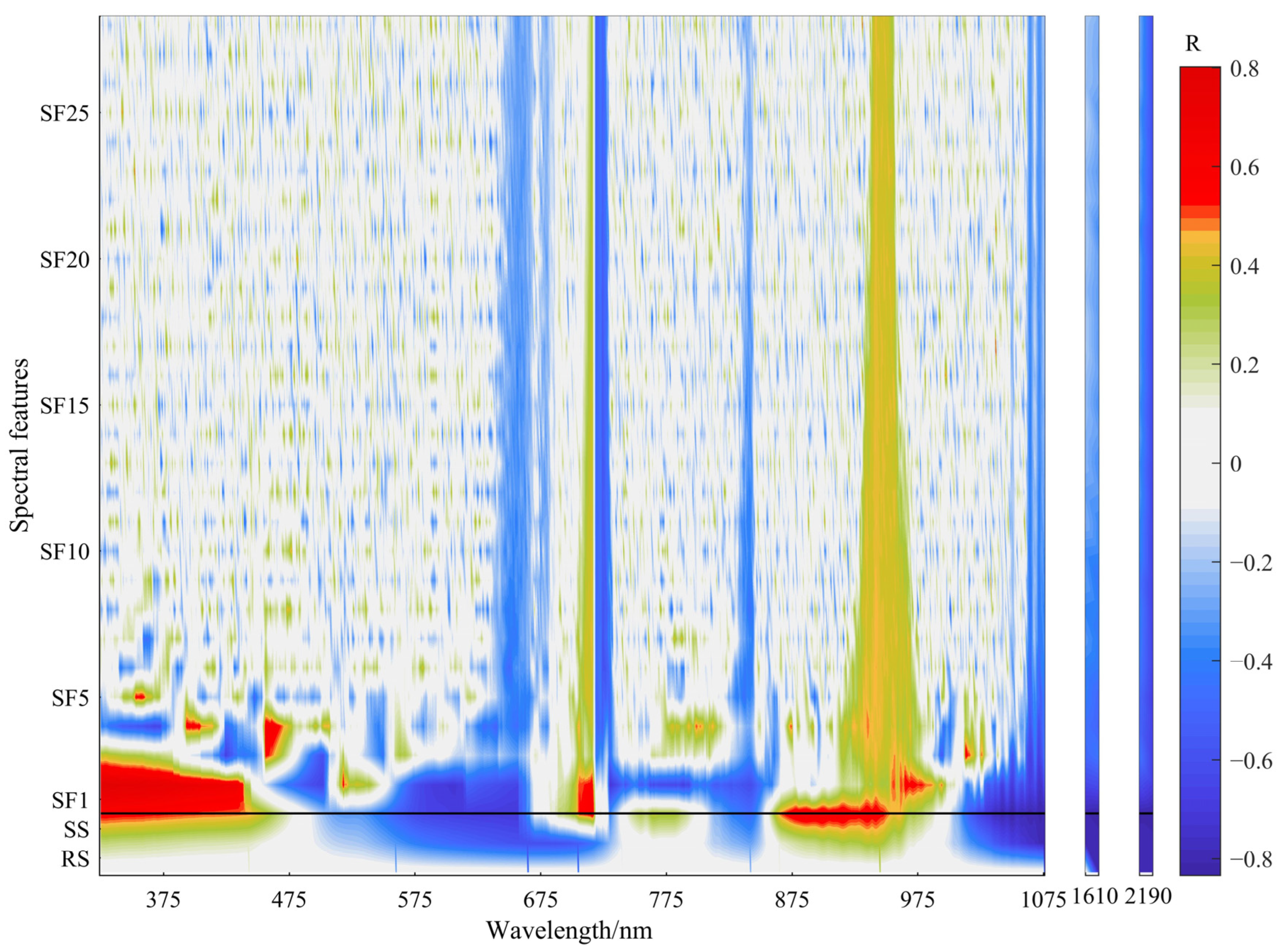
3.3. Segmentation Feature Extraction of the Spectrum

The SS enhances the spectral information of multispectral satellites by the simulated spectrum method, but it also has certain drawbacks. On the one hand, due to the addition of a large number of spectral details after being simulated, the difficulty of image storage and processing is increased; on the other hand, SS has certain data redundancy, which restricts the estimation accuracy of biomass.
The MGSS method has become an effective means to solve those problems. As shown in Figure 7, RS represents the raw spectrum of Sentinel-2, which contains 12 bands, and there are only two bands that have correlation coefficients with absolute values above 0.6. Moreover, the best R is –0.79; SS represents the stimulated spectrum, which contains 731 band features, and has 61 bands with | R | |R| above 0.6, and there are four high correlation intervals at 575–703, 1025–1075, 1610, and 2190 nm. Therefore, RS has fewer spectral features than SS. However, the reflection characteristics between SS bands are extremely similar, and the redundancy reduces the data quality: the one-dimensional SS is divided into 30 features (SF1–SF30) through the MGSS method. In RS and SS, the spectrum and AGB are mainly negatively correlated, but correlations have a mixed distribution of positive and negative on SF1–SF30, which is conducive to reducing data redundancy and improving the spectral sensitivity. As the segmentation scale increases, the difference between adjacent bands gradually increases. As shown, the wavelength range with a similar correlation gradually shatters and shrinks, and finally, three highly correlated narrow bands of 705–725, 925–975, and 2190 nm are formed, which become sensitive bands related to biomass.
The sequence forward selection (SFS) method can not only select the bands with a higher correlation with biomass, but also take into account the combined effect between the selected features. The sensitive bands were selected by SFS for RS, SS, and SF1–SF30, and those bands exhibited a high correlation with biomass and low correlation among each band. As shown in Figure 8, the horizontal axis is the wavelength, the vertical axis is the spectral feature type, the circles represent the selected sensitive bands, and the different colors indicate the priority order of band selection at a single scale. Among the 12 raw bands of RS, only eight bands meet the requirements after SFS selection, which are mainly concentrated near the red edge (675–875 nm). Compared with RS, SS has 16 sensitive bands to be selected, among which four visible light bands are supplemented and six bands are supplemented in near-infrared and shortwave infrared ranges. SF1–SF30 can have more than 16 bands to meet the standard, and these bands are discretely distributed between 375 and 2190 nm, indicating that the MGSS method can reduce the redundancy and mine the weak spectral information related to biomass. Through the MGSS algorithm, the redundancy between the SS bands can be reduced. Through the SFS band selection method, the sensitive bands related to biomass are selected and stored, which effectively reduces the amount of SS data.

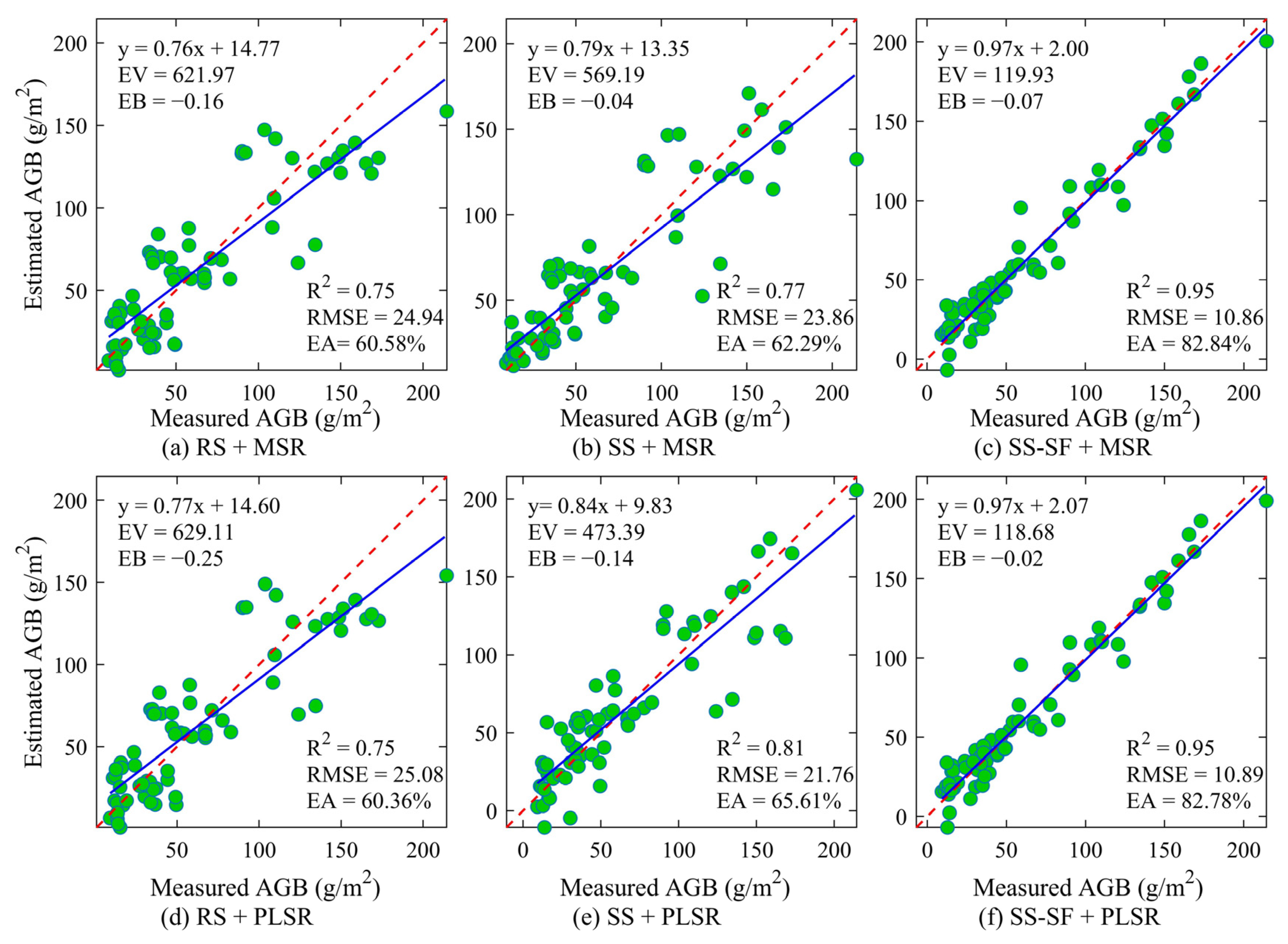
3.4. Biomass Estimation Model and Accuracy Evaluation

The accuracy of biomass prediction is the basis for determining whether the simulated spectrum method can effectively improve the utilization rate of Sentinal-2. In this paper, SS, RS, SS-VIs, and RS_VIs were used to construct MSR and PLSR biomass estimation models, and a 10-fold cross-validation approach was used to verify the accuracy. To avoid modeling errors caused by unreasonable sample partitioning, all of the AGB data were sorted into a descending sequence and divided into 10 equal parts. One-tenth of the data were used for verification, and the remaining points were used to build the model. After 10 cycles of this, the estimation accuracy was as shown in Table 2. The biomass estimation results of SS were better than those of RS. Compared with RS, the coefficient of determination (R2) of SS increased from 0.77 to 0.75 in the MSR model, and 0.75 to 0.81 in the PLSR model. The accuracy of SS in the three evaluation indicators of RMSE, EA, and RPD was also improved; under the characteristics of the vegetation index, SS-VI is better than RS-VI when a single vegetation index is used to estimate biomass, and the highest R2 of SS-VI is 0.70. However, the accuracy of SS-VI is lower than that of RS-VI when multiple vegetation indices are used as parameters for estimating biomass. It may be that when sensitive bands were selected to construct the SS-VI, it focused more on the correlation between a single vegetation index and biomass, while ignoring the collinearity between vegetation indexes. Therefore, SS-VI is better than RS-VI in a single index model, and RS-VI is better than SS-VI in a multiple vegetation index model. There may be two factors that limit the advantages of SS. On the one hand, the VIs are simple to calculate, and only two-three dominant bands are used, which cannot fully utilize the advantages of the hyperspectral; on the other hand, there is collinearity among the VIs. In the segmentation features, affected by the amount of spectral information, the RS-SF estimation accuracy is poor. However, SS-SF fully utilizes the spectral advantages of SS, and the estimation accuracy is better than that of RS, SS, RS-VIs, and SS-VIs. In the MSR and PLSR estimation models, R2 reaches 0.95, RMSE is less than 11 g/m2, EA is greater than 82.5%, and RPD is above 4.6, which shows that the model has a high stability.
The relationship between the measured and estimated AGB using RS, SS, SS-SF, and MSR and PLSR is shown in Figure 9. The results indicate that the estimation accuracy of RS is the lowest, the error is large (RMSE = 24.94–25.08 g/m2), the scattered points are distributed on both sides of the 1:1 straight line, and EA < 60.60%; (ii) compared with RS, the accuracy of SS inversion is improved, RMSE is reduced by 1.08–3.32 g/m2, and EA is increased by 1.71–5.25%. The accuracy of the SS model is higher in low biomass regions, but the error is still large in high biomass regions; and (iii) SS-SF provides a better estimation accuracy in MSR and PLSR models: R2 > 0.95; EA > 82.84%; RMSE reduced by 14.08–14.19 g/m2 in comparison to RS; and the scattered points are concentrated on the 1:1 line. The inclination amplitude of the SS-SF fitting line and the 1:1 line indicates that the model estimation is more accurate in the medium and low biomass environment, and it is easily underestimated in the high biomass environment. This may be because there are fewer sampling points in the high biomass area. In the RS and SS models, AGB is easily overestimated in low biomass areas and underestimated in high biomass areas, which also causes the error variance and the error bias to be generally greater than SS-SF models. In the comparison of the model accuracy, the MSR and PLSR models have similar results, indicating that the simulated spectrum and the spectral segmentation method can improve the accuracy of large-scale biomass estimation in Sentinel-2 images.

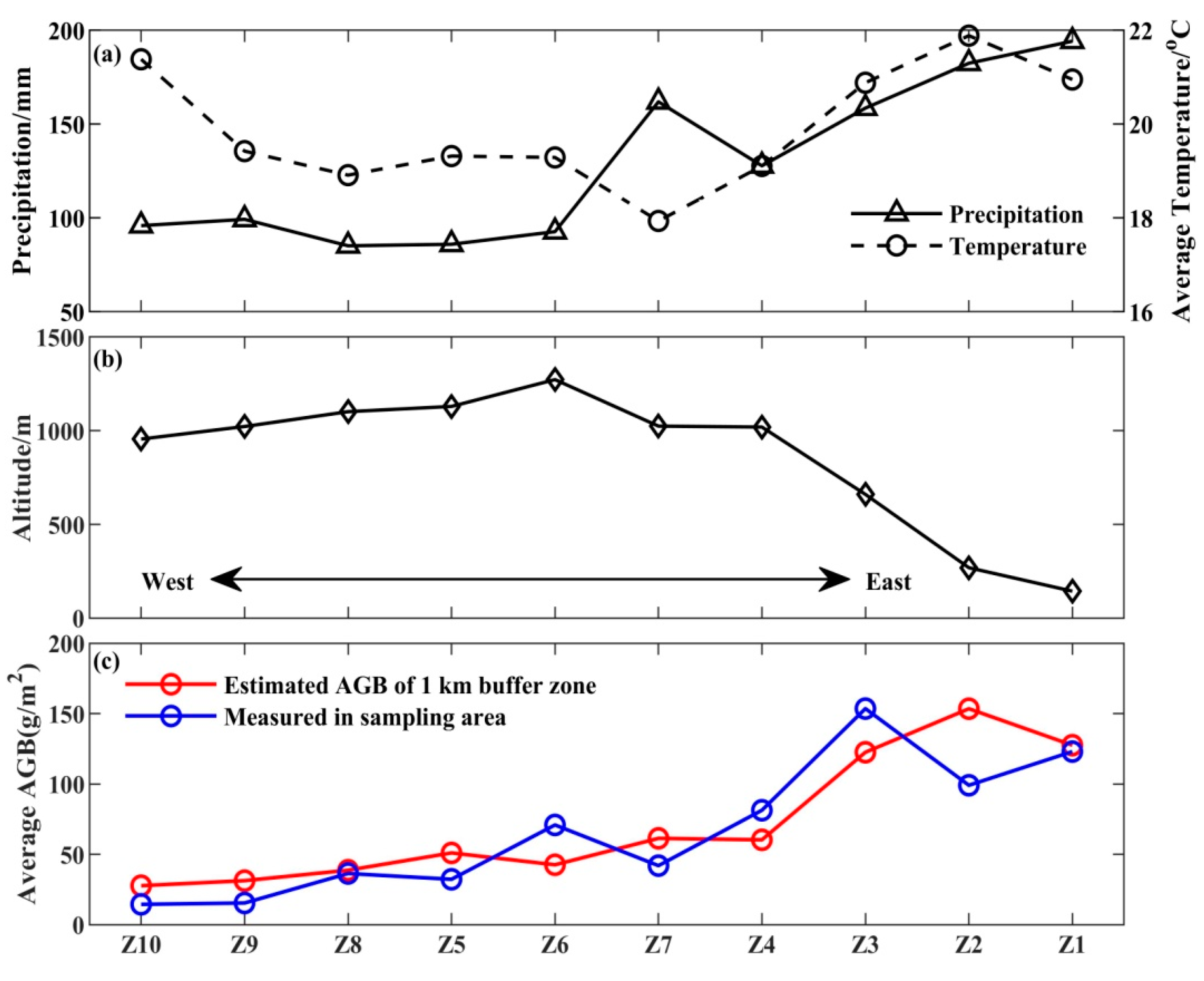
3.5. Spatial Variation of Biomass in Longitude

In this study, MSR and PLSR had an approximate estimation accuracy based on the validation set and taking into account the computational difficulty of the two models, the SS-SF+MSR model was used to construct an AGB estimation model. At the same time, to verify the ability to estimate AGB by the simulated spectrum system on a large-scale, in each sampling area (S1–S10), the AGB within a 1 km radius circle (Z1–Z10) was estimated and mapped. The original image (RGB true color synthesis) and biomass distribution are shown in Figure 10. The color from green to red represents the biomass from low to high, and the white hollow area in the figure is a thick cloud or road (masked). It can be seen that the spatial distribution of biomass content has a high degree of agreement with the location of green vegetation. Taking Z2 as an example, the green vegetation distribution area in the true-color image has a higher biomass (>150 g/m2), and the areas such as shadows and roads have a low biomass (<60 g/m2), which is significantly different from vegetation. It can be qualitatively concluded that the estimated biomass has a certain accuracy.
Furthermore, the reliability of estimation based on the spatial location and climatic conditions of Z1–Z10 was analyzed and evaluated. Figure 11a shows the average temperature and precipitation in the sampling area from the period of grass turning green to the sampling cut-off period (1 May to 14 July), Figure 11b shows the altitudes of Z1–Z10, and Figure 11c shows the measured AGB in the sampling area and the estimated AGB in the 1 km buffer zone. The latitudes of Z1–Z10 are similar, with obvious longitude changes from east to west, and the climate characteristics transition from those of a monsoon climate to those of a continental climate. Therefore, in theory, grassland biomass will gradually decrease, and the estimation of AGB on the satellite-scale is consistent with the theory. Z1, Z2, and Z3 are located in warm and humid plains and hilly areas, with an altitude of <660 m, an average temperature of >20 °C, precipitation of >150 mm, and high biomass (>120 g/m2); Z4–Z10 forage grass has poor growth conditions and is located in the Inner Mongolia Plateau, with an altitude of >950 m, the temperature is between 18 and 22 °C, there is little precipitation, and the biomass is generally below 40 g/m2.
Although there is a certain gap between the measured average value of biomass in the sampling area (S1–S10) and the estimated value in the buffer zone (Z1–Z10), it must be highlighted that S1–S10 are only the eight samples within each 1 × 1 m2. For the average value of biomass, the selection of plots is random and localized, while Z1–Z10 is the AGB within 1 km of each plot of S1–S10, and the estimation results are more global. Among them, S2 and Z2, S3 and Z3, and S6 and Z6 are quite different. The main reason for this is that the influence of thin clouds in these areas is more serious than in other sample areas, which restricts the estimation accuracy. In summary, the SS-SF + MSR model can accurately estimate biomass information on a large scale.

4. Discussion

4.1. Biomass Estimation Model Based on the Simulated Spectrum

Multispectral satellites have the advantages of a large width, low cost, and high-efficiency in-ground monitoring, and are still the main means of large-scale grassland character monitoring [21]. However, their low spectral resolution has become the key point that restricts the accuracy of multispectral satellite inversion of grassland characteristics. In the past, satellite image selection was often aimed at pursuing efficiency or precision. For efficiency, the inversion error caused by the lowspectral resolution of multispectral images is always ignored. For the inversion accuracy, selecting hyperspectral imagery as the data source does improve the estimation accuracy [61]. However, hyperspectral satellite images are expensive, with scarce data and a narrow width [62], so are difficult to apply in a wide range. Additionally, many scholars focus on studying the scale effect of remote sensing images to improve the inversion accuracy of low-resolution satellites [63]. In satellite scale conversion, scaling up is easy to operate, but scaling down is still an unsolved hot spot in remote sensing [64].
Compared with the multispectrum, the higher inversion accuracy of the simulated spectrum is due to the fact that it has more spectral details, which can distinguish the ground objects from the different wavelengths. The same species has approximate spectral characteristics, so we can fit the pure pixel spectral detail features to the satellite-scale multispectrum according to the grassland vegetation type and its vegetation coverage, so that multispectral satellites can have more detailed spectral information and improve the earth-monitoring ability of multispectral satellites. The experiment in this paper preliminarily proves that this spectral derivation method can feasibly improve the precision of satellite image inversion.
The vegetation index is a key parameter for many vegetation character estimation models [13,65], and limits the estimation accuracy of AGB. VIs calculated using wide-band multispectral satellites will be supersaturated in high vegetation coverage areas [33]. The simulated spectrum algorithm can enrich the spectral information of multispectral images so that sensitive bands can be selected according to the characteristics of plants in the pseudo-hyperspectral range, and the optimal spectral index can be constructed, which can improve the prediction accuracy of key characters such as biomass.
The experiment in this paper preliminarily proves that this simulated spectrum method has certain feasibility for improving the accuracy of satellite image inversion. Compared with RS directly used for biomass estimation, the estimation accuracy of SS-SF for biomass is improved by 7–17%. Compared with Sentinel-2, the derivative transformation method may be more effective if this method is used in Landsat which has little information, and the next step will be an in-depth study to investigate this.

4.2. Uncertainties and Sources of Error

There are certain difficulties and uncertainties in the large-scale inversion of grassland traits based on remote sensing. The grassland ecosystem itself is complex and the grass species type, growth height, and growth stages (greening, heading, flowering, maturing, and yellowing) all lead to differences in grassland characteristics [66]. Moreover, the topography, climatic environment, nutrient content (N and P), water stress, etc. can also affect the spectral reflectivity of grasses, so the construction and applicability of the biomass inversion model are challenging.
The error of the data also affects the prediction accuracy, mainly including field measurement error and image error. In the process of measuring biomass on the ground, instrument errors and operational errors are inevitable, and are relatively small. There is uncertainty in the scale correspondence between the spatial resolution of the remote sensing image and field measurement [67], but it is difficult to obtain field measurement data corresponding to Landsat (30 m) or Sentinel-2 (10 m) pixels in a large scale range: clouds have always been the key to constraining image quality, especially for satellites with a low time resolution (Landsat, etc.). It is easy to have a vacuum of data during the growth stage of grassland, which is out of step with the time of field measurement data, thus increasing the difficulty of grassland biomass inversion.
In the process of large-scale grassland character prediction, those uncertainties and data errors are inevitable. In this study, the spectral derivative method was selected to improve the precision of satellite-scale biomass inversion. In future research, the spatial scale factor will be introduced into the spectral derivation process to explore the precision of grassland biomass inversion in different growth stages.

5. Conclusions

Using Sentinel-2 imagery as the data source, this paper proposes a biomass estimation method under the satellite-scale simulated spectrum system. This method was used to estimate the grassland biomass in the 44°N latitude zone of the Inner Mongolia Plateau, and the estimation accuracy was evaluated qualitatively and quantitatively. The main conclusions are as follows.
To improve the spectral resolution of multispectral satellite images, a simulated spectral method is proposed, which combines the advantages of endmember hyperspectral information and Sentinel-2 space to construct a satellite-scale pseudo-hyperspectral image (SS-Sentinel). Compared with RS, SS has more spectral details, and the correlation between reflection features of some bands and biomass is better than that of RS, and the SS-VIs based on SS are better than RS-VIs.
Based on SS, the segmentation feature SS-SF, which was extracted by the MGSS method, was employed to construct MSR and PLSR AGB estimation models, and the estimation accuracy of AGB was greatly improved. The AGB was estimated by RS features, resulting in R2 = 0.75 and RMSE = 24.94–25.08 g/m2 upon verification. Compared with RS, the R2 of SS-SF increased by 0.2, RMSE decreased by 14.08–14.19 g/m2, and EA increased by 22.26–22.42%.
Therefore, the simulated spectrum method can improve the inversion accuracy of grassland biomass by multispectral satellites, and provide a new idea for the accurate inversion of regional and global large-scale biomass.

Author Contributions

Conceptualization, H.P. and A.Z.; methodology, H.P.; validation, H.P.; formal analysis, H.P.; investigation, H.P., X.K., G.D. and N.H.; resources, A.Z., G.D. and N.H.; writing—original draft preparation, H.P.; writing—review and editing, H.P., A.Z. and X.K.; supervision, A.Z.; project administration, A.Z. and N.H. All authors have read and agreed to the published version of the manuscript.

Funding

This research was funded by the National Natural Science Foundation of China, Grant Number 42071303, and Special Foundation for Science and Technology Basic Resource Investigation Program of China, Grant Number 2019FY101304.

Acknowledgments

The authors thank Kong of Ludong University for his valuable guidance and suggestions.

Conflicts of Interest

The authors declare no conflict of interest.

References

  1. Ramoelo, A.; Cho, M.A.; Mathieu, R.; Madonsela, S.; Van De Kerchove, R.; Kaszta, Z.; Wolff, E. Monitoring grass nutrients and biomass as indicators of rangeland quality and quantity using random forest modelling and WorldView-2 data. Int. J. Appl. Earth Obs. Geoinf. 2015, 43, 43–54. [Google Scholar] [CrossRef]
  2. Schino, G.; Borfecchia, F.; De Cecco, L.; Dibari, C.; Iannetta, M.; Martini, S.; Pedrotti, F. Satellite estimate of grass biomass in a mountainous range in central Italy. Agrofor. Syst. 2003, 59, 157–162. [Google Scholar] [CrossRef]
  3. Houghton, R.A.; Hall, F.; Goetz, S.J. Importance of biomass in the global carbon cycle. J. Geophys. Res. Biogeosciences 2009, 114. [Google Scholar] [CrossRef]
  4. Lu, D. The potential and challenge of remote sensing-based biomass estimation. Int. J. Remote Sens. 2006, 27, 1297–1328. [Google Scholar] [CrossRef]
  5. Kumar, L.; Sinha, P.; Taylor, S.; Alqurashi, A.F. Review of the use of remote sensing for biomass estimation to support renewable energy generation. J. Appl. Remote Sens. 2015, 9, 097696. [Google Scholar] [CrossRef]
  6. Knipling, E.B. Physical and physiological basis for the reflectance of visible and near-infrared radiation from vegetation. Remote Sens. Environ. 1970, 1, 155–159. [Google Scholar] [CrossRef]
  7. Houborg, R.; McCabe, M.F.; Cescatti, A.; Gitelson, A.A. Leaf chlorophyll constraint on model simulated gross primary productivity in agricultural systems. Int. J. Appl. Earth Obs. Geoinf. 2015, 43, 160–176. [Google Scholar] [CrossRef] [Green Version]
  8. Yue, J.; Yang, G.; Tian, Q.; Feng, H.; Xu, K.; Zhou, C. Estimate of winter-wheat above-ground biomass based on UAV ultrahigh-ground-resolution image textures and vegetation indices. ISPRS J. Photogramm. Remote Sens. 2019, 150, 226–244. [Google Scholar] [CrossRef]
  9. Féret, J.-B.; Gitelson, A.A.; Noble, S.D.; Jacquemoud, S. PROSPECT-D: Towards modeling leaf optical properties through a complete lifecycle. Remote Sens. Environ. 2017, 193, 204–215. [Google Scholar] [CrossRef] [Green Version]
  10. Labus, M.P.; Nielsen, G.A.; Lawrence, R.L.; Engel, R.; Long, D.S. Wheat yield estimates using multi-temporal NDVI satellite imagery. Int. J. Remote Sens. 2002, 23, 4169–4180. [Google Scholar] [CrossRef]
  11. Fu, Y.; Yang, G.; Wang, J.; Song, X.; Feng, H. Winter wheat biomass estimation based on spectral indices, band depth analysis and partial least squares regression using hyperspectral measurements. Comput. Electron. Agric. 2014, 100, 51–59. [Google Scholar] [CrossRef]
  12. Gnyp, M.L.; Miao, Y.; Yuan, F.; Ustin, S.L.; Yu, K.; Yao, Y.; Huang, S.; Bareth, G. Hyperspectral canopy sensing of paddy rice aboveground biomass at different growth stages. Field Crops Res. 2014, 155, 42–55. [Google Scholar] [CrossRef]
  13. Cabrera-Bosquet, L.; Molero, G.; Stellacci, A.; Bort, J.; Nogués, S.; Araus, J.L. NDVI as a potential tool for predicting biomass, plant nitrogen content and growth in wheat genotypes subjected to different water and nitrogen conditions. Cereal Res. Commun. 2011, 39, 147–159. [Google Scholar] [CrossRef]
  14. Wang, L.; Zhou, X.; Zhu, X.; Dong, Z.; Guo, W. Estimation of biomass in wheat using random forest regression algorithm and remote sensing data. Crop J. 2016, 4, 212–219. [Google Scholar] [CrossRef] [Green Version]
  15. Jay, S.; Baret, F.; Dutartre, D.; Malatesta, G.; Héno, S.; Comar, A.; Weiss, M.; Maupas, F. Exploiting the centimeter resolution of UAV multispectral imagery to improve remote-sensing estimates of canopy structure and biochemistry in sugar beet crops. Remote Sens. Environ. 2019, 231, 110898. [Google Scholar] [CrossRef]
  16. Han, L.; Yang, G.; Yang, H.; Xu, B.; Li, Z.; Yang, X. Clustering Field-Based Maize Phenotyping of Plant-Height Growth and Canopy Spectral Dynamics Using a UAV Remote-Sensing Approach. Front. Plant Sci. 2018, 9, 1638. [Google Scholar] [CrossRef] [Green Version]
  17. Kefauver, S.C.; Vicente, R.; Vergara-Díaz, O.; Fernandez-Gallego, J.A.; Kerfal, S.; Lopez, A.; Melichar, J.P.E.; Molins, M.D.S.; Araus, J.L. Comparative UAV and Field Phenotyping to Assess Yield and Nitrogen Use Efficiency in Hybrid and Conventional Barley. Front. Plant Sci. 2017, 8, 1733. [Google Scholar] [CrossRef]
  18. Yu, N.; Li, L.; Schmitz, N.; Tian, L.F.; Greenberg, J.A.; Diers, B.W. Development of methods to improve soybean yield estimation and predict plant maturity with an unmanned aerial vehicle based platform. Remote Sens. Environ. 2016, 187, 91–101. [Google Scholar] [CrossRef]
  19. Holman, F.H.; Riche, A.B.; Michalski, A.; Castle, M.; Wooster, M.J.; Hawkesford, M.J. High Throughput Field Phenotyping of Wheat Plant Height and Growth Rate in Field Plot Trials Using UAV Based Remote Sensing. Remote Sens. 2016, 8, 1031. [Google Scholar] [CrossRef]
  20. Hu, P.; Chapman, S.C.; Wang, X.; Potgieter, A.; Duan, T.; Jordan, D.; Guo, Y.; Zheng, B. Estimation of plant height using a high throughput phenotyping platform based on unmanned aerial vehicle and self-calibration: Example for sorghum breeding. Eur. J. Agron. 2018, 95, 24–32. [Google Scholar] [CrossRef]
  21. Buck, O.; Millán, V.E.G.; Klink, A.; Pakzad, K. Using information layers for mapping grassland habitat distribution at local to regional scales. Int. J. Appl. Earth Obs. Geoinf. 2015, 37, 83–89. [Google Scholar] [CrossRef]
  22. Dube, T.; Mutanga, O. Evaluating the utility of the medium-spatial resolution Landsat 8 multispectral sensor in quantifying aboveground biomass in uMgeni catchment, South Africa. ISPRS J. Photogramm. Remote Sens. 2015, 101, 36–46. [Google Scholar] [CrossRef]
  23. Li, C.; Wulf, H.; Schmid, B.; He, J.-S.; Schaepman, M.E. Estimating Plant Traits of Alpine Grasslands on the Qinghai-Tibetan Plateau Using Remote Sensing. IEEE J. Sel. Top. Appl. Earth Obs. Remote Sens. 2018, 11, 2263–2275. [Google Scholar] [CrossRef]
  24. Immitzer, M.; Vuolo, F.; Atzberger, C. First Experience with Sentinel-2 Data for Crop and Tree Species Classifications in Central Europe. Remote Sens. 2016, 8, 166. [Google Scholar] [CrossRef]
  25. Ustin, S.L.; Gitelson, A.A.; Jacquemoud, S.; Schaepman, M.; Asner, G.P.; Gamon, J.A.; Zarco-Tejada, P. Retrieval of foliar information about plant pigment systems from high resolution spectroscopy. Remote Sens. Environ. 2009, 113, S67–S77. [Google Scholar] [CrossRef] [Green Version]
  26. Schaepman, M.E.; Koetz, B.; Schaepman-Strub, G.; Zimmermann, N.; Itten, K. Quantitative retrieval of biogeophysical characteristics using imaging spectroscopy—A mountain forest case study. Community Ecol. 2004, 5, 93–104. [Google Scholar] [CrossRef]
  27. Vohland, M.; Mader, S.; Dorigo, W. Applying different inversion techniques to retrieve stand variables of summer barley with PROSPECT+SAIL. Int. J. Appl. Earth Obs. Geoinf. 2010, 12, 71–80. [Google Scholar] [CrossRef]
  28. Yue, J.; Yang, G.; Li, C.; Li, Z.; Wang, Y.; Feng, H.; Xu, B. Estimation of Winter Wheat Above-Ground Biomass Using Unmanned Aerial Vehicle-Based Snapshot Hyperspectral Sensor and Crop Height Improved Models. Remote Sens. 2017, 9, 708. [Google Scholar] [CrossRef] [Green Version]
  29. Lu, D.; Batistella, M. Exploring TM image texture and its relationships with biomass estimation in Rondônia, Brazilian Amazon. Acta Amaz. 2005, 35, 249–257. [Google Scholar] [CrossRef]
  30. Kumar, K.K.; Nagai, M.; Witayangkurn, A.; Kritiyutanant, K.; Nakamura, S. Above Ground Biomass Assessment from Combined Optical and SAR Remote Sensing Data in Surat Thani Province, Thailand. J. Geogr. Inf. Syst. 2016, 8, 506–516. [Google Scholar] [CrossRef] [Green Version]
  31. Zheng, H.; Cheng, T.; Zhou, M.; Li, D.; Yao, X.; Tian, Y.; Cao, W.; Zhu, Y. Improved estimation of rice aboveground biomass combining textural and spectral analysis of UAV imagery. Precis. Agric. 2018, 20, 611–629. [Google Scholar] [CrossRef]
  32. Santi, E.; Paloscia, S.; Pettinato, S.; Fontanelli, G.; Mura, M.; Zolli, C.; Maselli, F.; Chiesi, M.; Bottai, L.; Chirici, G. The potential of multifrequency SAR images for estimating forest biomass in Mediterranean areas. Remote Sens. Environ. 2017, 200, 63–73. [Google Scholar] [CrossRef]
  33. Mutanga, O.; Skidmore, A.K. Narrow band vegetation indices overcome the saturation problem in biomass estimation. Int. J. Remote Sens. 2004, 25, 3999–4014. [Google Scholar] [CrossRef]
  34. Cheng, T.; Rivard, B.; Sánchez-Azofeifa, G.A.; Feret, J.-B.; Jacquemoud, S.; Ustin, S.L. Predicting leaf gravimetric water content from foliar reflectance across a range of plant species using continuous wavelet analysis. J. Plant Physiol. 2012, 169, 1134–1142. [Google Scholar] [CrossRef]
  35. Kang, X.; Zhang, A. Hyperspectral remote sensing estimation of pasture crude protein content based on multi-granularity spectral feature. Trans. Chin. Soc. Agric. Eng. 2019, 35, 161–169. [Google Scholar] [CrossRef]
  36. Tian, A.; Zhao, J.; Xiong, H.; Gan, S.; Fu, C. Application of Fractional Differential Calculation in Pretreatment of Saline Soil Hyperspectral Reflectance Data. J. Sen. 2018, 2018, 8017614. [Google Scholar] [CrossRef]
  37. Tang, K.; Wulantuya; Dash, D.; Surina. RS-Based Monitoring of NDVI Spatial Variations: A Case Study of Typical Grasslands on Mongolian Plateau. Nat. Inner Asia 2019, 116, 69–86. [Google Scholar] [CrossRef]
  38. Zhao, Y.; Liu, H.; Zhang, A.; Cui, X.; Zhao, A. Spatiotemporal variations and its influencing factors of grassland net primary productivity in Inner Mongolia, China during the period 2000–2014. J. Arid. Environ. 2019, 165, 106–118. [Google Scholar] [CrossRef]
  39. Gascon, F.; Bouzinac, C.; Thépaut, O.; Jung, M.; Francesconi, B.; Louis, J.; Lonjou, V.; Lafrance, B.; Massera, S.; Gaudel-Vacaresse, A.; et al. Copernicus Sentinel-2A Calibration and Products Validation Status. Remote Sens. 2017, 9, 584. [Google Scholar] [CrossRef] [Green Version]
  40. Capolupo, A.; Kooistra, L.; Berendonk, C.; Boccia, L.; Suomalainen, J. Estimating Plant Traits of Grasslands from UAV-Acquired Hyperspectral Images: A Comparison of Statistical Approaches. ISPRS Int. J. Geoinf. 2015, 4, 2792–2820. [Google Scholar] [CrossRef]
  41. Li, F.; Chen, W.; Zeng, Y.; Zhao, Q.; Wu, B. Improving Estimates of Grassland Fractional Vegetation Cover Based on a Pixel Dichotomy Model: A Case Study in Inner Mongolia, China. Remote Sens. 2014, 6, 4705–4722. [Google Scholar] [CrossRef] [Green Version]
  42. Bhandari, A.K.; Kumar, A.; Singh, G.K. Feature Extraction using Normalized Difference Vegetation Index (NDVI): A Case Study of Jabalpur City. Procedia Technol. 2012, 6, 612–621. [Google Scholar] [CrossRef] [Green Version]
  43. Kang, X.; Zhang, A. A Novel Method for High-Order Residual Quantization-Based Spectral Binary Coding. Spectrosc. Spectr. Anal. 2019, 39, 3013–3020. [Google Scholar]
  44. Li, Z.; Ni, B.; Zhang, W.; Yang, X.; Gao, W. Performance Guaranteed Network Acceleration via High-Order Residual Quantization. In Proceedings of the 2017 IEEE International Conference on Computer Vision (ICCV), Venice, Italy, 22–29 October 2017; pp. 2584–2592. [Google Scholar]
  45. Cho, M.A.; Skidmore, A.; Corsi, F.; Van Wieren, S.E.; Sobhan, I. Estimation of green grass/herb biomass from airborne hyperspectral imagery using spectral indices and partial least squares regression. Int. J. Appl. Earth Obs. Geoinf. 2007, 9, 414–424. [Google Scholar] [CrossRef]
  46. Anderson, G.L.; Hanson, J.D. Evaluating hand-held radiometer derived vegetation indices for estimating above ground biomass. Geocarto Int. 1992, 7, 71–78. [Google Scholar] [CrossRef]
  47. Baret, F.; Guyot, G. Potentials and limits of vegetation indices for LAI and APAR assessment. Remote Sens. Environ. 1991, 35, 161–173. [Google Scholar] [CrossRef]
  48. Araujo, L.S.; Santos, J.R.D.S.; Shimabukuro, Y.E. Relationship between SAVI and biomass data of forest and Savanna Contact Zone in the Brazilian Amazonia. International Archives of Photogrammetry and Remote Sens. 2000, 33, 77–81. [Google Scholar]
  49. Rondeaux, G.; Steven, M.; Baret, F. Optimization of soil-adjusted vegetation indices. Remote Sens. Environ. 1996, 55, 95–107. [Google Scholar] [CrossRef]
  50. Das, S.; Singh, T.P. Correlation analysis between biomass and spectral vegetation indices of forest ecosystem. Int. J. Eng. Res. Technol. 2012, 1, 1–15. [Google Scholar]
  51. Hunt, E.R.; Hively, W.D.; Mccarty, G.W.; Daughtry, C.S.T.; Forrestal, P.J.; Kratochvil, R.J.; Carr, J.L.; Allen, N.F.; Fox-Rabinovitz, J.R.; Miller, C.D. NIR-Green-Blue High-Resolution Digital Images for Assessment of Winter Cover Crop Biomass. GIScience Remote Sens. 2011, 48, 86–98. [Google Scholar] [CrossRef]
  52. Garroutte, E.L.; Hansen, A.J.; Lawrence, R.L. Using NDVI and EVI to Map Spatiotemporal Variation in the Biomass and Quality of Forage for Migratory Elk in the Greater Yellowstone Ecosystem. Remote Sens. 2016, 8, 404. [Google Scholar] [CrossRef] [Green Version]
  53. Haboudane, D.; Miller, J.R.; Pattey, E.; Zarco-Tejada, P.J.; Strachan, I.B. Hyperspectral vegetation indices and novel algorithms for predicting green LAI of crop canopies: Modeling and validation in the context of precision agriculture. Remote Sens. Environ. 2004, 90, 337–352. [Google Scholar] [CrossRef]
  54. Elvanidi, A.; Katsoulas, N.; Augoustaki, D.; Loulou, I.; Kittas, C. Crop reflectance measurements for nitrogen deficiency detection in a soilless tomato crop. Biosyst. Eng. 2018, 176, 1–11. [Google Scholar] [CrossRef]
  55. Jin, X.; Kumar, L.; Li, Z.; Xu, X.; Yang, G.; Wang, J. Estimation of Winter Wheat Biomass and Yield by Combining the AquaCrop Model and Field Hyperspectral Data. Remote Sens. 2016, 8, 972. [Google Scholar] [CrossRef] [Green Version]
  56. Goel, N.S.; Qin, W. Influences of canopy architecture on relationships between various vegetation indices and LAI and Fpar: A computer simulation. Remote Sens. Rev. 1994, 10, 309–347. [Google Scholar] [CrossRef]
  57. Bannari, A.; Khurshid, K.S.; Staenz, K.; Schwarz, J.W. A Comparison of Hyperspectral Chlorophyll Indices for Wheat Crop Chlorophyll Content Estimation Using Laboratory Reflectance Measurements. IEEE Trans. Geosci. Remote Sens. 2007, 45, 3063–3074. [Google Scholar] [CrossRef]
  58. Li, F.; Mistele, B.; Hu, Y.; Chen, X.; Schmidhalter, U. Reflectance estimation of canopy nitrogen content in winter wheat using optimised hyperspectral spectral indices and partial least squares regression. Eur. J. Agron. 2014, 52, 198–209. [Google Scholar] [CrossRef]
  59. Trevor, H.; Tibshirani, R.; Friedman, J. The Elements of Statistical Learning: Data Mining, Inference, and Prediction; Springer Science & Business Media: New York, NY, USA, 2009. [Google Scholar]
  60. Carreiras, J.M.B.; Vasconcelos, M.J.; Lucas, R.M. Understanding the relationship between aboveground biomass and ALOS PALSAR data in the forests of Guinea-Bissau (West Africa). Remote Sens. Environ. 2012, 121, 426–442. [Google Scholar] [CrossRef]
  61. Yin, C.; He, B.; Quan, X.; Liao, Z. Chlorophyll content estimation in arid grasslands from Landsat-8 OLI data. Int. J. Remote Sens. 2016, 37, 615–632. [Google Scholar] [CrossRef]
  62. Darvishzadeh, R.; Matkan, A.A.; Ahangar, A.D. Inversion of a Radiative Transfer Model for Estimation of Rice Canopy Chlorophyll Content Using a Lookup-Table Approach. IEEE J. Sel. Top. Appl. Earth Obs. Remote Sens. 2012, 5, 1222–1230. [Google Scholar] [CrossRef] [Green Version]
  63. Liu, L. Simulation and correction of spatialscaling effects for leaf area index. J. Remote Sens. 2014, 18, 1158–1168. [Google Scholar] [CrossRef]
  64. Shin, Y.; Mohanty, B.P. Development of a deterministic downscaling algorithm for remote sensing soil moisture footprint using soil and vegetation classifications. Water Resour. Res. 2013, 49, 6208–6228. [Google Scholar] [CrossRef]
  65. Goswami, S.; Gamon, J.; Vargas, S.; Tweedie, C. Relationships of NDVI, Biomass, and Leaf Area Index (LAI) for six key plant species in Barrow, Alaska. PeerJ PrePrints 2015, 3, e913v1. [Google Scholar]
  66. Wang, G.; Wang, J.; Zou, X.; Chai, G.; Wu, M.; Wang, Z. Estimating the fractional cover of photosynthetic vegetation, non-photosynthetic vegetation and bare soil from MODIS data: Assessing the applicability of the NDVI-DFI model in the typical Xilingol grasslands. Int. J. Appl. Earth Obs. Geoinf. 2019, 76, 154–166. [Google Scholar] [CrossRef]
  67. Meyer, T.; Okin, G.S. Evaluation of spectral unmixing techniques using MODIS in a structurally complex savanna environment for retrieval of green vegetation, nonphotosynthetic vegetation, and soil fractional cover. Remote Sens. Environ. 2015, 161, 122–130. [Google Scholar] [CrossRef]
Figure 1. Distribution of the study area and sampling points.
Remotesensing 12 04155 g001
Figure 2. Simulated spectrum construction process schematic diagram.
Remotesensing 12 04155 g002
Figure 3. Diagrammatic sketch of the multi-granularity feature extraction method: (a) is the original spectrum and (bl) are the segmentation lines, approximate spectra, and segmentation features at scales 1–4, respectively.
Remotesensing 12 04155 g003
Figure 4. Flowchart showing the experimental methodology.
Remotesensing 12 04155 g004
Figure 5. The spectral reflectance of raw spectrum (RS), simulated spectrum (SS), and their correlation coefficient with the aboveground biomass (AGB): (a) Reflectance curves and (b) the correlation with AGB. The dotted frame is a typical area where SS and RS are different.
Remotesensing 12 04155 g005
Figure 6. The correlation coefficients of RS-VIs and SS-VIs, which represent vegetation indices calculated using RS and SS data, respectively, with biomass.
Remotesensing 12 04155 g006
Figure 7. The correlation between biomass and different spectral features of RS, SS, and SF1–SF30 in the range of 325–2190 nm.
Remotesensing 12 04155 g007
Figure 8. The sensitive bands and their order were selected in different spectral features of RS, SS, and SF1–SF30.
Remotesensing 12 04155 g008
Figure 9. Scatter plots of observed vs. estimated AGB from (a) RS + multiple stepwise regression (MSR), (b) SS + MSR, (c) SS-segmentation feature (SF) + MSR, (d) RS + partial least-squares regression (PLSR), (e) SS + PLSR, and (f) SS-SF + PLSR by 10-fold cross-validation approach. EV and EB represent the error variance and error bias, respectively.
Remotesensing 12 04155 g009
Figure 10. RGB images and corresponding AGB map.
Remotesensing 12 04155 g010
Figure 11. The changes of weather, elevation, and AGB in the sampling area and buffer zone: (a) The average temperature and precipitation in the sampling area from the period of greening to the sampling cut-off period; (b) the elevation of each sampling point from east to west; and (c) the mean value of the measured AGB from the S1–S10 area vs. the estimated AGB from Z1–Z10.
Remotesensing 12 04155 g011
Table 1. The vegetation indices and calculation formula employed in this study.
VIsRS-VIsSS-VIsReference
NDVI ( R n i r R r e d ) / ( R n i r + R r e d ) ( R 758 R 670 ) / ( R 758 + R 670 ) [45]
NDVI705 ( R r e d e d g e 2 R r e d e d g e 1 ) / ( R r e d e d g e 1 + R r e d e d g e 2 ) ( R 750 R 705 ) / ( R 750 + R 705 ) [46]
mNDVI705 ( R r e d e d g e 2 R r e d e d g e 1 ) / ( R r e d e d g e 1 + R r e d e d g e 2 2 R c a ) ( R 750 R 705 ) / ( R 750 + R 705 2 R 445 ) [47]
DVI R n i r R r e d R 758 R 670 [48]
RVI R n i r / R r e d R 758 / R 670 [49]
SAVI ( 1 + 0.5 )   ( R n i r R r e d ) / ( R n i r + R r e d + 0.5 ) ( 1 + 0.5 )   ( R 758 R 670 ) / ( R 758 + R 670 + 0.5 ) [50]
OSAVI ( 1 + 0.16 ) ( R n i r R r e d ) / ( R n i r + R r e d + 0.16 ) ( 1 + 0.16 ) ( R 758 R 670 ) / ( R 758 + R 670 + 0.16 ) [51]
RDVI D V I × N D V I D V I × N D V I [52]
GNDVI ( R n i r R g r e e n ) / ( R n i r + R g r e e n ) ( R 758 R 550 ) / ( R 758 + R 550 ) [50]
EVI 2.5 ( R n i r R r e d ) / ( R n i r + 6 R r e d 7 R b l u e + 1 ) 2.5 ( R 758 R 670 ) / ( R 758 + 6 R 670 7 R 485 + 1 ) [53]
MSAVI [ ( 2 R n i r + 1 ) ( 2 R n i r + 1 ) 2 8 D V I ] / 2 [ ( 2 R 758 + 1 ) ( 2 R 758 + 1 ) 2 8 D V I ] / 2 [54]
TSAVI 0.5 ( R n i r 0.5 R r e d 0.2 ) / ( 0.5 R n i r + 0.5 R r e d + 0.1 ) 0.5 ( R 782 0.5 R 670 0.2 ) / ( 0.5 R 782 + 0.5 R 670 + 0.1 ) [55]
MTVI2 1.5 [ 1.2 ( R n i r R g r e e n ) 2.5 ( R r e d R g r e e n ) ] ( 2 R n i r + 1 ) 2 6 ( R n i r 5 R r e d ) 0.5 1.5 [ 1.2 ( R 758 R 530 ) 2.5 ( R 670 R 530 ) ] ( 2 R 758 + 1 ) 2 6 ( R 758 5 R 670 ) 0.5 [56]
MTCI ( R n i r R r e d e d g e 1 ) / ( R r e d e d g e 1 R r e d ) M T C I = ( R 800 R 705 ) / ( R 705 R 670 ) [54]
MSR ( R n i r R r e d 1 ) / ( R n i r R r e d + 1 ) M S R = ( R 800 R 670 1 ) / ( R 800 R 670 + 1 ) [54]
MCARI [ ( R r e d e d g e 1 R r e d ) 0.2 ( R r e d e d g e 1 R g r e e n ) ]   ( R r e d e d g e 1 / R r e d ) [ ( R 700 R 670 ) 0.2 ( R 700 R 550 ) ]   ( R 700 / R 670 ) [57]
CARI [ ( R r e d e d g e 1 R r e d ) 0.2 ( R r e d e d g e 1 R g r e e n ) ] [ ( R 700 R 670 ) 0.2 ( R 700 R 550 ) ] [57]
REP R r e d e d g e 1 + 40 [ ( R r e d + R r e d e d g e 3 ) / 2 R r e d e d g e 1 ] / ( R r e d e d g e 2 R r e d e d g e 1 ) R 700 + 40 [ ( R 670 + R 780 ) / 2 R 700 ] / ( R 740 R 700 ) [58]
TVI 0.5 [ 120 ( R r e d e d g e 2 R g r e e n ) 200 ( R r e d R g r e e n ) ] 0.5 [ 120 ( R 750 R 550 ) 200 ( R 670 R 550 ) ] [58]
Table 2. Biomass estimation accuracy.
Spectral FeaturesMSRPLSR
R2RMSE (g/m2)EA (%)RPDR2RMSE (g/m2)EA (%)RPD
ReflectanceRS0.7524.9460.582.020.7525.0860.362.01
SS0.7723.8662.292.110.8121.7665.612.31
VIRS-VI----0.6828.3355.221.78
SS-VI----0.7027.3156.831.84
RS-VIs0.6928.2555.351.780.7226.3458.371.91
SS-VIs0.6729.1553.931.730.7227.2156.991.85
Segmentation featuresRS-SF0.6629.2553.771.720.7226.7457.741.88
SS-SF0.9510.8682.844.640.9510.8982.784.62
Publisher’s Note: MDPI stays neutral with regard to jurisdictional claims in published maps and institutional affiliations.

