Abstract
Driver feedback signs (DFSs) are being adopted increasingly by municipalities around the world, as they have been proven to be a cost-effective countermeasure that improves road safety. However, research is still needed on developing a location-allocation framework to determine the optimal implementation strategies for DFS placement. Hence, the main aim of this paper is to formulate a location-allocation optimization problem with the objective of reducing vehicular collisions (ΔC) while enhancing spatial coverage for vulnerable road users and facilities (Cov). Two distinct planning scenarios, namely, an all-new and expansion scenario, were proposed in the framework. It was found that ΔC and Cov can be improved by up to 149.44% and 69.27%, respectively, in the all-new scenario. Two expansion scenarios were done with 10 and 20 additional units into the system. It was found that ΔC can be improved by up to 30.22% and 51.61% for the additional 10 and 20 DFSs, respectively. Likewise, the Cov can be improved by up to 14.64% and 29.27%, respectively. This framework provides decision makers with the freedom to simulate and optimize their DFS network by balancing the needs of the road users, vulnerable facilities, and traffic safety in locating DFSs over an urban road network.
1. Introduction
Speeding has been shown to significantly increase both the risk and severity of collisions, as faster vehicles require a longer stopping distance. The World Health Organization [1] indicated speeding as a major contributor to road injuries and fatalities. Within Canada, an extensive survey conducted by Transport Canada showed that, on average, 40–50% of all drivers exceed the speed limit [2] and according to collision statistics, it is conservatively estimated that about 27% of fatalities and 19% of serious injuries involve speeding [3].
Acknowledging the adverse impacts of dangerous driving and speeding on public safety, road authorities have launched speed management programs to help motorists travel at safe speeds to minimize traffic fatalities and major injuries. One of these tools is the driver feedback sign (DFS), which consists of radar for detecting the speed of an approaching driver and an LED screen board for displaying the driver’s speed. Paired with a speed limit sign for the road, the DFS communicates instant feedback to the driver to encourage voluntary speed reduction. Due to positive public response and speed reduction impacts, there has been interest in gradually expanding the use of DFSs at various high risk areas across an urban network.
Previous studies showed that the implementation of DFSs reduced speeds and collisions on almost all road types. McCoy et al. [4] selected work zones as test locations and observed changes in speed habits after DFSs were installed. They found that mean speeds were reduced by 6–8 km/h (4 to 5 mph), and the percentages of vehicles exceeding the advisory speed limit of 72 km/h (45 mph) were reduced by 20–40 percentage points. Garber and Patel [5] investigated an evaluation test after DFSs were installed on seven work zones in two Virginia interstate highways. Their findings indicated that DFSs effectively reduced the number of vehicles speeding by 16.1 km/h (10 mph) or more in these work zones. Fontaine and Carlson [6] conducted a similar study and found that DFSs could reduce the number of drivers exceeding the posted speed limit through a work zone by 20–40%, while Lee et al. [7] also showed that driving speeds were reduced in both work zones and school zones due to DFSs. To compare the effectiveness of DFSs on reducing speeds, a more comprehensive study by Ullman and Rose [8] selected seven high collision-prone sites and vulnerable facilities (e.g., school zone) over three different time periods to conduct thorough before-and-after analyses. Their results indicated that the average speeds were reduced by up to 14.5 km/h (9 mph).
Our recent work [9] evaluated the safety impact of the DFSs via before-and-after study using the Empirical Bayes (EB) method in urban areas, and the results indicated that they can reduce collision frequencies by 32.5–44.9% for different collision severities and types. The similar method [10] was further repeated to investigate the effect of DFSs on changes, including road types (i.e., collector vs. arterial) and intervention types (i.e., combining a DFS with/without automated enforcement). The results showed significant collision reductions in all scenarios ranging from 31.0–41.6%. DFSs were more effective in reducing collisions for arterials compared to collectors. Also, the combined use of DFS and mobile photo enforcement had a slightly higher effect on safety. The economic analysis found that the benefit–cost ratios, if combining severe (i.e., collisions resulting in injuries and/or fatalities) and property-damage-only (PDO) collisions, ranged from 8.2–20.2, indicating that the DFS can be an extremely economical countermeasure.
The public’s opinion of this countermeasure is generally positive, thus encouraging municipalities with an existing system to relocate some units to optimal positions or to expand their network. This has also convinced agencies who currently do not have any DFSs installed to start considering them as a low-cost yet highly effective countermeasure. However, while deemed effective in causing voluntary speed reduction, DFSs can only be deployed at a limited number of locations due to restricted resources and budgetary constraints. Considering the extensive urban road network that constantly needs to be monitored, DFSs must be located strategically so that they function collectively to provide the most informative location-specific speed information for the entire road network while helping to reduce unnecessary speeding. Traffic safety authorities generally follow a laborious yet ad hoc process when locating DFSs on their large urban road network. Furthermore, decisions about suitable DFS locations can often become challenging, given the multiple factors that must be considered. As such, the development of a systematic location-allocation framework would greatly benefit those tasked with DFS planning and placement as it will aid in evaluating the overall efficiency of their existing network and assist with any expansion plans to their network.
A few past efforts were dedicated to the problem of locating optimal sites for DFS installation [10,11,12]. These efforts suggested that locations with higher pedestrian activities, such as school zones and work zones, should be given priority for the installation of a DFS, with the distance interval between DFSs to be around 500 m [12,13,14,15]. Although these studies provided preliminary insights into locating DFSs, their findings can be inconclusive owing to the fact that the safety benefits of DFSs were not taken into consideration in their location models. In particular, what are the most important location factors that need to be considered when deploying a DFS? How can we quantitatively assess the goodness of solutions generated for benchmarking the current DFS network? How can we assist cities and municipalities with planning for future expansion of their existing DFS programs? These questions represent the main concern of our study.
Therefore, the objectives of this study are to examine and capture the key DFS location factors and to develop a formal mathematical programming approach for optimizing DFS sites that are tailored specially for urban settings. Likewise, our location model will incorporate both the safety effectiveness and other practical factors, namely, vulnerable road users and facilities, thereby generating the most comprehensive yet unique solutions to promote the safety of the traveling public.
2. Literature Review
In acknowledging the importance of developing an appropriate DFS planning and implementation strategy before any investments are made due to budget, manpower, and resource constraints, this section reviews relevant literatures regarding DFS location-allocation. This type of problem can be classified as a Facility Location Problem (FLP), which has been well studied by operations researchers and engineers [16,17,18,19]. The two main types of facility location problems are discrete and continuous [20]. The former utilizes discrete sets of demands and candidate locations, while the latter assumes facilities may be located anywhere in a service area [21]. In this study, the site selection of DFSs will be considered as a Discrete Facility Location Problem (DFLP), thus the following literature review will focus on DFLP and corresponding solution algorithms.
2.1. Discrete Facility Location Problem (DFLP)
The DFLP assumes the service demands and candidate locations are discrete, and thus this kind of problem is often formulated as an integer or mixed-integer program problem [21]. This problem can be further classified into three broad areas, which are covering-based models, median-based models, and other models.
The covering-based models assume there is a service distance between a facility and a demand point. Demand is met if it can be served within a specified time/distance/cost [20]. These models can be further divided into three sub-categories.
- Set covering model aims to find a minimum cost set of facilities from a finite set of candidate facilities so that all the demands are covered by at least one facility. Applications of this model range from airline crew scheduling to tool selection in flexible manufacturing systems [21,22].
- The maximum covering model fixes the number of facilities that are to be located to maximize the number of covered demands. This model is widely used in facility location problems, such as gas stations, and sensors [23,24,25].
- The p-center problem addresses the problem of minimizing the maximum distance that the demand is from its closest facility [17,18,26]. The main concern of this problem is to keep the worst-case service level as high as possible.
Covering problems assume a demand node receives the complete benefits from a facility if it is within the coverage distance and no benefits otherwise. However, many facility location planning situations in the public and private sectors are concerned with total/average travel distance between facilities and demand nodes [21].
The p-median problem is one of the classic models in this area that aims to find the locations of p facilities to minimize the demand-weighted total distance between demand nodes and the corresponding assigned facilities. P-median problems assume each candidate site has an equal cost for locating one facility at it, and the capacity for serving demand has no limit. The Fixed Charge Location Problem relaxes the assumptions of p-median, and, in so doing, its objective is to minimize the total facility and transportation costs [27].
The p-dispersion problem differs from the covering and median problems in two ways. First, it is only concerned with the distance between new facilities. Second, the objective is to maximize the minimum distance between any pair of facilities [28]. A potential application of this method includes the placement of military installations where separation distance is important for making them difficult to attack [21].
The site selection of DFSs can be categorized as a covering model. However, the conventional covering models cannot be directly applied to this case, as the service range of DFSs has yet to be studied. For example, the study done by [29] applied the maximum covering model in determining the optimal implementation strategies for intersection safety cameras (ISCs) while considering multi-working periods. However, ISCs are installed in intersections with known detection ranges while DFSs are typically placed along the roadside for a specific driving direction, and thus its service range is only for one direction. Other studies compared the expected effect of a location strategy. For example, ref. [16] did the location optimization for road weather information system (RWIS) stations by minimizing the total kriging estimation errors. The location model of DFSs can also be built in a similar way, by maximizing the safety effectiveness resulting from DFS implementation.
Therefore, this study also aims to develop an alternative facility location model, designed specifically for solving the DFS location-allocation problem, while providing insights to help mitigate risk in the future planning of DFSs for an urban road network.
2.2. Solution Algorithm
As mentioned in the previous sections, discrete location models are generally constructed as mixed-integer linear programs. This section is mainly to review the potential approaches to finding the optimal solution to such problems.
Facility location problems are often recognized as NP-hard problems, meaning it is impossible to obtain the optimal solution within a polynomial timeframe [30]. The reason is that facility location models can easily have many constraints, and the number of potential placement strategies is usually very large. Standard optimization methods tend to use an unacceptable amount of computational resources and often with no guarantee of success. Since finding analytical solutions to location problems is often intractable, heuristic algorithms are applied to find optimal or at least near-optimal solutions [19].
The greedy algorithm is one of the most widely used algorithms in heuristic optimization problems. This algorithm sequentially makes the optimal choice at each step by evaluating each site individually and only selecting the one that yields the optimal impact on the objective. Then the next facility selection is identified by enumerating all of the remaining possible locations and again choosing the site that provides the greatest improvement in the objective [21,31]. This is also referred to as the greedy-add algorithm. The counterpart to the greedy-add algorithm is the greedy-drop algorithm whereby it starts with all the facilities located at all potential sites and then drops the facility that has the least impact on the objective. This process continues until p facilities remain. Greedy algorithms are quite successful in some problems, such as Huffman encoding, which is used to compress data, and Dijkstra’s algorithm, which is used to find the shortest path [32].
Metaheuristic algorithms are higher-level heuristic algorithms designed to find a sufficiently good or near-optimal solution to an optimization problem. They usually simulate the natural phenomenon to guide the search process to efficiently explore the search space and find optimal or near-optimal solutions. Examples include the simulated annealing algorithm, genetic algorithm, particle swarm optimization, etc. [33,34,35,36].
The primary difference between these two types is the search strategy. Greedy algorithms only select the best one in each step and repeat it until p facilities are all located, while metaheuristic algorithms consider all the p facilities at the same time. Typically, the latter can generate relatively better results in most cases, and both of them cannot guarantee that the global optimal solutions are found in the end [21,37]. However, if the benefit of adding one facility is deterministic, the greedy algorithm can provide the global optimal solution. In this case, since the effectiveness of individual DFSs is to be modeled deterministically at every treated site, the greedy algorithm is adopted and implemented to solve the proposed DFS location problem.
3. Methodology
3.1. Framework Overview
As mentioned above, the proposed DFS location-allocation framework considers not only the direct traffic safety effects (i.e., expected collision reductions), but also the coverage of vulnerable road users/facilities. The output of the framework includes two scenarios. The all-new scenario is one where all existing DFSs are hypothetically relocated optimally within the study area and then used to assess the existing deployment strategy. The expansion scenario is where the framework will suggest optimal sites for expanding an existing DFS network with a predetermined number of new DFS units. The overall process of the DFS location-allocation framework is shown in Figure 1. This figure also depicts the required tasks to be conducted. Detailed discussions for each of them are presented in the corresponding sections.
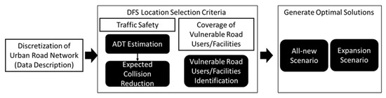
Figure 1.
Overview of the proposed framework.
3.2. Location Selection Criteria
To find the optimal installation sites for DFSs, two factors were considered within the framework. The first and top priority was the safety effectiveness (i.e., collision frequency reductions) that could be obtained from a certain implementation strategy. This factor was overwhelmingly used as the main deciding factor for site selection works that pertained to traffic safety countermeasures and/or facilities [16,24,38]. To quantify the expected collision frequency reductions for each candidate site, the equivalent-property-damage-only (EPDO) method was used to make a fair comparison between candidate sites by removing the collision severity and initial collision frequencies biases. This method is a weighting system where severe collisions receive the highest weightings and PDO collisions receive the least. Before estimating the expected safety effectiveness, the traffic volume (in our case, due to the data availability, average daily traffic (ADT) was used) value was interpolated using a geostatistical method for each site, which was critical to the whole framework.
The coverage of vulnerable road users and facilities was the second factor that needed to be included in the DFS site selection process [39]. The main reason why this was included in this framework was because of the special safety concern. Pedestrians, especially minors and seniors who experience a greater risk of injury in any collision with a vehicle, are therefore highly in need of protection against collisions [40]. For this study, vulnerable users and areas were represented by school zones, playgrounds, bus stops, and senior residences, which were combined as a factor to be utilized in the framework [38,41,42]. With different concerns in terms of the vulnerable road users/facilities (e.g., cyclists), this factor could also be updated.
Since there were two factors considered in the criteria, there would be no exclusive optimal implementation strategy overall. To integrate these two factors into the site selection process, the level of importance between the two factors needed to be adjusted by using a trade-off criterion. The criterion was determined by applying weights, where the greater the weight that is applied, the more importance that is placed on that factor. For each of the different criteria, both all-new and expansion scenarios were considered.
3.2.1. Traffic Safety
A set of locally developed safety performance functions (SPFs) and collision reduction ratios were established in our previous study [9], as summarized in Table 1, and the expected collision reduction was calculated for each candidate site via the Empirical Bayes (EB) method.

Table 1.
Overall before-and-after evaluation results from previous works [9].
The first step was to calculate the expected number of collisions in the before period for each site (i.e., road segment). The expected number of collisions in the before period was calculated as a weighted combination of the predicted number of collisions in the before period (from SPFs) adjusted by the yearly calibration factor (YCFs) and the observed number of collisions in the before period [43]. The model form of SPFs and YCFs used and calibrated in our previous studies is shown as Equations (1) and (2). Equations for calculating the expected number and weighted adjustment factor are shown as Equations (3) and (4) below. Here, the whole observation period for the untreated sites is the before period as there are no DFSs installed at those sites.
where is the predicted yearly average collision frequency; is the traffic volume, i.e., ADT of the road segment; is the length of the road segment in meters; , , and are the regression parameters; is the weighted adjustment factor (between 0 and 1); is the expected number of collisions in the before period; is the predicted number of collisions in the before period; is the observed number of collisions in the before period; is the overdispersion parameter estimated from SPF; is the yearly calibration factor.
Collisions for each candidate site were divided into two severity categories—PDO and severe—and the collision reductions were found for both. Once the expected collision reductions for both severities were found, they were then multiplied by the equivalent-property-damage-only (EPDO) weights and summed. An EPDO weight is defined as the ratio between the costs of a certain severity of a collision to a PDO collision [44]. Figure 2 is a flowchart showing the workflow for the computational process of this step.
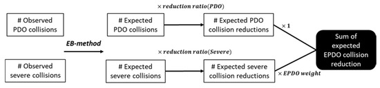
Figure 2.
Workflow of calculating equivalent-property-damage-only (EPDO) collision reductions.
The second step was to calculate the expected collision reductions for each site if it was treated with a DFS, which is represented by Equation (5).
where is the expected EPDO collision reduction for site i; represents the collision reduction ratio and can be found in Table 1; is the EPDO weight for a severe collision.
In order to use the EB method to calculate the expected collision frequencies, the corresponding estimated ADT data for that road segment were required, as will be discussed later in this paper.
3.2.2. Vulnerable Road Users and Facilities
In this framework, locations that have bus stops, nearby schools, playgrounds, and senior residences were considered vulnerable facilities or a source of vulnerable users. The ArcGIS developed by Esri [45] was used to as a primary data assimilation platform for processing the relevant geospatial data.
In ArcGIS, all the bus stops were assigned to their located road segments. Any road segments with a speed limit equal to or under 30 km/h were assumed to be near vulnerable road users/facilities, such as schools and playgrounds. For senior residences, a 500-m distance threshold was used to label road segments as being nearby a senior residence. Each of these three variables was a binary value, indicating it was either present or not. For each candidate segment, these three variables were summed to obtain a coverage value, thus the minimum coverage value would be 0 and the maximum would be 3. Outlined below are the following steps for this procedure.
Step 1: Map the segments with speed limits under or equal to 30 km/h, locations of senior residences, and bus stops.
Step 2: Intersect the segments where the speed limit is under or equal to 30 km/h with all the candidate segments. Intersected segments are considered close to schools, playgrounds, or other vulnerable road users/facilities and their attribute of coverage for schools/playgrounds will be set to 1, otherwise 0.
Step 3: Calculate the network distance between each senior residence and segment. If the distance is less than or equal to 500 m, then that segment is considered close to a senior residence. If a segment is identified to be close to at least one senior residence, the attribute of coverage for senior residences can be covered by the DFS in that segment will be set to 1, otherwise 0.
Step 4: Assign the bus stops into their located segments and count the number of bus stops located in each segment. If a segment has at least one bus stop, the attribute of coverage for bus stops located on that segment will be set to 1, otherwise 0.
Step 5: Add the results obtained in Steps 2–4 together for each candidate site. The maximum final value of coverage for vulnerable road users/facilities will be 3 and the minimum will be 0.
Step 6: Normalize the results obtained in Step 5 between 0 and 1 for all segments.
Both EPDO collision reductions and coverage of vulnerable road users/facilities were normalized between 0 and 1 to convert them into a dimensionless term to enforce a fair comparison. A weighted value was proposed to allow decision makers to adjust the level of importance on these two factors based on their specific needs. To find the optimal strategy for deploying DFSs in the city, the greedy algorithm was utilized to iteratively update the demand surfaces (i.e., safety conditions and coverage of vulnerable road users/facilities in each segment) by locating one DFS at a time and then comparing the segments’ objective values while under a series of constraints.
3.3. Traffic Volume Estimation via Kriging
As mentioned previously, traffic volume information is mandatory in estimating the traffic safety effects. A variety of techniques have been implemented to estimate traffic counts. Each method takes known traffic counts and uses additional information (e.g., land use, time-steps, road geometry attributes, etc.) to make a prediction [46]. These estimates can be separated into future-year and present-year predictions. Future-year predictions use current and past traffic count data to estimate the traffic count at a future date. On the other hand, current-year predictions use the traffic data available to estimate traffic counts at unmeasured locations. For this study, the average daily traffic (ADT) data were available at various locations for every year, therefore the current-year prediction method was used to interpolate yearly ADT values at unmeasured road segments.
Kriging is one of the most commonly used geostatistical spatial interpolation techniques that also account for the uncertainty of the estimation [47]. Kriging predicts the values at unsampled locations from the weighted average of nearby measured observations. Weights are determined based on their distance from the unsampled location and their closeness to each other. The basic equation of kriging is given as:
where is the estimated value at location , is the measured observations at the sampling site , is the kriging weight, and n is the number of sampling locations within the search neighborhood, and indicates expected values. The goal is to determine the optimal kriging weights that minimize the variance of the estimator under the unbiasedness constraint, . Kriging weights for each sampling location are estimated based on the parameters of the semivariogram model and the relative distance of the specific point with other sampling points and the unknown point [48,49]. Constructing a good quality semivariogram is a prerequisite to improving the accuracy of estimation results. In short, the semivariogram is the plot of the expected value of the semivariance of the variable of interest. It is a statistic that shows how the level of similarity between two known points decreases as their separation distance increases. Semivariogram modeling follows sophisticated processes that are worthy of a separate paper, and thus detailed descriptions are omitted in this paper. Readers interested in this topic are referred to more comprehensive modeling guidelines provided by [50]. Once the semivariograms are constructed for each year, kriging is used to interpolate the ADT values for all the unmeasured road segments.
In geostatistics, cross-validation is used to assure the accuracy of interpolated results. It is a statistical term that describes a unique verification process in which each observation is removed to produce an estimate at the same location of removal [50]. The goodness of fit is calculated using some statistical measures including mean standardized error (MSE) and root mean squared standardized error (RMSSE) to represent its robustness by examining, for instance, how closely the fitted model predicts the measured values. In this study, the Geostatistical Analyst package in Esri ArcGIS was used to construct semivariograms and perform spatial interpolation via kriging [45].
3.4. Problem Formulation
Once the expected EPDO collision reductions and coverage of vulnerable road users/facilities are determined and normalized, they can be included as the factors in the objective function of this framework. The objective function of locating DFSs is shown in Equation (7).
Subject to:
where is the objective value of all the selected sites by integrating collision reductions (first term) and coverage of vulnerable road users/facilities (second term); is the weight value (usually between 0 and 1) allowing users to place different levels of importance between the two factors (8); represents the total number of candidate sites; is a binary decision variable (0 or 1) that controls the selection of the ith candidate site, if is equal to 1, it means the ith candidate site is included, otherwise no (9); is a second decision variable representing whether the mth DFS is located in the ith candidate site (10); represents the maximum number of DFSs that can be located in the ith road segment, this number can be determined by the road segment length and the DFS placement interval; means the normalized collision reduction after putting the mth DFS into the ith candidate site; is the normalized coverage of vulnerable road users/facilities of the ith candidate site; is the total available budget (i.e., the total number of DFSs that will be located) (11).
3.5. Optimization via Greedy Algorithm
The greedy algorithm was utilized as the solution algorithm in this framework. The greedy algorithm follows the problem solving heuristic of making the locally optimal choice at each stage with the intent of finding a global optimum [51]. In many problems, a greedy strategy does not usually produce an optimal solution, but a greedy heuristic may yield locally optimal solutions that approximate a globally optimal solution in a reasonable amount of time. In our case, since the two factors in the objective function could be calculated in a deterministic way for each candidate site, the greedy algorithm was deemed suitable for application and thus implemented herein to find the optimal solutions. The workflow of the greedy algorithm is shown in Figure 3.
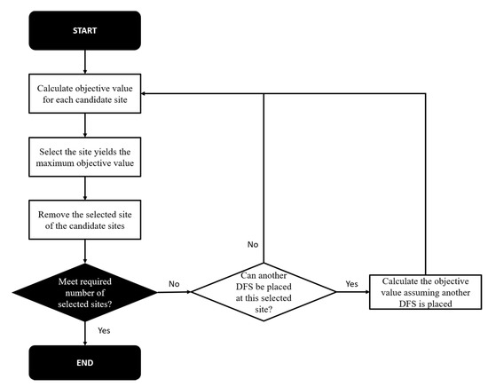
Figure 3.
Workflow of the greedy algorithm.
4. Case Study
4.1. Study Area
The study area focused primarily on arterial and collector road segments in the city of Edmonton, which is the capital city of the Canadian province of Alberta. The city has been installing DFSs as a traffic safety countermeasure since 2011, choosing locations based on historical collision records and documented speeding incidents. To date, there are 212 DFSs installed throughout the city in various areas (displayed in Figure 4), and 142 of them are installed in the study area (i.e., arterial and collector roads). The segmentation of arterial roads was based on end nodes that were composed of signalized intersections only while the segmentation on collector roads was based on end nodes that were intersections to either another collector or arterial for a total of 11,260 road segments. Historical collision data observed and collected between 2009 and 2018 were geocoded and assigned to each corresponding segment. The reported midblock collision frequencies can be found in Figure 5. It can be concluded, starting from 2011, the midblock collisions started to decline, which validates the safety effects of the DFSs. By following the procedures of the proposed framework, the follow section demonstrates the results for each part in detail.
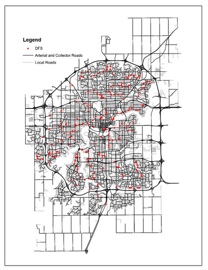
Figure 4.
Driver feedback sign (DFS) locations in the city of Edmonton.
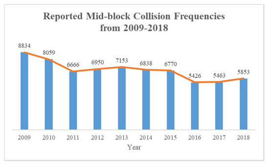
Figure 5.
Historical collisions from 2009 to 2018 in the city of Edmonton [9].
4.2. Results and Discussions
4.2.1. Interpolation of Missing ADT Values
Following the steps identified previously, one of the most well-adopted variants of kriging, namely, ordinary kriging (OK), was used to interpolate the missing ADT values for the candidate road segments for each year. The historical observed ADT data between 2009 and 2018 were also provided by the city of Edmonton; ADT detection sites can be found in Figure 6. Semivariograms for each year were calibrated and applied to interpolate missing ADT values over the entire study domain, among which the number of segments with interpolated ADT accounts for around 89.5% of total road segments, while the proportion of those with actual collected ADT accounts for 10.5%. Statistical analyses were followed to ensure the quality of each kriging model developed herein. The maps of the estimated ADT distributions from 2009 to 2018, excluding 2017 (due to insufficient data), are shown in Figure 7.
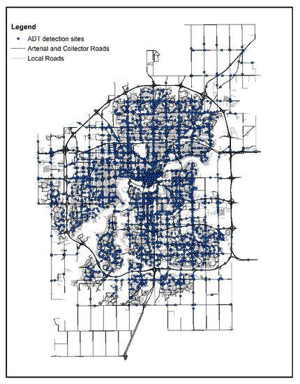
Figure 6.
Average daily traffic (ADT) detection sites.
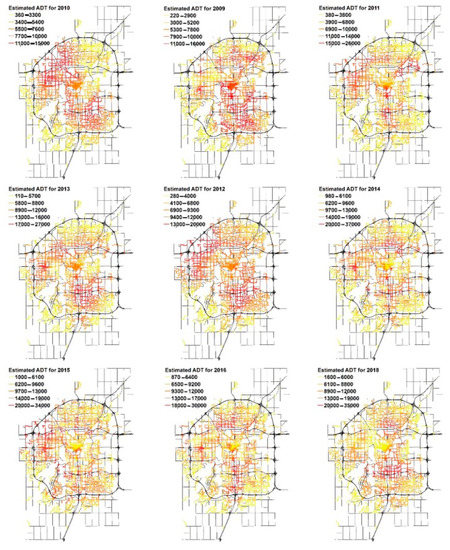
Figure 7.
Estimated ADT values in the city road network.
4.2.2. Mapping of Location Selection Criteria
Following the procedures introduced in Section 3.2, Location selection criteria, expected EPDO collision reductions and coverage of vulnerable road users/facilities were calculated and normalized for each candidate road segment. The EPDO weights used in this case study were calculated based on the estimated direct costs [52] for PDO and severe collisions. This information is shown in Table 2. Figure 8 is a map showing the locations of all these vulnerable facilities. The final resulting map of these two criteria is displayed in Figure 9.
Table 2.
Estimated collision costs and EDPO weights.
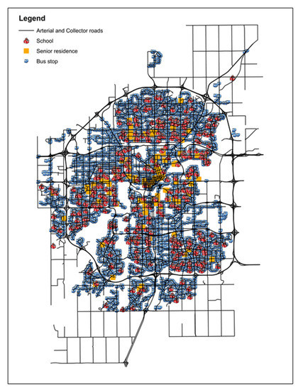
Figure 8.
Map of the vulnerable road users/facilities.
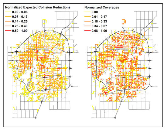
Figure 9.
Maps of normalized location selection criteria.
The two maps in Figure 9 illustrate that high expected collision reductions are more likely to occur in the city core areas where traffic volumes and historic collision frequencies are relatively higher. The maps also show that the coverages of vulnerable road users/facilities are widely distributed around the whole city rather than being clustered.
4.2.3. Citywide DFS Implementation Selection Criteria
With the selection criteria (safety and coverage) mapped for all candidate sites in the city areas, the DFS implementation strategies can be determined via employing the greedy algorithm to find the optimal solutions. Another input required in the framework is the DFS placement interval. Since limited literature exists on the halo effects of DFSs in urban networks, the halo effect of a mobile photo enforcement (MPE) study [53] using a 1-km distance was set as the distance interval between DFSs (i.e., DFS units cannot be installed less than 1 km from each other). This was intuitive, since both MPE and DFSs have several similarities between them, and the MPE study was also conducted in the city of Edmonton. In addition, in terms of the real engineering concerns, Edmonton’s city blocks are usually around 100 m [54], thus the reasoning for segments with lengths longer than one kilometer or shorter than 100 m were excluded from the candidate sites. Highway road segments were also excluded since DFSs mainly target reducing collisions on arterial and collector roads. Ultimately, there were 6277 candidate sites (including 142 sites with DFSs already installed) that met the requirements for the study and were included in the framework for DFS location and allocation.
All-New Scenario
The all-new scenario is a hypothetical simulation of relocating all existing DFSs in the study area to compare the objective value of the existing deployment with that of the theoretical optimal deployment strategy. The results can be used to assess the current deployment strategy of DFSs and benchmark an optimal criterion.
In this study, three different weights were used to generate strategies by placing different importance on safety effectiveness () and coverage of vulnerable road users/facilities (). The total budget constraint was assumed to be equivalent to the number of existing DFSs currently in place (i.e., 142 out of 212) in the city of Edmonton. The optimization formulated earlier was implemented to locate DFSs such that traffic safety and coverage of vulnerable facilities and users could be maximized. The optimal site locations generated via the greedy algorithm are shown in Figure 10, with the street views for three selected sites of the 0.5-weight value displayed to portray how well the proposed optimizer delineated locations that are prone to accidents (e.g., sites 1 and 2) and vulnerable facilities (e.g., sites 3).
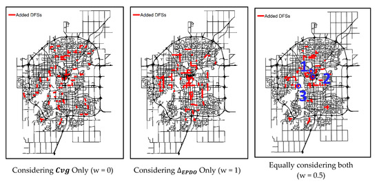
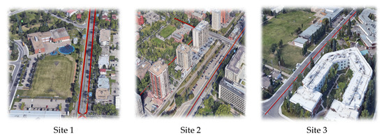
Figure 10.
Selected sites distribution of all-new scenario.
It can be observed that the distribution of the selected DFS sites changed based on the weightings applied to each of the factors. As the weight applied to the safety effectiveness () increased, so did the preference for locating DFSs at high collision sites. By contrast, as the weighting value was reduced, then the preference shifted to cover more sites identified as vulnerable facilities or zones with vulnerable users.
Using the existing deployment as a point of reference, Table 3 shows how the level of improvements in percentage (negative value means decrease) on the reduction of collisions and coverage of vulnerable road users/facilities changed as the weights changed. As expected, as the weight value increased (i.e., more importance placed on collision reduction), the level of improvement for collision reduction increased, while the coverage of vulnerable road users/facilities decreased, and vice versa. For example, when the weight value was set to 0, the optimal DFS locations were selected for maximizing the . As a result, when compared with the current DFS deployment, the optimal one led to 38.1% less but 69.27% more . The results of this comparison show that the current DFS deployment strategy focuses more on zones with high collision rates but still has room for improvement if the optimal deployment strategy is adopted.
Table 3.
Percentage change based on all-new scenario.
Expansion Scenario
While the results from the all-new scenario showed that the current deployment could be improved, relocating the entire set of existing DFSs was not an economically feasible option as it would entail a laborious and timely endeavor. Therefore, this section details a way to expand the system by adding more DFSs to the existing deployment scheme. The optimization procedure introduced earlier was modified to reflect the changes in the base condition. The objective function was evaluated at each iteration by considering the fixed DFSs throughout the entire optimization process. Identical optimization parameters and weighting schemes were used to generate optimal location solutions. The locations of the selected sites for an additional 10 and 20 DFSs are shown in Figure 11 with some of the street views of the selected sites of the expansion scenarios using the weight value of 0.5. This further confirmed that the results generated from this framework met expectations as some of the sites were near schools, playgrounds, and senior residences, while others were placed in areas with a high collision frequency.
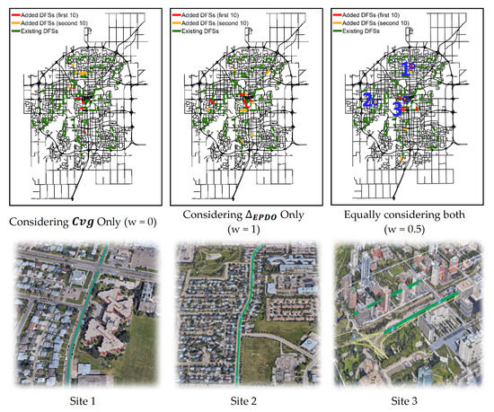
Figure 11.
Sites selected for 10–20 future DFSs.
Similar to the all-new scenario, the same trend in the distribution of selected sites based on the weightings can be seen in this expansion scenario. As before, the level of improvements based on weightings was found in both examples of adding 10 or 20 additional DFSs, and these are shown in Table 4. Again, these statistics followed the same trend that was observed with the all-new scenario, with the only difference being that there were no negative improvement values.
Table 4.
Percentage change based on expansion scenario.
5. Conclusions, Limitations and Future Research
This study expanded the discussion on a location-allocation framework for a citywide DFS implementation. The EB method with locally constructed SPFs and estimated ADT was utilized as part of the EPDO method to calculate the expected collision reductions for each candidate site as a result of installing a DFS. Another location selection criterion considering vulnerable road users/facilities was spatially processed and distributed to each site via ArcGIS.
For the first time in the literature, this study developed a formal mathematical programming approach that aims at designing citywide optimal DFS implementation strategies by considering its effects on traffic safety and vulnerable road users. This framework can be easily duplicated and utilized in other cities for similar traffic safety countermeasures. The findings were supported by the results from the improvement comparisons and the sites that were selected based on which factor was deemed more important. As the weight value increased from 0 to 1, the level of importance shifted in favor of reducing collisions over coverage of vulnerable road users/facilities. The opposite was true when the weight value decreased from 1 to 0, favoring coverage of vulnerable road users/facilities over collision reduction, thus making school zones, playgrounds, and senior residences a more favorable site for DFS intervention.
The all-new scenario results revealed that the current DFS deployment in the city of Edmonton focuses more on areas with a high collision frequency. The differences between the suggested optimal locations and current locations indicated that the benefits obtained from DFSs can be improved significantly by redesigning the current deployment. The collision reductions and coverage of vulnerable road users/facilities can be improved by up to 149.4% or 69.27%, respectively, if the level of importance was assigned accordingly.
The expansion scenario resulted in a list of optimal sites that can be considered for future DFSs. The change in the location distributions and improvements based on different weight values given to them matched the expectations and the real situation as observed in the city. The results indicated that collision reductions can be improved by up to 30.22% or 51.61% when adding 10 or 20 more DFSs, respectively, while the coverage of vulnerable road users/facilities can be improved by up to 14.63% or 29.27%, respectively.
Overall, the findings of this study suggest that the proposed DFS location-allocation framework is simple and convenient to implement as it provides decision makers with the freedom to simulate and optimize their DFS network by balancing the needs of the road users, vulnerable facilities, and traffic safety in locating DFS over an urban road network.
Although a site selection framework was developed to provide a system optimal implementation strategy for future DFS locations, it is still unknown how many DFSs would be required in urban areas. Besides, the DFS is not the only countermeasure used in speed control, the combined use of DFS and other countermeasures, such as intersection safety device (ISD) and mobile photo enforcement (MPE), may alter the location-allocation strategies. Therefore, this research can be further refined and investigated in several directions.
First, there may be a diminishing return to the safety benefit as more and more DFSs are added and, eventually, the improvements would benefit coverage levels more than safety. Since there are limited resources for expanding the DFS program, it will be meaningful to investigate the optimal density or optimal number of DFSs needed in the future.
Second, the mutual effects between DFSs and other countermeasures are unknown. Since the cities may also plan to expand existing ISD and MPE programs to make the urban network safer, it will be necessary to create a comprehensive assessment system that would consider these three countermeasures together, rather than individually, when an expansion strategy is in its planning phase. This means the system optimal implementation strategy would be generated not by separating these countermeasures into individual parts but by integrating them as a whole. This additional research will expand the existing body of knowledge on the development of sustainable DFS location-allocation strategies that will improve the effectiveness and efficiency of future traffic safety programs.
Third, to better interpolate traffic volumes at unmeasured locations, more advanced kriging variants, such as network kriging or kriging with external drifts, should be explored to take into account additional covariates such as the number of lanes and types of roads (e.g., arterials, collectors) to further improve the model performance. This has the potential for obtaining a greater level of accuracy of the estimation results.
Nevertheless, the DFS location-allocation framework developed herein was able to provide reliable deployment strategies based on two different weighting schemes such that DFS planners could easily be able to adjust the level of importance based on their needs and use for real-world applications. Furthermore, with this decision support system in hand, the city officials will be able to improve upon existing policies in an attempt to further reduce speed-related collisions.
Author Contributions
The authors confirm contribution to the paper as follows: study conception and design: M.W., T.J.K., K.E.-B.; data collection and process: M.W.; analysis and interpretation of results: M.W., T.J.K., K.E.-B.; draft manuscript preparation: M.W., T.J.K., K.E.-B. All authors have read and agreed to the published version of the manuscript.
Funding
This research was funded by the City of Edmonton’s Traffic Safety Section, Alberta, Canada.
Acknowledgments
The authors would like to acknowledge the financial support and guidance from the city of Edmonton’s Traffic Safety Section, Alberta, Canada.
Conflicts of Interest
The authors declare no conflict of interest.
References
- World Health Organization. Global Status Report on Road Safety 2013: Supporting a Decade of Action: Summary; World Health Organizatio: Geneva, Switzerland, 2013. [Google Scholar]
- European Conference of Ministers of Transport; OECD/ECMT Transport Research Centre, Speed Management; OECD Publishing: Pairs, France, 2006.
- Transport Canada. Road Safety in Canada. 2011. Available online: https://www.tc.gc.ca (accessed on 20 November 2019).
- McCoy, P.T.; Bonneson, J.A.; Kollbaum, J.A. Speed reduction effects of speed monitoring displays with radar in work zones on interstate highways. Transp. Res. Rec. 1995, 1509, 65–72. [Google Scholar]
- Garber, N.J.; Patel, S.T. Effectiveness of Changeable Message Signs in Controlling Vehicle Speeds in Work Zones; Virginia Transportation Research Council: Charlottesville, VA, USA, 1994. [Google Scholar]
- Fontaine, M.D.; Carlson, P.J. Evaluation of speed displays and rumble strips at rural-maintenance work zones. Transp. Res. Rec. 2001, 1745, 27–38. [Google Scholar] [CrossRef]
- Lee, C.; Lee, S.; Choi, B.; Oh, Y. Effectiveness of speed-monitoring displays in speed reduction in school zones. Transp. Res. Rec. 2006, 1973, 27–35. [Google Scholar] [CrossRef]
- Rose, E.R.; Ullman, G.L. Evaluation of Dynamic Speed Display Signs (DSDS); Texas Transportation Institute: San Antonio, TX, USA, 2003.
- Wu, M.; El-Basyouny, K.; Kwon, T.J. Before-and-after empirical Bayes evaluation of citywide installation of driver feedback signs. Transp. Res. Rec. 2020, 2674, 419–427. [Google Scholar] [CrossRef]
- Wu, M.; El-Basyouny, K.; Kwon, T.J. Lessons learned from the large-scale Application of Driver Feedback Signs in an urban city. J. Transp. Saf. Secur. 2020, 1–19. [Google Scholar] [CrossRef]
- Ullman, G.L.; Rose, E.R. Evaluation of Dynamic Speed Display Signs. Transp. Res. Rec. 2005, 1918, 92–97. [Google Scholar] [CrossRef]
- Santiago-Chaparro, K.R.; Chitturi, M.; Bill, A.; Noyce, D.A. Spatial Effectiveness of Speed Feedback Signs. Transp. Res. Rec. 2012, 2281, 8–15. [Google Scholar] [CrossRef]
- Williamson, M.R.; Fries, R.N.; Zhou, H. Long-Term Effectiveness of Radar Speed Display. J. Transp. Technol. 2016, 6, 99–105. [Google Scholar]
- Effectiveness of Changeable Message Signs in Controlling Vehicle Speeds in Work Zones: Phase II. 1998. Available online: https://trid.trb.org/view/473832 (accessed on 20 November 2019).
- Mattox, J.H.; Sarasua, W.A.; Ogle, J.H.; Eckenrode, R.T.; Dunning, A. Development and Evaluation of Speed-Activated Sign to Reduce Speeds in Work Zones. Transp. Res. Rec. 2007, 2015, 3–11. [Google Scholar] [CrossRef]
- Kwon, T.J. Development and Evaluation of Models and Algorithms for Locating RWIS Stations. Ph.D. Thesis, University of Waterloo, Waterloo, ON, Canada, 2015. [Google Scholar]
- Hakimi, S.L. Optimum Locations of Switching Centers and the Absolute Centers and Medians of a Graph. Oper. Res. 1964, 12, 450–459. [Google Scholar] [CrossRef]
- Hakimi, S.L. Optimum distribution of switching centers in a communication network and some related graph theoretic problems. Oper. Res. 1965, 13, 462–475. [Google Scholar] [CrossRef]
- ReVelle, C.; Eiselt, H.; Daskin, M. A bibliography for some fundamental problem categories in discrete location science. Eur. J. Oper. Res. 2008, 184, 817–848. [Google Scholar] [CrossRef]
- Owen, S.H.; Daskin, M.S. Strategic facility location: A review. Eur. J. Oper. Res. 1998, 111, 423–447. [Google Scholar] [CrossRef]
- Daskin, M.S. Network and Discrete Location: Models, Algorithms, and Applications; John Wiley & Sons: Hoboken, NJ, USA, 2011. [Google Scholar]
- ReVelle, C.; Toregas, C.; Falkson, L. Applications of the Location Set-covering Problem. Geogr. Anal. 1976, 8, 65–76. [Google Scholar] [CrossRef]
- Lim, S.; Kuby, M. Heuristic algorithms for siting alternative-fuel stations using the Flow-Refueling Location Model. Eur. J. Oper. Res. 2010, 204, 51–61. [Google Scholar] [CrossRef]
- Jin, P.J.; Walker, A.; Cebelak, M.; Walton, C.M. Determining Strategic Locations for Environmental Sensor Stations with Weather-Related Crash Data. Transp. Res. Rec. 2014, 2440, 34–42. [Google Scholar] [CrossRef]
- Church, R.; ReVelle, C. The maximal covering location problem. Pap. Reg. Sci. Assoc. 1974, 32, 101–118. [Google Scholar] [CrossRef]
- Suzuki, A.; Drezner, Z. The p-center location problem in an area. Locat. Sci. 1996, 4, 69–82. [Google Scholar] [CrossRef]
- Balinski, M.L. Integer Programming Methods, Uses, Computation. Manag. Sci. 1965, 12, 253–313. [Google Scholar] [CrossRef]
- Kuby, M.J. Programming Models for Facility Dispersion: The p-Dispersion and Maxisum Dispersion Problems. Geogr. Anal. 1987, 19, 315–329. [Google Scholar] [CrossRef]
- Dell’Olmo, P.; Ricciardi, N.; Sgalambro, A. A multiperiod maximal covering location model for the optimal location of intersection safety cameras on an urban traffic network. Procedia-Soc. Behav. Sci. 2014, 108, 106–117. [Google Scholar] [CrossRef]
- Garey, M.R.; Johnson, D.S. Computers and Intractability: A Guide to the Theory of NP-Completeness. In Bulletin (New Series) of the American Mathematical Society; American Mathematical Society: Providence, RI, USA, 1980. [Google Scholar]
- Mahdian, M.; Markakis, E.; Saberi, A.; Vazirani, V. A Greedy Facility Location Algorithm Analyzed Using Dual Fitting. In Approximation, Randomization, and Combinatorial Optimization: Algorithms and Techniques; Springer: Berlin/Heidelberg, Germany, 2001. [Google Scholar]
- Cormen, T.H.; Leiserson, C.E.; Rivest, R.L.; Stein, C. Introduction to Algorithms; MIT Press: Cambridge, MA, USA, 2001. [Google Scholar]
- Van Laarhoven, P.J.; Aarts, E.H. Simulated annealing. In Simulated Annealing: Theory and Applications; Springer: New York, NY, USA, 1987. [Google Scholar]
- Goldberg, D.E. Computer-Aided Gas Pipeline Operation Using Genetic Algorithms and Rule Learning. Ph.D. Thesis, University of Michigan, Ann Arbor, MI, USA, 1984. [Google Scholar]
- Eberhart, R.C.; Kennedy, J. Particle swarm optimization. In Proceedings of the ICNN’95-International Conference on Neural Networks, Perth, WA, Australia, 27 November–1 December1995; Volume 4, pp. 1942–1948. [Google Scholar]
- Davidović, T.; Ramljak, D.; Šelmić, M.; Teodorović, D. Bee colony optimization for the p-center problem. Comput. Oper. Res. 2011, 38, 1367–1376. [Google Scholar] [CrossRef]
- Geem, Z.W.; Kim, J.H.; Loganathan, G. A New Heuristic Optimization Algorithm: Harmony Search. Simulation 2001, 76, 60–68. [Google Scholar] [CrossRef]
- Kim, A.M.; Wang, X.; El-Basyouny, K.; Fu, Q. Operating a mobile photo radar enforcement program: A framework for site selection, resource allocation, scheduling, and evaluation. Case Stud. Transp. Policy 2016, 4, 218–229. [Google Scholar] [CrossRef]
- Li, M.; Faghri, A.; Fan, R. Determining Ideal Locations for Radar Speed Signs for Maximum Effectiveness: A Review of the Literature; Delaware Center for Transportation: Newark, NJ, USA, 2017. [Google Scholar]
- Constant, A.; Lagarde, E. Protecting Vulnerable Road Users from Injury. PLoS Med. 2010, 7, e1000228. [Google Scholar] [CrossRef]
- Li, Y.; Kim, A.; El-Basyouny, K. Scheduling resources in a mobile photo enforcement program. In Proceedings of the 2017 4th International Conference on Transportation Information and Safety (ICTIS), Banff, AB, Canada, 8–10 August 2017. [Google Scholar]
- Li, Y.; Xie, J.; Kim, A.M.; El-Basyouny, K. Investigating trade-offs between optimal mobile photo enforcement programme plans. J. Multi-Criteria Decis. Anal. 2019, 26, 51–61. [Google Scholar] [CrossRef]
- Li, R.; El-Basyoung, K.; Kim, A. Before-and-after empirical Bayes evaluation of automated mobile speed enforcement on urban arterial roads. Transp. Res. Rec. J. Transp. Res. Board 2015, 2516, 44–52. [Google Scholar] [CrossRef]
- Rodegerdts, L.A.; Nevers, B.L.; Robinson, B.; Ringert, J.; Koonce, P.; Bansen, J.; Nguyen, T.; McGill, J.; Stewart, D.; Suggett, J.; et al. Signalized Intersections: Informational Guide; US Department of Transportation: Washington, DC, USA, 2004.
- ESRI ArcGIS. Release 10; Environmental Systems Research Institute: Redlands, CA, USA, 2011.
- Selby, B.; Kockelman, K.M. Spatial Prediction of AADT in Unmeasured Locations by Universal Kriging. 2011. Available online: https://trid.trb.org/view/1092064 (accessed on 20 November 2019).
- Cressie, N. The origins of kriging. Math. Geol. 1990, 22, 239–252. [Google Scholar] [CrossRef]
- Lichtenstern, A. Kriging Methods in Sptial Statistics. Bachelor’s Thesis, Technical University of Munich, München, Germany, 2013. [Google Scholar]
- Kwon, T.J.; Fu, L. Spatiotemporal variability of road weather conditions and optimal RWIS density—An empirical investigation. Can. J. Civ. Eng. 2017, 44, 691–699. [Google Scholar] [CrossRef]
- Olea, R.A. A six-step practical approach to semivariogram modelling. Stoch. Environ. Res. Risk Assess. 2006, 20, 307–318. [Google Scholar] [CrossRef]
- Bird, R.; De Moor, O. From dynamic programming to greedy algorithms. In Formal Program Development; Springer: Berlin/Heidelberg, Germany, 1993. [Google Scholar]
- De Leur, P. Collision Cost Study Update FINAL Report. 2018. Available online: https://drivetolive.ca/wp-content/uploads/2020/07/CollisionCostStudyUpdate_FinalReport.pdf (accessed on 11 December 2020).
- Gouda, M.; El-Basyouny, K. Investigating Distance Halo Effects of Mobile Photo Enforcement on Urban Roads. Transp. Res. Board 2017, 2660, 30–38. [Google Scholar] [CrossRef]
- City of Edmonton. City Design and Construction Standards. 2019. Available online: https://www.edmonton.ca/ (accessed on 20 November 2019).


Publisher’s Note: MDPI stays neutral with regard to jurisdictional claims in published maps and institutional affiliations. |
© 2020 by the authors. Licensee MDPI, Basel, Switzerland. This article is an open access article distributed under the terms and conditions of the Creative Commons Attribution (CC BY) license (http://creativecommons.org/licenses/by/4.0/).