Abstract
Finding trees that are resistant to pathogens is key in preparing for current and future disease threats such as the invasive white pine blister rust. In this study, we analyzed the potential of using hyperspectral imaging to find and diagnose the degree of infection of the non-native white pine blister rust in southwestern white pine seedlings from different seed-source families. A support vector machine was able to automatically detect infection with a classification accuracy of 87% (κ = 0.75) over 16 image collection dates. Hyperspectral imaging only missed 4% of infected seedlings that were impacted in terms of vigor according to expert’s assessments. Classification accuracy per family was highly correlated with mortality rate within a family. Moreover, classifying seedlings into a ‘growth vigor’ grouping used to identify the degree of impact of the disease was possible with 79.7% (κ = 0.69) accuracy. We ranked hyperspectral features for their importance in both classification tasks using the following features: 84 vegetation indices, simple ratios, normalized difference indices, and first derivatives. The most informative features were identified using a ‘new search algorithm’ that combines both the p-value of a 2-sample t-test and the Bhattacharyya distance. We ranked the normalized photochemical reflectance index (PRIn) first for infection detection. This index also had the highest classification accuracy (83.6%). Indices such as PRIn use only a small subset of the reflectance bands. This could be used for future developments of less expensive and more data-parsimonious multispectral cameras.
1. Introduction
Forest pests and pathogens have a harmful impact on forest structure, biodiversity, and function [1,2,3,4]. High mortality from non-native pathogens and pests has already occurred in several forest species [5]. Future projections identify 41.1% of total live forest biomass at risk in the US [6].
To prepare for these impacts, screening of trees for genetic resistance and susceptibility to pathogens and pests is important [7,8,9,10]. Forest managers can focus their resources where the infection is detected. They can anticipate the impacts of climate change by favoring both genetic diversity and more pest-resistant genotypes during restoration and reforestation [9].
Traditional methods for screening trees for resistance to a pathogen rely on large-scale common garden approaches [8,11]. These approaches can be laborious and time-consuming due to the need for individual assessment of many thousands of seedlings for disease symptoms and related traits. Furthermore, this is a manual process, which introduces an expert’s bias. An automatic phenotyping and disease-screening process could potentially increase efficiency and reduce costs.
Hyperspectral imaging (HSI) can facilitate large-scale disease detection. A hyperspectral camera measures the reflectance in multiple (usually >100) spectrally narrow bands. Examples of successful disease detection by HSI can be found for citrus greening [12] and in wheat stem rust [13]. In both cases, disease detection exceeded 80% accuracy. Early detection of stress caused by diseases is another well-studied topic; examples include red leaf blotch disease [14], Verticillium wilt [15,16], sugar beet disease [17,18], and potato blight [19]. Studies to detect differences in disease resistance among genotypes is an emerging application in hyperspectral imaging [7,20,21]. Many studies have focused on HSI for disease detection in crops. However, phenotyping forestry species, and specifically conifers, using HSI is lacking [22].
Southwestern white pine (Pinus strobiformis Engelm.), hereafter SWWP, is being threatened by a fungal pathogen. Efforts towards finding resistance within populations in field trials are ongoing. An automated phenotyping method such as HSI would be highly beneficial in terms of efficiency. SWWP is one of nine species of the white pine group (Pinus subgenus strobus) in North America that is highly susceptible to the non-native white pine blister rust caused by the fungal pathogen Cronartium ribicola J. C. Fisch. [23,24,25,26]. SWWP is endemic to the southwestern United States and Mexico. It is an intermediate shade-tolerant species and a component of mixed conifer forests [27]. Spores of C. ribicola enter the pine through needle stomata. The fungal mycelium spreads along the length of the needle before infecting branches or the bole of the tree where it disrupts vascular transport through canker formation. Lesions (spots) and chlorotic tissue form in the needles. There is a large variation in the number and size of needle spots, as well as differences in spot color on needles of infected plants [28]. In some cases, individual shedding of infected needles can occur. Infected needles may have reduced photosynthetic performance, as found in eastern white pine (P. strobus) [29].
We assessed the potential of hyperspectral imaging for automated and objective plant health assessment in genetic resistance trials for forestry applications. We conducted a study on SWWP seedlings infected with white pine blister rust. Our specific objectives were to (i) distinguish inoculated seedlings from non-inoculated control seedlings, and to (ii) identify seedling vigor status. Subsequently, we investigated what additional information HSI could provide. We determined which wavelengths and other hyperspectral features (vegetation indices (VIs) and band combinations) were most useful to separate (i) inoculated from non-inoculated control and (ii) assigned vigor classes. Finally, we developed a simple search algorithm to quickly identify hyperspectral features of interest.
2. Materials and Methods
Seedlings were grown in a greenhouse for eight months before half were inoculated with C. ribicola. Visual inspections of vigor class started immediately hereafter. Hyperspectral imaging started 7 months after inoculation. Spectral reflectance per tree was used to classify seedlings for inoculation and for vigor class to assess the potential of using hyperspectral instead of expert inspections. Moreover, we developed a search algorithm to rank the usefulness of hyperspectral features to separate for inoculation and vigor class.
2.1. Experimental Set-Up
Open-pollinated seed-bearing cones were collected from 10 parent trees spanning the biogeographic range and climatic zones of SWWP (Supplementary Material, Table S1). Seeds extracted from the cones of the maternal trees were sown in January 2017 at the United States Department of Agriculture’s Dorena Genetic Resource Center (DGRC) (Cottage Grove, OR, USA). Seedlings were grown for one growing season in supercell Cone-tainersTM (Ray Leach, Canby, OR, USA) (164 cm3) in half-sibling progeny blocks (hereafter, ‘family’) in the DGRC greenhouse. Each family consisted of 8 to 20 seedlings, with a total of 175 seedlings (Table S1).
Half of the seedlings were inoculated on 31 August 2017 with basidiospores of the rust fungus, C. ribicola, using standard inoculation procedures [24,30,31]. Mean inoculum target-density was 5000 spores/cm2, measured by the settlement of spores on glass slides positioned throughout the canopy. Spore germination rate exceeded 99%. The remaining half of the seedlings were reserved as non-inoculated controls and were not placed in the inoculation chamber. These control seedlings remained uninfected because the fungus needs a secondary host (Ribes) to spread, which was not present in the greenhouse.
Seedlings were transferred to a climate-controlled greenhouse at Oregon State University in October 2017. The greenhouse had an average day/night air temperature of 12/33 °C and relative humidity of 13/86%. The seedlings were transplanted into 7.5 L pots with a Metro Mix #840PC growth medium (Sun Gro Horticulture Canada Ltd., Agawam, MA, USA). The arrangement of pots on the greenhouse bench was randomized. Pots were watered to field-capacity twice weekly.
2.2. Vigor Assessments of Seedlings Inoculated with White Pine Blister Rust
Expert visual inspection of disease symptoms began on 16 November 2017 and proceeded approximately monthly until 12 October 2018. Each inoculated seedling was assigned a vigor ranking that included 1 for vigorous growth, 2 for moderately vigorous growth, 3 for sickly, and 4 for dead from white pine blister rust. The non-inoculated control seedlings were labeled 0. Three seedlings were omitted from further analysis because they died from other causes. Two additional seedlings were omitted because of uncertainty in placement. Hyperspectral imagery was captured within 4 days of all visual inspections starting in March 2018.
2.3. Hyperspectral Image Acquisition
The imagery was captured on 16 dates, starting in March 2018, and ending in October 2018. The time between capture dates varied from 2 days to 6 weeks and was altered according to the rate of change of symptom expression.
Images were captured using a Nano VNIR Hyperspec camera (400–1000 nm, Headwall Photonics, MA, USA). The camera was fitted with an 8 mm lens with a 30.4° field of view (FOV). It captured data in 271 bands and 12-bit radiometric resolution with a FWHM, full width half maximum, of 6 nm. Data were captured at nadir using a custom-built motion-control system [32], Figure S1.
Natural light was used for illumination. During the months of June–October, the outside of the greenhouse was covered with a light-diffusing coating, resulting in reduced shading within the canopy from direct sunlight. Analysis of reflectance from a 99% reflective reference panel determined that there were no absorption bands due to the diffusive coating. The exposure time of the camera was adjusted for each image capture to match the light intensity and avoid oversaturation of the signal returned by the reflectance reference panel.
2.4. Hyperspectral Image Processing
Data were converted to radiance using both the sensor-specific calibration and a dark reference image using SpectralView (version 5.5.1., Headwall Photonics, MA, USA). The reflectance was determined using the 99%-reflectance panel placed in the scene using the empirical line conversion [33].
2.5. Hyperspectral Target Extraction
A feature of hyperspectral imagery is the clear distinction between green foliage, background soil, and man-made surfaces. Pixels that contained plant foliage were automatically segmented from the background using a supervised classification in Matlab R2018b (MathWorks, Natick, MA, USA). Individual pots were identified within each image using a circle-detection function ‘imfindcircles’. Pots could then be identified based upon the location on the bench. All pixels belonging to a specific plant were identified, and the median reflectance at each wavelength was determined.
2.6. Hyperspectral Features
Changes in biochemical and biophysical properties of the plant, such as a decline in photosynthetic performance, can be estimated with indices derived from the reflectance spectrum. We used 84 VIs from literature (Table S2) organized in sub-categories such as chlorophyll and xanthophyll indices. Moreover, we also established band combinations, including normalized differential index (standard [34] and inversed logarithmic [35]); the simple ratio [36]; and the first derivatives [37].
Features in this study are considered all hyperspectral derived variables, including the median reflectance per spectral band, VIs, and other band combinations. There are known correlations between spectral features and physiological and biochemical processes in vegetation which we leveraged to understand the impact of the fungal disease better without physiological measurements.
2.7. Classification
The median reflectance and the 84 VIs (Table S2) were used as the input for the classification tasks. The first classification task was to find inoculated seedlings and secondly to separate seedlings into vigor classes (obtained from the visual assessments). Here we used a supervised support vector machine algorithm (SVM) with a linear kernel to classify seedlings into the two and five categories, respectively. Haagsma et al., (2020, in preparation) showed that this machine learning algorithm performed the best on average when comparing it to the performance of 22 classification models.
For both classification tasks, the fitness of the trained models was assessed by their overall accuracy and kappa-coefficient derived from a 10-fold cross-validation. Because the data were randomly split into groups for the 10-fold cross-validation, results may vary for every initiation of the machine learning algorithm. Therefore, we repeated this training 19 times to achieve robust results. The final categorization of each seedling was based on a majority vote, hence the need for an odd number of repetitions. The overall accuracy was calculated by summing the number of correctly classified seedlings in all classes and dividing it by the total number of seedlings. In addition, the probability of detection was calculated by taking the number of seedlings correctly identified as being infected and dividing it by the total number of infected seedlings.
Moreover, for the multi-class problems, the entire confusion matrix was reported. We included the probability of detection, the precision (the number of accurately identified seedlings in a class divided by the number of seedlings predicted to be in that particular class), and Cohen’s kappa coefficient of agreement [38]. The confusion matrix only reports on the final labels, and consequently does not reflect the certainty or score of each label. Therefore, we also reported the area under the receiver operating characteristic curve, AUC [39], for vigor classification. An AUC of 1 meant that there was no confusion between a true-positive and false-positive rate. The model was capable of distinguishing the current class from the other classes, i.e., a perfect score. An AUC of 0.5 was indicative of a poorly performing model, where the rate of true-positives was equal to the rate of false-positives.
2.8. Statistical Analysis to Assess Feature Importance
Classification algorithms are superior to simpler statistical analyses in terms of finding patterns in data and thus being able to assess which hyperspectral feature contains the most information to separate the classes. However, this advantage comes with a computational cost which increases with the number of features that are included. For example, on our machine (with an Intel Xeon CPU E3-1505M v5 @2.80 GHz, Santa Clara, CA, USA), classifying one feature with 170 observations takes 20 s. Assessing all features (~150,000) would take ~42 days. We, therefore, developed a novel search algorithm that was simpler and required less computational effort by using two statistical indicators of separation. First, for each feature, we performed a 2-sample t-test between two distributions (inoculated and control) or a one-way ANOVA between more than two distributions (vigor classes). We used the p-value as an indicator of the degree of separation between the means of the distributions. The second indicator was the Bhattacharyya distance (BD), a measure of closeness between the two distributions (inoculated and control) [40]. Both indicators were used in the ‘new search algorithm’ that was validated using the 84 VIs. We assumed that these represented the entire population of features but offered a small enough sample size to sufficiently validate this method against the classification accuracy from a linear SVM performed on each of the VIs. We ranked the importance of the VIs based on p-values and BD-values in two steps, see Figure S2 for a schematic workflow. First, the ith (for I = 1:n) ranked VIs based on p-value and on BD were identified, returning two VIs. Next, these VIs were ranked relative to each other based on the rank of the other indicator. For example, the first ranked based on BD was VI-A and on p-value was VI-B. Now we knew that VI-A and VI-B needed to go in the first and second slot, but we did not know in which order. We then looked at the rank that both VIs had in the other statistical indicator. For example, if VI-A’s rank in the p-value was 12 and VI-B’s rank for BD was 8, then the final order should be VI-B first and then VI-A (8 < 12). Hereafter, we applied minimum criteria (BDi > median(BD) and pi < median(p)) for each of the VIs to filter for outliers. Note that Bhattacharyya distance can only be calculated for two distributions. Thus, for ranking features for separation in vigor class, we only used p-values.
The search algorithm was tested on the entire data set, as well as two subsets taken from an early and late time period to assess if there was a time dependency on the effectiveness of the algorithm to identify informative features. For the early time period, the variables were averaged over the first four acquisition dates, during which the vigor of ≤32% of the inoculated seedlings was impacted. For the late-stage time period, variables were averaged over the last four acquisition dates, when the vigor of 72% or more of the inoculated seedlings was negatively affected.
For vigor class assessment, a probabilistic multinomial regression was used to calculate the probability density function to determine the power of separation using the most informative VI. All analyses were conducted with Matlab’s Statistics and Machine Learning Toolbox R2018b (Mathworks, Natick, MA, USA).
Reflectance hypercubes and metadata are available from Oregon State University’s Scholars Archive [41]. Codes used for data processing and analysis are available from https://github.com/MarjaH/SWWP-infection-detection.
3. Results
3.1. Visual Assessments of White Pine Blister Rust
Inoculation was successful; 100% of inoculated seedlings developed needle spots, the first visual indicator of infection. Seedlings from the diverse families differed in reaction to the pathogen infection in terms of vigor impact and timing (Figure 1). Mortality ranged from 0 to 100%. Families B and D (families with suspected major gene resistance), and even A, had a large fraction of vigorous seedlings (Figure 1). These vigorous seedlings did not show visual symptoms beyond needle spots.
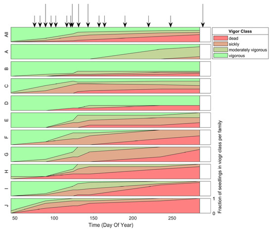
Figure 1.
Fraction of seedlings (y-axis) in each vigor class based on visual assessments of inoculated seedlings over time (x-axis) for all infected seedlings (top panel) and per family (A-J panels). Note the differences per family in terms of the fraction of seedlings within each vigor class and the timing of vigor reduction. Arrows indicate the hyperspectral image acquisition dates. The longer arrows indicate the image acquisition dates that were closest to a visual assessment and were therefore used for vigor classification. Hyperspectral imaging (HSI) was more frequent during the onset of the disease. Once the change in symptom expression slowed down the frequency of HSI was reduced as well.
3.2. Classification Results
3.2.1. White Pine Blister Rust Infection Identification Detected by Hyperspectral Imaging
Identification of infection using hyperspectral imaging (HSI) was successful over the entire duration of the experiment with an average accuracy of 87% (κ = 0.75) (Figure 2). There was a time dependency on the accuracy of HSI, increasing from 80% at the start of the experiment to 90% mid-season. The improvement in classification accuracy coincided with the increase in seedling symptom expression in the visual vigor inspection. Surprisingly, the accuracy of HSI decreased after this peak even though the percentage of seedlings exhibiting visible symptoms continued to increase. To assess how effective HSI was at finding infected seedlings before they have visual symptoms (beyond needle spots) we compared the probability that an infection was detected using HSI to the percentage of impacted seedlings that were in vigor class two or higher (Figure 3). HSI was able to detect 86% of the infected seedlings on average. Even at the beginning of the experiment, HSI detected over 80% of the infected seedlings when only 20% of the infected seedlings were impacted in terms of vigor. For the duration of the experiment, 20% of the seedlings remained vigorous. These vigorous, but infected, seedlings were responsible for 71% of the error in HSI infection detection. Thus, HSI only missed 4% of infected seedlings that were impacted in terms of vigor according to the expert’s assessments (29% of the 14% error).

Figure 2.
Classification accuracy distribution over time using hyperspectral imaging for identifying infected and non-inoculated control seedlings using a 10-fold cross-validation, repeated 19 times. Note that there was a time dependency on the accuracy of HSI, increasing from 80% at the start of the experiment to 90% mid-season.
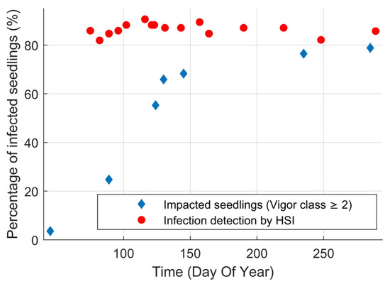
Figure 3.
Percentage of infected seedlings over time whose vigor was impacted by the rust (vigor class ≥2) and percentage of infected seedlings that were identified as being infected by hyperspectral imaging (averaged). Note that at the start of the experiment, HSI was able to successfully identify 80% of the inoculated seedlings when only 20% were vigor-impacted.
3.2.2. Classification Accuracy of Infection per Family
The families were selected to span a wide range in geographic and climatic distribution, which may include individuals with genetic resistance to white pine blister rust. Therefore, we examined whether families would influence the ability of our approach to identifying infected from non-inoculated control seedlings. Inaccuracy among families varied by a factor of eight from 3.9% to over 30% (Figure 4). False negatives were on average 1.2% for the five families where diseased seedlings were most easily identified. However, the three families with the highest percent of vigorous seedlings, families A, B, and D, had a 16% false-negative rate for disease classification (Figure 4). There was a strong correlation between mortality rate and classification accuracy, R2 was 0.51 (Figure 5a). Family C had a high classification accuracy and low false-negative rate even though its mortality rate was low. However, even though mortality rates were low, the seedlings did exhibit a phenotypic impact from the rust (Figure 1). The correlation between the rate of vigorous seedlings and classification accuracy per family was 0.67 (Figure 5b). These results mirrored family susceptibility, with 71% of false-negatives occurring in vigorous seedlings. Thus, for families that see a reduction in vigor status, accuracy in classifying diseased from control plants was remarkably high, up to 96%. Strikingly, even in the cases of genetically resistant families (low mortality rates), over two-thirds of infected trees were classified properly.
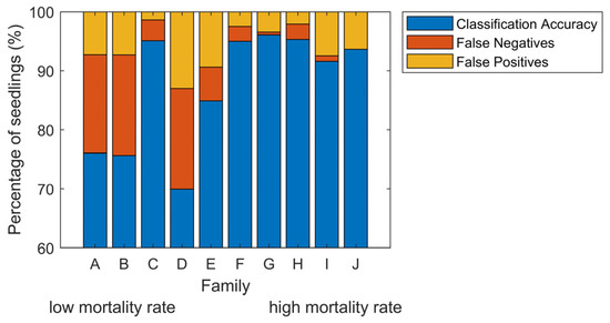
Figure 4.
Mean classification results over 16 dates per family. The error (100%—Classification Accuracy) per family is explained in terms of false-negatives and false-positives. Families are ordered based on the mortality rate at the end of the experiment, the same as in Figure 1.

Figure 5.
Correlation for (a) mortality rate and classification accuracy, and (b) vigorous rate and classification accuracy. Each data point represents a family indicated with the letter label.
3.2.3. Classification into Vigor Class
The average classification accuracy over the five dates for the vigor class was 74.2% (κ = 0.62). Because the grouping was unbalanced, i.e., half of the seedlings were non-inoculated control seedlings and the other half was divided into four vigor classes, we used the confusion matrix to thoroughly assess the precision and probability of detection (Table 1).

Table 1.
Confusion matrix for vigor groupings classification between TRUE classes (from visual assessments) and PREDICTED classes (from hyperspectral imaging model) averaged over five dates, 0 = non-inoculated control seedlings, 1 = infected & vigorous, 2 = infected and moderately vigorous, 3 = infected and sickly, 4 = infected and dead. Probability of detection is the number of correct labels divided by the total number of observed seedlings in that class; precision is the number of correct labels divided by the total predicted seedlings in that class; AUC is the average area under the curve for a receiver operating characteristic curve for that class versus the rest; OA is the overall accuracy, and; κ is the kappa coefficient. The table points out that seedlings in vigor-class 2 were difficult to separate from classes 1 and 3.
For the seedlings that were predicted by the model to be in class 2, only 37.1% were visually identified as class 2. Most seedlings predicted to be in class 2 were truly in classes 3 or 1. Class 2 also had a low probability of detection (35.1%), meaning that the model was not able to find the majority of the class 2 seedlings. Seedlings that truly fall in class 2 might not have a strong enough signal to be distinguished from seedlings in class 3 or 1 (see Figure S3 for spectral signatures of each class). Whereas the precision and probability of detection for class 2 were the lowest, the AUC was the lowest for class 1. This implies that for this particular case, class 2 was the most difficult class to accurately identify. However, class 1 is the most difficult one in general, when this classifier is applied to another population.
Owing to the difficulty in separating classes 2 and 3 and the subjectivity in visual scoring, we re-applied the classification with classes 2 and 3 merged. The overall accuracy increased by 5.5 percentage points to 79.7% (Table 2). The precision of every class was 58.1% or higher, an improvement from 37.1% found with all five classes considered. The AUCs for classes 0, 1, and 4 remained at the same level as for the previous case, where the AUC for the merged 2 and 3 class increased compared to the separate classes. The relatively low AUC value for class 1 (0.792) showed that this class is still the hardest to distinguish. The precision and AUC-values are now closely correlated (R2 was 0.90 when merging classes 2 and 3 vs 0.53 for the original case without merging). The probability of detecting seedlings in vigor class 1 remained relatively low, 59.1% (Table 2). However, 29% of the imaged seedlings in vigor class 1 were still developing symptoms. These infected seedlings were vigorous (vigor class 1) and were in vigor class 2 or higher at the next visual assessment. Out of the 46 pre-affected seedlings in terms of vigor, 44 were detected by the trained classifier as infected even though their vigor had not yet been compromised.
Table 2.
Confusion matrix with class 2 and 3 merged for vigor groupings classification between TRUE classes (from visual assessments) and PREDICTED classes (from hyperspectral imaging model) averaged over 5 dates. 0 = non-inoculated control seedlings, 1 = infected and vigorous, 2 = infected and moderately vigorous, 3 = infected and sickly, 4 = infected and dead. Probability of detection is the number of correct labels divided by the total number of observed seedlings in that class; precision is the number of correct labels divided by the total predicted seedlings in that class; AUC is the average area under the curve for a receiver operating characteristic curve for that class versus the rest; OA is the overall accuracy, and; κ is the kappa coefficient. Note that OA improved by 5.5 percentage points compared to the results in Table 1.
3.3. Hyperspectral Feature Importance
We have shown that hyperspectral imaging was able to detect infection. Next, we address which parts of the spectrum and which hyperspectral features contributed most to the successful classification. We aimed to gain more insight into which biological and chemical processes in the seedlings might have been impacted by blister rust infection, and the timing of these impacts.
3.3.1. Feature Identification for Infection Detection
The strength of each band in the spectrum to separate the mean of the two classes, inoculated and control seedlings, was assessed using the p-value resulting from a 2-sample t-test. For all dates, the spectra between 600 and 700 nm had the smallest p-value (<2 × 10⁻⁵) (Figure 6a). Over time, this 600–700 region became more significant as the disease progressed. This region also became visible to the naked eye because there was browning. The same region and trend were identified using the Bhattacharyya distance (BD) (Figure 6b).
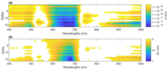
Figure 6.
(a) p-value of 2-sample t-test to assess the relative importance among wavelengths to distinguish inoculated from control seedlings over time. Cooler colors represent smaller p-values. In white are non-significant wavelengths (p > 0.05). (b) Bhattacharyya distances of wavelengths over time between distributions of reflectance for inoculated and control seedlings. This is an indicator of how successful a wavelength is at separating infected from control seedlings (1 is successful and 0 is unsuccessful). In white are BD-values < 0.05.
VIs can be used to derive physiological and biogeochemical properties of vegetation, but which one is best able to find infection? The highest classification accuracy was reached using indices sensitive to the xanthophyll cycle, PRI570, PRI, and PRIn (Figure 7). The log-transformed p-value and classification accuracy were highly correlated, Pearson’s R2 = 0.82. However, if we ranked p-values, we would miss the VI with the best classification accuracy, PRIn. For the Bhattacharyya distance (BD-value), the highest value was for the VI with the highest classification accuracy. However, PRI570, with the third-highest classification accuracy, was ranked 7th based on the BD-value. Moreover, there was an outlier, the modified normalized difference index (mND) was 9th in BD-rank, with a low classification accuracy of around 50% and therefore no predictive power. However, this VI did have a non-significant p-value of 0.36 and would thus never be identified by this metric. This suggests that a combined p-value and BD-value approach, here referred to as the ‘new search algorithm’, would be beneficial.
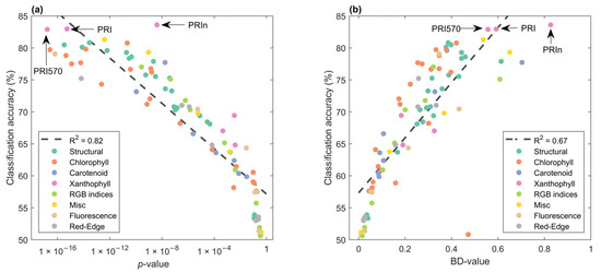
Figure 7.
Mean classification accuracy over 16 dates (y-axis) and mean variable on the x-axis. (a) p-values from a 2-sample t-test (H0 = means for treatments were the same). Noteworthy indices with the highest classification accuracy are indicated with arrows. Spearman’s rho for the first n identified VIs using the ‘new search algorithm’ was −0.54. Colors were used for VI groupings. (b) Bhattacharyya distances vs classification accuracy per VI, Spearman’s rho for the first n identified VIs using the ‘new search algorithm’ was 0.43.
3.3.2. Feature Identification Using ‘New Search Algorithm’
Here we present the results of using both BD and p-value to identify the most informative VI. This is validated against the classification accuracy of each VI. Using the new search algorithm, we ranked the VIs. We report on Spearman’s ranked rho and whether the best VI has been ranked first.
The new search algorithm was more successful than either p-value ranking or BD-value ranking in both identifying the VIs with the highest accuracies first as well as the overall ranking of the VIs. The new search algorithm was able to rank the two VIs with the highest classification accuracies first (PRI570 and PRIn, Figure 8). In comparison, PRIn would have been ranked 31st using solely the p-value. Spearman’s rho for the ranked test was −0.75 on the identified VIs. This was a stronger relationship than Spearman’s rho for the same number of identified VIs (here n = 36) for either p-value ranking (rho = −0.54) and BD-ranking (rho = 0.43). Note that these single VIs reach an average classification accuracy of 83%, only 4 percentage points lower than the 87% for full spectrum classification.
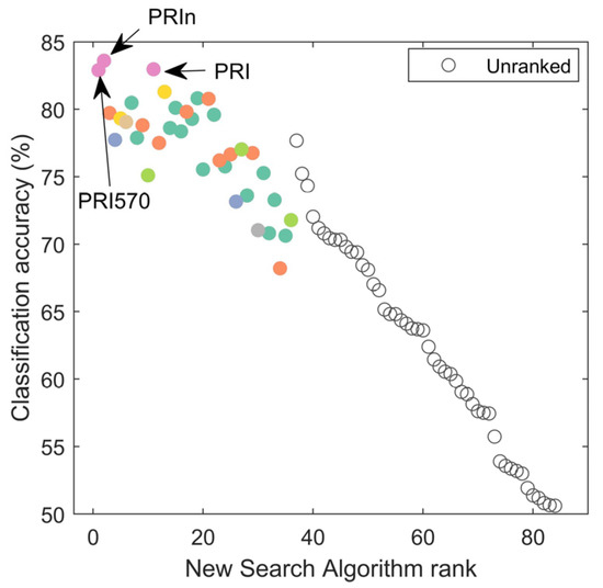
Figure 8.
Identified VIs (ranked on the x-axis) based on the new search algorithm for most informative VI. Spearman’s rank test rho is −0.75. Unranked VIs did not meet the minimum criteria of BDi > median (BD) and pi < median(p). Colors were used for VI groupings and are the same as in Figure 7. Noteworthy indices are indicated with arrows and labels; these indices had the highest classification accuracies.
The VI determined to be most suitable was found to be time-dependent. The best VIs during early assessments (the first four dates of data acquisition) were the xanthophyll indices (Figure 9). Interestingly, PRIn had a p-value that ranked 33rd out of 84 (not shown here), but it did have the highest classification accuracy. Because of its high BD-value, PRIn was identified second by the new search algorithm. For the late assessment (the last four dates of data acquisition), the xanthophyll indices were no longer the best, and there was a shift to the structural and carotenoid indices. The new search algorithm was able to identify the VIs with the highest classification accuracies of around 84%, the plant senescencing reflectance index (PSRI) and greenness index (GI). The PSRI is a carotenoid index, and the GI is a structural index.

Figure 9.
Early time and late time assessment of ranked search algorithm. (a) “Early time” was averaged over the first four acquisition dates when the number of infected seedlings with symptoms <32%. (b) “Late time” was averaged over the last four acquisition dates when the number of infected seedlings with symptoms >72%. Noteworthy indices with the highest classification accuracy are indicated with arrows and labels. Colors were used for VI groupings and are the same as in Figure 7.
3.3.3. New Search Algorithm Applied to All Features
The new search algorithm was tested and evaluated on the 84 VIs. Here we applied the method to the entire hyperspectral feature set to identify more regions of interest. Because there are around 150,000 features in this analysis, the results discussed here will be limited to the first 6 identified features (Table 3). For all time segments (overall, early, and late time) the first ranked features were simple ratios. In second place came the VIs that were identified before (xanthophyll cycle VIs for overall and early, and the senescence VI for late time). This strengthened the positions of these VIs. For overall and early time segments, most of the identified features were similar, with simple ratios between 575 nm (+/−10) and 525 nm (+/−6). For the late time segment, there was a shift to the simple ratios between 680 nm (+/−10) and 520 nm (+/−10).
Table 3.
Identified features using the new search algorithm for overall (average), early time (first four acquisition dates), and late time (last four acquisition dates) for the entire hyperspectral feature set (~150,000 variables). Note that the second identified feature for each of the time segments is a VI. This strengthened the positions of these VIs.
3.3.4. Feature Identification for Family Separation
The most informative wavelengths for family discrimination were between 500 and 700 nm within non-inoculated control seedlings (Figure S4). The smallest p-value was found for 542 nm (average p-value over time is 1.6 × 10⁻²). For inoculated seedlings, the same range of wavelengths was most significant (Figure S5). However, the range of wavelengths that had a significant p-value and magnitude of significance per wavelength was larger. Therefore, the same wavelengths were of interest, but for the inoculated seedlings these wavelengths showed more difference than for the control group. Within both groups of seedlings (in inoculated and in control), MCARI (Modified Chlorophyll Absorption Ratio Index) was found most significant for separation between families with an average p-value < 1 × 10⁻⁸. Even after taking away the timing differences in symptom expression, by combining all dates, the best separator was still MCARI for infected seedlings, however, we cannot compare the p-values due to size-effect. Note that no Bhattacharyya distance can be calculated for multiple class distributions.
3.3.5. Feature Identification for Vigor Classes
The wavelengths between 600 and 700 nm had the greatest significance (Figure S6). This was the same range that was found significant for infection detection. As to which hyperspectral feature was most informative, on average, PRIn showed the strongest power of separation for vigor classes. For all dates combined, we analyzed the distribution of PRIn per class (Figure 10). Looking at the probability density function of each class, generated with a multinomial regression, we observed a strong separation between classes, except for class 2. This was similar to the results of the vigor classification observed in the confusion matrix (Table 1) when using the entire spectrum. Furthermore, there was a separation apparent in inoculated seedlings between unaffected (seedlings remaining in vigor 1 class for the duration of the experiment) and pre-affected (seedlings in vigor 1 class at the date of the hyperspectral data acquisition, but in class 2 or higher during the next assessment) (2-sample t-test p = 1.97 × 10⁻¹⁴).
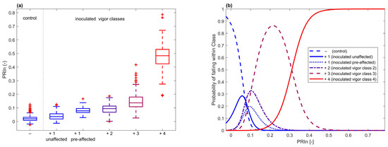
Figure 10.
(a) PRIn distribution for all dates combined for ‘−’ non-inoculated control seedlings, ‘+1 unaffected’ infected seedlings that remained unaffected in terms of vigor for the duration of the experiment, ‘+1 pre-affected’ infected seedlings that were not affected in terms of vigor on the date that PRIn was calculated but were affected during the next visual assessment, ‘+2’, ‘+3’, and ‘+4’ infected seedlings in vigor classes 2, 3, and 4, respectively. (b) Multinomial regression for probabilistic classification using PRIn, showing the ability of this single VI to separate seedlings for vigor classes.
4. Discussion
We have demonstrated that a hyperspectral imaging platform in combination with data-driven machine learning was able to identify stages of infection. Computing VIs suggested by others may give us insight into which biological and chemical processes in the seedlings were affected.
Classification accuracy for infection varied per family. It was expected that the families had different levels of resistance to the disease. Seedlings that were not impacted would therefore be inseparable from control seedlings. This was apparent in the 71% rate of false-negatives that were caused by seedlings that were infected but not impacted by the disease in terms of vigor. Another study similarly found that there were no significant differences in spectral signatures between infected and control seedlings in resistant barley families [7].
The new search algorithm was able to identify the best features for all three time-windows, overall, early, and late. This easy-to-implement method provides the scientific community with a tool to quickly identify informative hyperspectral features for the separation of classes without having to go through the time-consuming process of machine learning classification. This can be used in data-driven approaches where we reduce the subjectivity in feature design. Note that one could also use a linear SVM to get the weights of the features in the learner, however, this would be considered a feature forward selection and finds features that have a low correlation but do explain the pattern in the data. To assess which processes in the plant are affected, we were interested in the absolute value of separation, no matter if features were highly correlated. Thus, the weights of the linear SVM cannot be used in this matter.
For each separation task (i.e., infection and vigor class) the same region of the spectrum was of interest. The 600–700 nm region was found to have the strongest power of separation. These wavelengths are associated with chlorophyll reflectance [42]. Vegetation with a higher content of chlorophyll is better able to absorb and use red light for photosynthesis. In the pathogen-impacted seedlings, a relatively higher amount of light in this spectral region was reflected which implies that the photosynthetic capacity in the seedlings was reduced.
This reduced photosynthetic capacity was corroborated by the identification of informative VIs. Using our new search algorithm, we identified that the largest power of separation for infection detection (plus pre-affected), as well as for vigor classes, was for different forms of the photochemical reflectance, or xanthophyll, indices. For infection detection, PRI570 and PRIn were most informative. PRI570 is a normalized difference index for 570 and 531 nm developed for tracking photosynthetic efficiency [43]. It is sensitive to the epoxidation status of the xanthophyll-cycle pigments. In practice, it is often found to be correlated to water stress indicators such as stomatal conductance [44,45,46]. PRIn [44] is a variant of PRI, where PRI570 is normalized by the renormalized difference vegetation index, RDVI. PRIn was found to be sensitive to water stress. This could mean that the spectral signal in the diseased seedlings might actually be an indicator of water stress. Further research is needed to determine whether there is a difference in reflectance between biotic white pine blister rust infection and abiotic water stress.
PRIn is calculated with five bands, ranging from 531 to 800 nm. It would be possible to measure this number of bands with a less expensive and more data-parsimonious multispectral camera. However, multispectral cameras often measure reflectance in broader bands in contrast to the narrow bands of hyperspectral cameras, and the crispness of band definition would be important. We trained an SVM classifier with only the narrowband PRIn. This resulted in an overall accuracy of 71.4%, κ = 0.55, and for classes 2 and 3 merged, the overall accuracy was 75.5%, κ = 0.61. For a broadband approach, the average reflectance in the 10 nm window around the center wavelength was used to calculate the multispectral equivalent PRIn. The classification accuracy for all classes was 69.3%, κ = 0.52 and for classes 2 and 3 merged, the overall accuracy was 73.6%, κ = 0.58. Thus, we found only 5 to 6.6% lower accuracy than classification with the full narrowband spectrum.
For advanced infection (late time), the plant senescence reflectance index, PSRI [47] was the most successful VI. This index is sensitive to the carotenoids-chlorophyll ratio and is used to track, as the name implies, the senescence of a plant. It is calculated with three bands: 680, 500, and 750 nm, and it is sensitive to changes in the ratio between carotenoid and chlorophyll pigments.
Differences in reflectance between families for control seedlings were also observed (Figure S7). Control seedlings from family A showed higher reflectance in the 700–1000 nm region than the other families. Reflectance in the NIR is caused by spongy mesophyll structure and is an indicator of biomass depth of the canopy [48]. Family A has a significantly bigger and thicker canopy than the other families (see Figure S8 for an example). A similar correlation between canopy area, closely related to canopy thickness, was also visible in control seedlings in family H. This family had the lowest median canopy area and had a slightly lower reflectance in the NIR than the others. For discriminating control seedlings based on the family, the best range in the spectrum was between 500 and 700 nm, with a peak at 542 nm. This wavelength is associated with chlorophyll content [49].
The difference between families was even more visible in the inoculated seedlings because the families had different levels of resistance and susceptibility (Figure S9). This might not be just a difference in reaction to the pathogen but could additionally be a difference in timing in its progression. A delay in symptom-expression suggests a type of quantitative disease resistance to white pine blister rust. MCARI was found most significant from the VI-list to separate family groupings. MCARI is an index that uses 3 bands, 712, 682, and 539 nm, and was developed to be sensitive to chlorophyll content. This implies that the difference in genotypes is driven by a difference in chlorophyll content [50]. This was true for both inoculated and control seedlings. Similarly, Wang et al. [51] found MCARI significant to distinct genotypes of rice.
With these observed differences between families, there might be a potential for automatic family and white pine blister rust detection. Preliminary results showed a classification accuracy of 28.5% (κ = 0.18) for classifying only inoculated seedlings into family groupings. For control seedlings, this was 38.4% (κ = 0.28). Moreover, to separate for family and treatment (20 classes) the classification accuracy is 27% (κ = 0.22) (Tables S3–S5). To further explore the potential of automatic family identification, an experiment focused on family and infection detection needs to be designed and conducted.
5. Conclusions
We have assessed the potential of using hyperspectral imaging to track the progression and severity of white pine blister rust infection in southwestern white pine seedlings and to validate the new search algorithm for simplified feature identification. The hyperspectral imaging platform was able to detect infection with an 87% accuracy over the entire duration of the experiment. HSI only missed 4% of infected seedlings that were impacted in terms of vigor according to the expert’s assessments. The classification accuracy for infection detection per family varied from 69.9 to 96.1%. Families that have a high mortality rate have a high classification accuracy and vice versa. In resistance trials, it is important to be able to track the severity of the infection. Here, we found a 79.7% classification accuracy for the vigor class, and the higher temporal rate of screening allowed us to identify the delayed impact of the disease in some families. Multinomial regression was applied to generate a probabilistic classifier using PRIn. This VI, calculated using five bands, was able to classify for vigor class with a 75.5% accuracy, showing the potential of a specially tuned multi-spectral camera.
We proposed a new search algorithm to identify hyperspectral features of interest. This method ranked the xanthophyll indices PRIn and PRI570 first for infection detection among all 84 VIs. These VIs were also found most useful in classifying seedlings for infection (83% classification accuracy). These indices are related to the photosynthetic health of vegetation. At the family level, there were significant differences in the 500 to 700 nm range and for the MCARI index, suggesting a difference in chlorophyll content.
The new search algorithm successfully ranked the features based on their p-value and Bhattacharyya distance and was able to identify the VIs with the highest classification accuracy. The absolute ranking-parameter, Spearman’s rho, for the new search algorithm was 0.75, compared to 0.54 for p-value and 0.43 for BD. We expect that this algorithm can be applied to other data sets and further help the scientific community. One closely related application is the field of high-throughput phenotyping. Moreover, this method could be used to select wavelengths to create a less expensive and more data-parsimonious multispectral camera.
Supplementary Materials
The following are available online at https://www.mdpi.com/2072-4292/12/24/4041/s1, Table S1. Overview of the number of seedlings within each family per treatment (inoculated and control), the geographic origin of families, and the Köppen climate classification. Figure S1. Photo of the experiment setup. In the bottom of the picture are the pots with the seedlings, and at the top is the hyperspectral camera on the hyper-rail. Table S2. List of VIs used in this study. Figure S2. Schematic of the ‘New search algorithm’ for feature importance. Figure S3. Spectral plots of (a) average reflectance per vigor class plus control seedlings and (b) mean normalized difference using mean spectrum of control seedlings (normalized difference = (reflectance vigor class x − reflectance control)/(reflectance vigor class x + reflectance control). Figure S4. p-values for a one-way ANOVA to assess the significance of differences in mean reflectance families in non-inoculated control seedlings per wavelength over time. This is an indicator of how successful a wavelength is at separating seedlings for family. In white are non-significant bands (p > 0.05). Figure S5. p-values for a one-way ANOVA to assess the significance of differences in mean reflectance between families in inoculated seedlings per wavelength over time. This is an indicator of how successful a wavelength is at separating inoculated seedlings for family. In white are non-significant bands (p > 0.05). Figure S6. p-values for a one-way ANOVA to assess the significance of differences in mean reflectance between severity classes (0 through 4) per wavelength over time. This is an indicator of how successful a wavelength is at separating for symptom severity class. In white are non-significant bands (p > 0.05). Figure S7. Mean reflectance of non-inoculated control seedlings per family (A–J) for DOY 75, DOY 190, and DOY 289. Figure S8. Examples of seedlings over time for inoculated and non-inoculated control seedlings for three families. (a) J, (b) C, and (c) A. These are RGB composites and it shows the vegetation mask that was used to extract pixels. Family J (top panel) is a highly susceptible family, in contrast to family A (bottom panel) that showed few symptoms. Moreover, the differences between the families’ control seedlings were apparent in size and coloring. Figure S9. Mean reflectance of inoculated seedlings per family (A–J) over time. Table S3. Confusion matrix for inoculated seedlings classified for family grouping. Table S4. Confusion matrix for non-inoculated control seedlings for family grouping. Table S5. Confusion matrix for family and treatment (inoculated and control) grouping.
Author Contributions
Conceptualization, M.H., G.F.M.P., J.S.J., and J.S.S.; Methodology, M.H., G.F.M.P., J.S.J., J.S.S., and R.A.S.; Software, M.H.; Validation, M.H.; Formal Analysis, M.H.; Investigation, M.H., G.F.M.P., and J.S.J.; Resources, J.S.J., R.A.S., K.M.W., C.S., and J.S.S.; Data Curation, M.H., G.F.M.P., and J.S.J.; Writing—Original Draft Preparation, M.H.; Writing—Review & Editing, M.H., G.F.M.P., J.S.J., C.S., K.M.W., R.A.S., and J.S.S.; Visualization, M.H.; Supervision, M.H., G.F.M.P., J.S.J., J.S.S., R.A.S., and C.S.; Project Administration, M.H., G.F.M.P., J.S.J., and C.S.; Funding Acquisition, J.S.S., C.S., K.M.W., and R.A.S. All authors have read and agreed to the published version of the manuscript.
Funding
This work is supported by the National Science Foundation under grant nr. NSF-EAR 1440506, NSF-DEB 1442456-1442597, and NSF-CCF 1521687 (Collaborative Research: Facility Support: Center for Transformative Environmental Monitoring Programs (CTEMPs); Collaborative Research: Blending Ecology and Evolution using Emerging Technologies to Determine Species Distributions with a Non-native Pathogen in a Changing Climate, and Collaborative Research; CompSustNet: Expanding the Horizons of Computational Sustainability, respectively).
Acknowledgments
We would like to thank the volunteers in the greenhouse (Manuel Lopez, Adam Sibley, and Elizabeth Jachens), the OSU greenhouse staff, and the Dorena staff who did the spore collection and inoculations. We appreciate the tree climbing field crews, graduate students, and lab technicians at Northern Arizona University, for collecting and processing seed. Finally, we would like to thank the editor and reviewers for their valuable input.
Conflicts of Interest
The authors declare no conflict of interest.
References
- Parmesan, C.; Yohe, G. A globally coherent fingerprint of climate change impacts across natural systems. Nature 2003, 421, 37–42. [Google Scholar] [CrossRef] [PubMed]
- Trumbore, S.; Brando, P.; Hartmann, H. Forest health and global change. Science 2015, 349, 814–818. [Google Scholar] [CrossRef] [PubMed]
- Shirk, A.J.; Cushman, S.A.; Waring, K.M.; Wehenkel, C.A.; Leal-Sáenz, A.; Toney, C.; Lopez-Sanchez, C.A. Southwestern white pine (Pinus strobiformis) species distribution models project a large range shift and contraction due to regional climatic changes. For. Ecol. Manag. 2018, 411, 176–186. [Google Scholar] [CrossRef]
- Chakraborty, S.; Tiedemann, A.V.; Teng, P.S. Climate change: Potential impact on plant diseases. Environ. Pollut. 2000, 108, 317–326. [Google Scholar] [CrossRef]
- National Academies of Sciences and Medicine. Forest Health and Biotechnology: Possibilities and Considerations; National Academies Press: Washington, DC, USA, 2019; ISBN 978-0-309-48288-2. [Google Scholar]
- Fei, S.; Morin, R.S.; Oswalt, C.M.; Liebhold, A.M. Biomass losses resulting from insect and disease invasions in US forests. Proc. Natl. Acad. Sci. USA 2019, 116, 17371–17376. [Google Scholar] [CrossRef] [PubMed]
- Kuska, M.; Wahabzada, M.; Leucker, M.; Dehne, H.-W.; Kersting, K.; Oerke, E.-C.; Steiner, U.; Mahlein, A.-K. Hyperspectral phenotyping on the microscopic scale: Towards automated characterization of plant-pathogen interactions. Plant Methods 2015, 11, 28. [Google Scholar] [CrossRef]
- Sniezko, R.A.; Koch, J. Breeding trees resistant to insects and diseases: Putting theory into application. Biol. Invasions 2017, 19, 3377–3400. [Google Scholar] [CrossRef]
- Sniezko, R.A.; Johnson, J.S.; Savin, D.P. Assessing the durability, stability, and usability of genetic resistance to a non-native fungal pathogen in two pine species. Plants People Planet 2020, 2, 57–68. [Google Scholar] [CrossRef]
- Showalter, D.N.; Raffa, K.F.; Sniezko, R.A.; Herms, D.A.; Liebhold, A.M.; Smith, J.A.; Bonello, P. Strategic development of tree resistance against forest pathogen and insect invasions in defense-free space. Front. Ecol. Evol. 2018, 6, 124. [Google Scholar] [CrossRef]
- Sniezko, R.A. Resistance breeding against nonnative pathogens in forest trees - Current successes in North America. Can. J. Plant Pathol. 2006, 28, S270–S279. [Google Scholar] [CrossRef]
- Kumar, A.; Lee, W.S.; Ehsani, R.J.; Albrigo, L.G.; Yang, C.; Mangan, R.L. Citrus greening disease detection using aerial hyperspectral and multispectral imaging techniques. J. Appl. Remote Sens. 2012, 6, 063542. [Google Scholar] [CrossRef]
- Devadas, R.; Lamb, D.W.; Simpfendorfer, S.; Backhouse, D. Evaluating ten spectral vegetation indices for identifying rust infection in individual wheat leaves. Precis. Agric. 2009, 10, 459–470. [Google Scholar] [CrossRef]
- López-López, M.; Calderón, R.; González-Dugo, V.; Zarco-Tejada, P.J.; Fereres, E. Early detection and quantification of almond red leaf blotch using high-resolution hyperspectral and thermal imagery. Remote Sens. 2016, 8, 276. [Google Scholar] [CrossRef]
- Calderón, R.; Navas-Cortés, J.A.; Lucena, C.; Zarco-Tejada, P.J. High-resolution airborne hyperspectral and thermal imagery for early detection of Verticillium wilt of olive using fluorescence, temperature and narrow-band. Remote Sens. Environ. 2013, 139, 231–245. [Google Scholar] [CrossRef]
- Calderón, R.; Navas-Cortés, J.A.; Zarco-Tejada, P.J. Early detection and quantification of Verticillium wilt in olive using hyperspectral and thermal imagery over large areas. Remote Sens. 2015, 7, 5584–5610. [Google Scholar] [CrossRef]
- Rumpf, T.; Mahlein, A.-K.; Steiner, U.; Oerke, E.-C.; Dehne, H.-W.; Plümer, L. Early detection and classification of plant diseases with support vector machines based on hyperspectral reflectance. Comput. Electron. Agric. 2010, 74, 91–99. [Google Scholar] [CrossRef]
- Mahlein, A.-K.; Steiner, U.; Dehne, H.-W.; Oerke, E.-C. Spectral signatures of sugar beet leaves for the detection and differentiation of diseases. Precis. Agric. 2010, 11, 413–431. [Google Scholar] [CrossRef]
- Gold, K.M.; Townsend, P.A.; Chlus, A.; Herrmann, I.; Couture, J.J.; Larson, E.R.; Gevens, A.J. Hyperspectral Measurements Enable Pre-Symptomatic Detection and Differentiation of Contrasting Physiological Effects of Late Blight and Early Blight in Potato. Remote Sens. 2020, 12, 286. [Google Scholar] [CrossRef]
- Leucker, M.; Wahabzada, M.; Kersting, K.; Peter, M.; Beyer, W.; Steiner, U.; Mahlein, A.-K.; Oerke, E.-C. Hyperspectral imaging reveals the effect of sugar beet QTLs on Cercospora leaf spot resistance. Funct. Plant Biol. 2017, 44, 1–9. [Google Scholar] [CrossRef]
- Alisaac, E.; Behmann, J.; Kuska, M.T.; Dehne, H.-W.; Mahlein, A.-K. Hyperspectral quantification of wheat resistance to Fusarium head blight: Comparison of two Fusarium species. Eur. J. Plant Pathol. 2018, 152, 869–884. [Google Scholar] [CrossRef]
- Lausch, A.; Erasmi, S.; King, D.J.; Magdon, P.; Heurich, M. Understanding forest health with Remote sensing-Part II-A review of approaches and data models. Remote Sens. 2017, 9, 129. [Google Scholar] [CrossRef]
- Conklin, D.A.; Fairweather, M.L.; Ryerson, D.E.; Geils, B.W.; Vogler, D.R. White pines, blister rust, and management in the Southwest. USDA For. Serv. Southwest Reg. R3-Fh-09-01 2009, 16, 3. [Google Scholar]
- Sniezko, R.A.; Mahalovich, M.F.; Schoettle, A.W.; Vogler, D.R. Past and current investigations of the genetic resistance to Cronartium ribicola in high-elevation five-needle pines. In The Future of High-Elevation, Five-Needle White Pines in Western North America. Proc High Five Symp RMRS-P-63; Keane, R.E., Tomback, D.F., Murray, M.P., Smith, C.M., Eds.; USDA Forest Service Rocky Mountain research Station: Fort Collins, CO, USA, 2011; pp. 246–264. [Google Scholar]
- King, J.N.; David, A.; Noshad, D.; Smith, J. A review of genetic approaches to the management of blister rust in white pines. For. Pathol. 2010, 40, 292–313. [Google Scholar] [CrossRef]
- Kinloch, B.B. Forest Pathology for the Last Century: A Retrospective and Directions for the Future White Pine Blister Rust in North America: Past and Prognosis. Phytopathology 2003, 93, 1044–1047. [Google Scholar] [CrossRef] [PubMed]
- Looney, C.E.; Waring, K.M. Patterns of forest structure, competition and regeneration in southwestern white pine (Pinus strobiformis) forests. For. Ecol. Manag. 2012, 286, 159–170. [Google Scholar] [CrossRef]
- Hoff, R.; Bingham, R.T.; McDonald, G.I. Relative blister rust resistance of white pines. Eur. J. For. Pathol. 1980, 10, 307–316. [Google Scholar] [CrossRef]
- Wyka, S.A.; Munck, I.A.; Brazee, N.J.; Broders, K.D. Response of eastern white pine and associated foliar, blister rust, canker and root rot pathogens to climate change. For. Ecol. Manag. 2018, 423, 18–26. [Google Scholar] [CrossRef]
- Kegley, A.J.; Sniezko, R.A. Variation in blister rust resistance among 226 Pinus monticola and 217 P. lambertiana seedling families in the Pacific Northwest. In Breeding and Genetic Resources of Five-Needle Pines: Growth, Adaptability and Pest Resistance; Sniezko, R.A., Samman, S., Schlarbaum, S.E., Kriebel, H.B., Eds.; USDA Forest Service, Rocky Mountain Research Station RMPS-P-32: Fort Collins, CO, USA, 1998; pp. 209–225. [Google Scholar]
- Sniezko, R.A.; Kegley, A.J.; Danchok, R. White pine blister rust resistance in North American, Asian and European species-results from artificial inoculartion trials in Oregon. Ann. For. Res. 2008, 51, 53–66. [Google Scholar]
- Lopez Alcala, J.M.; Haagsma, M.; Udell, C.J.; Selker, J.S. HyperRail: Modular, 3D Printed, 1-100 meter, Programmable, and Low-cost Linear Motion Control System for Imaging and Sensor Suites. HardwareX 2019, 6, e00081. [Google Scholar] [CrossRef]
- Smith, G.M.; Milton, E.J. The use of the empirical line method to calibrate remotely sensed data to reflectance. Int. J. Remote Sens. 1999, 20, 2653–2662. [Google Scholar] [CrossRef]
- Thenkabail, P.P.S.; Smith, R.B.; Pauw, E. De Hyperspectral vegetation indices and their relationships with agricultural crop characteristics. Remote Sens. Environ. 2000, 71, 158–182. [Google Scholar] [CrossRef]
- Serrano, L.; Peñuelas, J.; Ustin, S.L. Remote sensing of nitrogen and lignin in Mediterranean vegetation from AVIRIS data: Decomposing biochemical from structural signals. Remote Sens. Environ. 2002, 81, 355–364. [Google Scholar] [CrossRef]
- Carter, G.A. Ratios of leaf reflectances in narrow wavebands as indicators of plant stress. Remote Sens. 1994, 15, 697–703. [Google Scholar] [CrossRef]
- Dixit, L.; Ram, S. Quantitative analysis by derivative electronic spectroscopy. Appl. Spectrosc. Rev. 1985, 21, 311–418. [Google Scholar] [CrossRef]
- Cohen, J. A Coefficient of Agreement for Nominal Scales. Educ. Psychol. Meas. 1960, 20, 37–46. [Google Scholar] [CrossRef]
- Bradley, A.E. The use of the area under the ROC curve in the evaluation of machine learning algorithms. Pattern Recognit. 1997, 30, 1145–1159. [Google Scholar] [CrossRef]
- Bhattacharyya, A. On a measure of divergence between two statistical populations defined by their probability distributions. Bull. Calcutta Math. Soc. 1943, 35, 99–109. [Google Scholar]
- Haagsma, M.; Page, G.F.M.; Johnson, J.S. Hyperspectral Imagery of Pinus Strobiformis Infected with Fungal Pathogen, Version 1; Oregon State University: Corvallis, OR, USA, 2020. [Google Scholar] [CrossRef]
- Chappelle, E.W.; Kim, M.S.; McMurtrey III, J.E. Ratio analysis of reflectance spectra (RARS): An algorithm for the remote estimation of the concentrations of chlorophyll a, chlorophyll b, and carotenoids in soybean. Remote Sens. Environ. 1992, 39, 239–247. [Google Scholar] [CrossRef]
- Gamon, J.A.; Peñuelas, J.; Field, C.B. A narrow-waveband spectral index that tracks diurnal changes in photosynthetic efficiency. Remote Sens. Environ. 1992, 41, 35–44. [Google Scholar] [CrossRef]
- Zarco-Tejada, P.J.; González-Dugo, V.; Williams, L.E.; Suárez, L.; Berni, J.A.J.; Goldhamer, D.; Fereres, E. A PRI-based water stress index combining structural and chlorophyll effects: Assessment using diurnal narrow-band airborne imagery and the CWSI thermal index. Remote Sens. Environ. 2013, 138, 38–50. [Google Scholar] [CrossRef]
- Rossini, M.; Fava, F.; Cogliati, S.; Meroni, M.; Marchesi, A.; Panigada, C.; Giardino, C.; Busetto, L.; Migliavacca, M.; Amaducci, S.; et al. Assessing canopy PRI from airborne imagery to map water stress in maize. Isprs J. Photogramm. Remote Sens. 2013, 86, 168–177. [Google Scholar] [CrossRef]
- Hernández-Clemente, R.; Navarro-Cerrillo, R.M.; Suárez, L.; Morales, F.; Zarco-Tejada, P.J. Assessing structural effects on PRI for stress detection in conifer forests. Remote Sens. Environ. 2011, 115, 2360–2375. [Google Scholar] [CrossRef]
- Merzlyak, M.N.; Gitelson, A.A.; Chivkunova, O.B.; Rakitin, V.Y. Non-destructive optical detection of leaf senescence and fruit ripening. Physiol. Plant. 1999, 106, 135–141. [Google Scholar] [CrossRef]
- Neuwirthová, E.; Lhotáková, Z.; Albrechtová, J. The effect of leaf stacking on leaf reflectance and vegetation indices measured by contact probe during the season. Sensors 2017, 17, 1202. [Google Scholar] [CrossRef]
- Gitelson, A.; Merzlyak, M. Signature Analysis of Leaf Reflectance Spectra: Algorithm Development for Remote Sensing of Chlorophyll. J. Plant Physiol. 1996, 148, 494–500. [Google Scholar] [CrossRef]
- Daughtry, C.S.T.; Walthall, C.L.; Kim, M.S.; Brown de Colstoun, E.; McMurtrey III, J.E. Estimating Corn Leaf Chlorophyll Concentration from Leaf and Canopy Reflectance. Remote Sens. Environ. 2000, 74, 229–239. [Google Scholar] [CrossRef]
- Wang, H.; Chen, J.; Lin, H.; Yuan, D. Research on effectiveness of hyperspectral data on identifying rice of different genotypes. Remote Sens. Lett. 2010, 1, 223–229. [Google Scholar] [CrossRef]


Publisher’s Note: MDPI stays neutral with regard to jurisdictional claims in published maps and institutional affiliations. |
© 2020 by the authors. Licensee MDPI, Basel, Switzerland. This article is an open access article distributed under the terms and conditions of the Creative Commons Attribution (CC BY) license (http://creativecommons.org/licenses/by/4.0/).