Article

Land Subsidence Prediction Induced by Multiple Factors Using Machine Learning Method

1
Key Laboratory of the Ministry of Education Land Subsidence Mechanism and Prevention, Capital Normal University, Beijing 100048, China
2
College of Resources Environment and Tourism, Capital Normal University, Beijing 100048, China
3
College of Geospatial Information Science and Technology, Capital Normal University, Beijing 100048, China
4
Observation and Research Station of Groundwater and Land Subsidence in Beijing-Tianjin-Hebei Plain, MNR, Beijing 100048, China
5
Beijing Laboratory of Water Resources Security, Capital Normal University, Beijing 100048, China
*
Author to whom correspondence should be addressed.
Remote Sens. 2020, 12(24), 4044; https://doi.org/10.3390/rs12244044
Submission received: 21 November 2020 / Revised: 8 December 2020 / Accepted: 8 December 2020 / Published: 10 December 2020
(This article belongs to the Section AI Remote Sensing)

Abstract

:
In the Beijing Plain, land subsidence is one of the most prominent geological problems, which is affected by multiple factors. Groundwater exploitation, thickness of the Quaternary deposit and urban development and construction are important factors affecting the formation and development of land subsidence. Here we choose groundwater level change, thickness of the Quaternary deposit and index-based built-up index (IBI) as influencing factors, and we use the influence factors to predict the subsidence amount in the Beijing Plain. The Sentinel-1 radar images and the persistent scatters interferometry (PSI) were adopted to obtain the information of land subsidence. By using Google Earth Engine platform and Landsat8 optical images, IBI was extracted. Groundwater level change and thickness of the Quaternary deposit were obtained from hydrogeological data. Machine learning algorithms Linear Regression and Principal Component Analysis (PCA) were used to investigate the relationship between land subsidence and influencing factors. Based on the results obtained by Linear Regression and PCA, a suitable machine learning algorithm was selected to predict the subsidence amount in the Beijing Plain in 2018 through influencing factors. In this study, we found that the maximum subsidence rate in the Beijing Plain had reached 115.96 mm/y from 2016 to 2018. The land subsidence was serious in eastern Chaoyang and northwestern Tongzhou. In addition, the area where thickness of the Quaternary deposit reached 150–200 m was prone to more serious land subsidence in the Beijing Plain. In groundwater exploitation, the second confined aquifer had the greatest impact on land subsidence. Through Linear Regression and PCA, we found that the relationship between land subsidence and influencing factors was nonlinear. XGBoost was feasible to predict subsidence amount. The prediction accuracy of XGBoost on the subsidence amount reached 0.9431, and the mean square error was controlled at 15.97. By using XGBoost to predict the subsidence amount, our research provides a new idea for land subsidence prediction.

1. Introduction

Land subsidence is a kind of engineering geological phenomenon. Under the joint action of natural factors and human factors, the underground loose stratum is consolidated and compressed, resulting in a local descending movement [1]. Land subsidence, as a kind of geological disaster, was first recorded in Mexico City in 1891 [2]. Afterwards, severe land subsidence was discovered in Japan [3], which caused widespread concern. At present, land subsidence has occurred in more than 150 countries and regions in the world [4], including Italy [5], Thailand [6] and the United States [7], etc. Land subsidence has become a global and multi-disciplinary complex problem.
Beijing, the capital of China, is located at the intersection of Taihang Mountain and Yanshan Mountain. In the 1930s, land subsidence was first discovered in the regions from Xidan to Dongdan in Beijing. With the urban construction and development in Beijing, the scope, amount and rate of land subsidence change year by year, and the overall trend is increasing [8,9]. Land subsidence in Beijing is the loss of ground elevation caused by the joint action of natural factors and human factors [10]. Natural factors include structure subsidence, thickness of the Quaternary deposit, etc. Human factors mainly include groundwater overexploitation, urban construction, etc. Among the influencing factors of land subsidence in Beijing, groundwater exploitation has a greater impact on land subsidence. The amount of goundwater exploitation accounts for more than two-thirds of the total water consumption [11]. Groundwater overexploitation has led to a sharp drop in groundwater level, and severe land subsidence has also occurred [12,13]. With the rapid development of urban construction in Beijing, urban buildings have gradually increased, and the impact of buildings on land subsidence has gradually emerged, which may be the main factor causing local uneven settlement [14]. In addition, urban construction accelerates the development of land subsidence [15].
Interferometry synthetic aperture radar (InSAR) is a quantitative microwave remote sensing technology developed in the last half century [16,17]. It is developed on the basis of the fusion of synthetic aperture radar imaging and electromagnetic interference [18]. InSAR can help us obtain land subsidence information. Using land subsidence information, Amelung et al. clearly found that the spatial extent of subsidence was controlled by geologic structures (faults) and sediment composition (clay thickness), and groundwater exploitation affected land subsidence [19]. Chaussard et al. adopted InSAR to resolve land subsidence in the entire central Mexico region and confirmed that groundwater extraction mainly for agricultural and urban activities was the main cause of land subsidence [20]. Bawden et al. augmented GPS data with InSAR imagery to take into account the deformation associated with groundwater pumping and strike-slip faulting [21]. Groundwater pumping and strike-slip faulting affected land subsidence in Los Angeles. By removing the effect of groundwater pumping, they found that the contraction was primarily accommodated on thrust faults. Traditional InSAR technology is vulnerable to the decoherence of space-time and the atmospheric delay. In order to overcome these effects and obtain long-term surface information of the subsidence zone, time-series InSAR technology (TS-InSAR) was proposed. In 1999, Ferretti and others in Italy proposed the Permanent Scatterer interferometric synthetic aperture radar [22]. They conducted an experiment by using PSI in Pomona and achieved success. An accuracy of millimeter can be obtained by using PSI technology. Many researchers have proved that PSI can accurately obtain the deformation information of regional subsidence [23,24,25]. Chen et al. used PSI to obtain the evolution of land subsidence in the Beijing Plain before and after South-to-North Water Diversion Project, and they adopted Geographical Detectors technique and RandomForest algorithm to quantify the impact of groundwater level changes in different aquifers on land subsidence at spatial scale [26]. Gong et al. analyzed the subsidence information obtained by PSI and found that the land subsidence in Beijing was controlled by the fault [27]. Based on multiple satellite platforms, PSI can also be used to extract 3D ground deformation velocity field [28].
Machine learning originated in the 17th century, and it is a branch of artificial intelligence. It uses computers as a platform to simulate human learning activities. It has been widely used in economics [29], medicine [30], industry [31], and other fields. In the study of land subsidence, machine learning has been used many times. It is mainly used to explore the relationship between land subsidence and various influencing factors [32,33], regional risk assessment [34,35], weight analysis [36] etc. Traditional machine learning models (naive bayes, support vector machines, artificial neural networks, etc.) have been applied in the fields of disease prediction, environmental monitoring and stock prediction. However, these traditional models also have some shortcomings, such as limitation and instability, inability to obtain high model accuracy, and difficulty in accurately analyzing large amounts of data. Ensemble learning is not a single machine learning algorithm. It reduces generalization error by integrating the learning results of multiple models. The advantage of ensemble learning is that it combines multiple individual learners to obtain a more reasonable boundary. In addition, ensemble learning reduces the overall error rate of the model and improves model performance [37]. Ensemble learning consists of three types: Bagging [38], Boosting [39] and Stacking [40]. The representative algorithms of ensemble learning are Random Forests [41], GBDT [42] and XGBoost [43]. XGBoost is one of the most powerful machine learning algorithms. It has been applied in many fields. In genetics, it was used to identify N 7 -methylguanosine sites [44]. XGBoost can predict Box-Office Revenue based on sentiment [45], and identify diesel fuel [46]. Compared with traditional machine learning models, it has faster calculation speed and stronger generalization ability. Compared with deep learning models, it is more interpretable and suitable for tabular data with fewer features. At present, few people apply such an advanced algorithm to the direction of land subsidence to analyze the influence weight and predict the land subsidence in large area. Therefore, we used XGBoost to conduct a preliminary exploration on the application of land subsidence. We analyzed the influence weight of each confined aquifer on land subsidence and predicted the subsidence amount in the Beijing Plain in 2018. The prediction in this paper refers to the estimation, not the prediction of the future.
In this study, PSI technology was used to obtain the information of land subsidence in the Beijing Plain from 2016 to 2018. Landsat8 images were used to extract IBI. In addition, we used hydrogeological data to obtain groundwater level change and thickness of the Quaternary deposit. Then, through Linear Regression of linear model, we explored the relationship between groundwater level change, thickness of the Quaternary deposit, IBI, and land subsidence. Next, on the basis of determining the nonlinear relationship between influencing factors and land subsidence, a prediction model of land subsidence based on XGBoost was established. Finally, we used the model to predict the subsidence amount in the Beijing Plain in 2018.

2. Study Area and Data

2.1. Study Area

Beijing (115.7°–117.4°E, 39.4°–41.6°N) is selected as the study area, which is located in the northern part of the North China Plain. It has a typical semi-humid continental monsoon climate in the north temperate zone. The terrain is high in the northwest and low in the southeast. The total area is 16,410.54 square kilometers, of which 62% are mountainous areas and 38% are plain areas (Figure 1). Beijing belongs to the middle and upper part of alluvial diluvial fan of the Yongding River, Chaobai River, Daqing River, North Canal, and Ji Canal. It is mainly composed of alluvial diluvial fan of Yongding River and Chaobai River [47]. Due to long-term and frequent river channel change, multistage alluvial diluvial fan is formed in Beijing, and the geological conditions are relatively complex.
The surface water in Beijing consists of five major water systems: Ji Canal, Yongding River, Chaobai River, Daqing River, and Wenyu-North Canal. Ji Canal and Chaobai River are located in the east, and Yongding River and Daqing River are located in the west, both of which are transit rivers. Wenyu-North Canal originated in this city and is located in the middle. Groundwater in the Beijing Plain is quaternary loose pore water, which mainly exists in quaternary loose pore media. The quaternary aquifer of Beijing Plain is divided into three aquifer groups, and there are four monitoring layers in the aquifer. The first aquifer group, whose bottom is less than 100 m deep, is the Holocene and Late Pleistocene strata. In addition, the first aquifer group consists of phreatic water (unconfined aquifer) and shallow confined aquifer (first confined aquifer). The second aquifer group, whose bottom is about 300 m deep, is the middle Pleistocene stratum, and the groundwater is confined water of intermediate focal depth (second confined aquifer). The third aquifer group is the early Pleistocene strata, and the roof of the aquifer group is about 300 m deep [48]. The third aquifer group consists of deep confined aquifer (third confined aquifer).

2.2. Data

In this study, the radar images from Sentinel-1, a satellite launched by the European Space Agency, were used to obtain the land subsidence information in the Beijing Plain. The optical images of the Landsat 8 satellite launched by NASA in 2013 were used to extract the IBI in the Beijing Plain.
The Sentinel-1 satellite was launched in 2014 and contains two satellites with four imaging modes. It uses C-band to obtain radar images. In addition, it can operate all-day and all-weather. In this study, we used 62 descending radar images acquired from 2016 to 2018. In this article, we used PSI method to process radar images to obtain the information of land subsidence. The DEM uses SRTM data jointly surveyed and mapped by NASA, JPL, and NIMA, and its spatial resolution is 90 m. In addition, 35 leveling benchmarks were used to verify the accuracy of PSI results. Thirty-five leveling benchmarks were obtained from the monitoring station. Their locations are shown in Figure 1.
The Landsat8 satellite was composed of the land imager and the thermal infrared sensor and includes 11 bands. The land imager has nine bands, of which the panchromatic wave band has a spatial resolution of 15 m and the rest are all 30 m. The thermal infrared sensor has two separate thermal infrared bands, and its spatial resolution is 100 m. In the experiment, we chose Landsat8 images from 1 January 2016 to 31 December 2018, and these images were used to calculate the IBI to obtain urban building information.
Groundwater level change and thickness of the Quaternary deposit were obtained from hydrogeological data. These data were obtained from these papers [26,49]. We interpolated the groundwater level monitoring points of four aquifers to obtain the groundwater level change information of each aquifer. The unconfined aquifer has 223 monitoring stations, and the monitoring stations set up in the first to third aquifers are 178, 93, and 56 respectively. There are shortcomings in adopting thickness of the Quaternary deposit as the feature, the lithology of Quaternary deposit is not considered. Quaternary deposit is composed of a variety of soils, and the lithology is complex. It is difficult to process lithology into the same type of data as other features, so the thickness is used as the feature.
The data set of this experiment was constructed by land subsidence amount from 2016 to 2018, groundwater level change from 2016 to 2018, IBI from 2016 to 2018, and thickness of the Quaternary deposit. The groundwater level change, IBI and thickness of the Quaternary deposit were used as the feature. The land subsidence amount of PS points was used as the label. The land subsidence amount is vertical deformation. The vertical deformation is estimated by using Equation (1).
dv = dLOS/cos θ
where dLOS and dv represent deformation in the line-of-sight (LOS) direction and vertical deformation, respectively, and θ is the incidence angle of the radar satellite sensor.

3. Methods

Firstly, PSI was used to process Sentinel-1 radar images; InSAR results were validated by leveling data. Secondly, using Google Earth Engine platform, Landsat8 images were adopted to calculate IBI; at the same time, we interpolated the groundwater contour. Thirdly, we separately analyzed the influence of four aquifers, thickness of the Quaternary deposit and IBI on land subsidence. Among them, the influence of four aquifers on land subsidence was analyzed by Random Forest and XGBoost of machine learning. Fourthly, the relationship between land subsidence and groundwater level change, thickness of the Quaternary deposit, and IBI was explored by Linear Regression and PCA of machine learning. Fifthly, we chose the nonlinear algorithm XGBoost to predict the subsidence amount in the Beijing Plain in 2018.

3.1. PSI

PSI is a type of differential interferometry. The technology requires more than 25 SAR images in different periods and these images cover the same area. Through PSI, we counted the amplitude information of the images and screen PS points that were not affected by decoherence of space-time and the atmospheric delay [50]. According to the following formula, PSI method decomposes the interference phase to obtain the deformation phase:
Φ = ψdef + ψtop + ψorb + ψatm + ψnoise
where Φ is residual phase, ψtop is topographic phase affected by DEM error, ψorb is the phase due to orbit inaccuracies, ψatm is the phase caused by atmospheric delay, ψnoise is the noise phase, ψdef is the deformation phase in LOS, and when other phases are removed, ψdef can be obtained [51].
Through fitting the surface by interpolation of the permanent scatterer, the DEM error, the offset of target object in the line of sight direction, and the phase contribution of the atmospheric effect were calculated [22]. By these, we estimated and removed the phase contribution of the atmospheric effect and improved the accuracy of deformation monitoring. Finally, the surface deformation characteristics were reversed.
The basic steps of PSI mainly include: Selecting PS candidate points; estimating and removing atmospheric effects; calculating the moving speed of the PS point in the line of sight; calculating DEM error; and constructing an irregular grid of PS points. In the process of PSI, the selected PS points have an important influence on the experimental results.
In experiment, we chose SARProz software to process Sentinel-1 radar images acquired from 3 January 2016 to 11 November 2018 to obtain land subsidence information. The date of the master image was 21 December 2017. At present, the main methods to select PS point mainly include time series correlation coefficient threshold method, phase deviation threshold method and amplitude deviation index threshold method, etc. In this experiment, the PS points were filtered out according to the threshold value of the amplitude stability coefficient, and the threshold value was 0.75.

3.2. IBI

IBI is a new built-up land index proposed by Xu Hanqiu and others in 2008 [52]. Based on a data dimension compression technique, we can extract remote sensing information of urban built up land. This index integrates Soil Adjusted Vegetation Index (SAVI) [53], Modified Normalized Difference Water Index (MNDWI) [54] and Normalized Difference Building Index (NDBI) [55]. IBI can better express remote sensing information of urban built up land [52]. The IBI formula is as follows:
IBI = [ NDBI − (SAVI + MNDWI)/2]/[NDBI + (SAVI + MNDWI)/2]
IBI is different from other built-up land indexes. IBI uses three indices derived from the multispectral bands, and it controls the index range between −1 and 1. Urban built up land is positive, and vegetation and water are negative. IBI increases the contrast between building land and other information. In addition, it strengthens remote sensing information of urban built up land while suppressing other information.
Google Earth Engine is a cloud computing platform for processing satellite images. Compared with traditional software such as ENVI and ArcGIS, it has superior calculation and data storage capability, high efficiency, convenient data acquisition, and low cost. Therefore, the Google Earth Engine platform was used to obtain IBI in the Beijing Plain from 2016 to 2018. The Landsat8 image contains 11 bands. The red band, green band, near-infrared band, and mid-infrared band were used to extract IBI. We used IBI to represent the information of urban built up land.

3.3. Machine Learning

As a branch of artificial intelligence, machine learning crosses multiple disciplines. It covers probability theory, statistics, and complex algorithms. Machine learning uses computers as the platform to simulate human learning methods. It divides the input content according to the knowledge structure to improve learning efficiency. Machine learning consists of six modules: Classification, Regression, Clustering, Dimensionality reduction, Model selection, and Preprocessing. Each module contains multiple algorithms, which can process various data and realize powerful functions. In this study, we selected Linear Regression [56], Random Forest [41], PCA [57] and XGBoost [43] algorithms of machine learning to complete the experiment. This study used Python [58] to compile them.

3.3.1. Linear Regression and PCA

Regression derives from statistics and is a widely used prediction modeling technology. The core requirement of the technology is that the prediction result should be continuous variables. The Linear Regression algorithm is one of the earliest used algorithms in machine learning, and it is the simplest regression algorithm. It can be regarded as a type of statistical analysis and is an important algorithm that combines machine learning and statistics. The task of Linear Regression is to construct a formula to map the linear relationship between feature and label.
In machine learning, Linear Regression contains LinearRegression and PolynomialFeatures methods. LinearRegression is generally used to process linear data, and it does not perform well on nonlinear data. In order to solve this problem, PolynomialFeatures is used to improve linear regression. PolynomialFeatures maps data to high dimension space, and it uses a polynomial to express the relationship between label and feature. In this way, LinearRegression is endowed with the ability to handle nonlinear data.
In the experiment, LinearRegression was used to analyze the linear relationship between feature and label in the data set. It uses linear regression to express the linear relationship. The multiple linear regression formula is as follows:
ŷ = w0 + w1x1 + w2x2 + w3x3 + … + wnxn
where w0 is intercept, w1~wn the regression coefficient, x1~xn the feature, and ŷ is label [59].
The LinearRegression algorithm has four parameters that need to be adjusted. The adjustment results of the parameters are shown in Table 1. Due to the effect of LinearRegression not being good, PolynomialFeatures was adopted to explore data set. The polynomial regression formula (polynomial degree is quadratic) is as follows:
ŷ = w0 + w1x1 + w2x2 + w3x12 + w4x1x2 + w5x22
where w0 is the intercept, w1 and wn are the regression coefficient, x1 and x2 are the feature, and ŷ is the label [60].
We adjusted the parameters of algorithm and used accuracy as the evaluation index. The PolynomialFeatures algorithm has three parameters that need to be adjusted. Among them, the parameter Degree is used to control the degree of polynomial. The adjustment results of the parameters are shown in Table 2. The relationship between groundwater level change, thickness of the Quaternary deposit, IBI, and land subsidence was obtained.
PCA is one of data dimension reduction algorithms. It compresses multiple features into several main features. In this study, PCA was used to process data; the feature of the data set was compressed from three items to one item. The distribution of the data on the plane was obtained. By this way, we validated the Linear Regression result.

3.3.2. Random Forest

Random Forest is proposed by Breiman [41,61]. It is a kind of ensemble algorithm and is the representative algorithm of Bagging. Random Forest constructs several independent evaluators, and the final model result is determined by the mean value or mode of the evaluators [61].
The groundwater level change in four aquifers and subsidence amount of PS points were inputted into Random Forest model to explore the effect weight of each aquifer on land subsidence. Groundwater level change in four aquifers was feature, and subsidence amount was label. Seventy percent of the data was used as the training set, and 30% of the data was used as the test set. The parameters of the model are very important. The accuracy of the model depends on it. So Grid Search [62] was used to adjust parameters. In the end, the influence weight of groundwater level change in four aquifers on land subsidence was obtained by Random Forest.

3.3.3. XGBoost

XGBoost, a scalable end-to-end tree boosting system, is a novel sparsity-aware algorithm for sparse data and weighted quantile sketch for approximate tree learning [43]. XGBoost is developed from the gradient boosting tree. XGBoost redefines loss function and is a weak evaluator of gradient boosting tree, and it improves the integration means of weak evaluators. XGBoost also builds several independent evaluators, but the final model result is determined by the aggregate results of all evaluators [43]. So XGBoost can achieve a good balance between calculation speed and model precision. XGBoost has complex principles and super performance. It is faster than other ensemble algorithms. Among regression algorithms, it is an advanced algorithm that achieves good performance. So XGBoost is used to predict the subsidence amount.
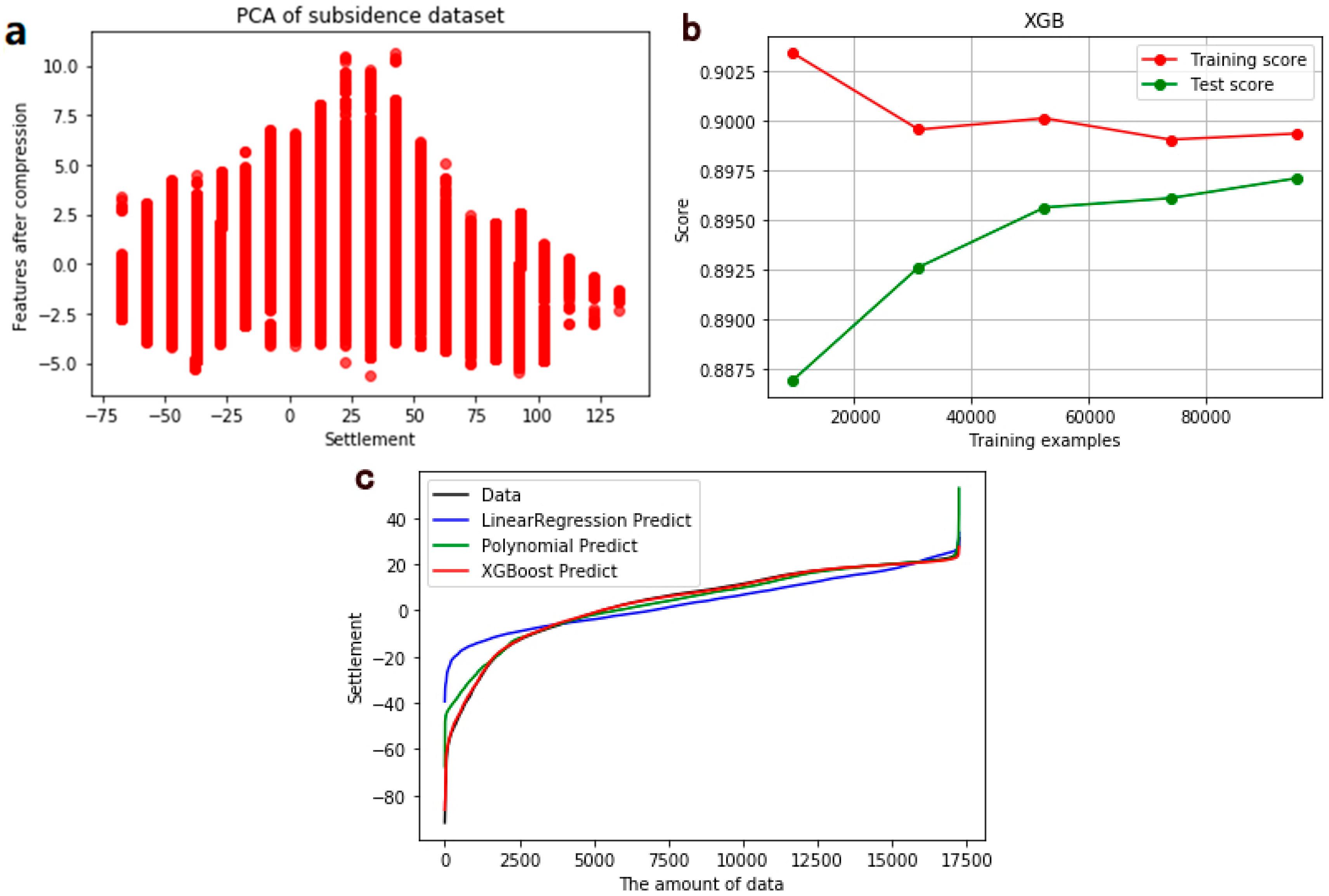
The data set composed of 119,086 PS points is input into XGBoost. Using the learning curve to observe the potential of XGBoost on the data set, the results are shown in Figure 7b. The performance on the training set shows the learning ability of the model, and the performance on the test set shows the generalization ability of the model. The performance of the model on the test set generally does not exceed the training set. We need to adjust the parameters to make the learning curve of the test set close to the learning curve of the training set. As can be seen from Figure 7b, with the increase of data amount, the learning curve of test set drops rapidly and then remains stable. Therefore, in order to get a better prediction effect in this experiment, the learning curve of the training set needs to be adjusted upward, and the learning curve of the test set should be close to the learning curve of the training set to obtain the best effect.
In order to predict the subsidence amount of the study area in 2018, we divided the data set into two new data sets. The land subsidence amount, groundwater level change, IBI, and thickness of the Quaternary deposit of 57,462 PS points from 2016 to 2017 were constructed into the first data set. In addition, the first data set was divided into a 70% train set and 30% test set. The land subsidence amount, groundwater level change, IBI, and thickness of the Quaternary deposit of 61,624 PS points in 2018 were constructed into the second data set. The second data set contains more data than the first data set. More PS points are selected to test the prediction ability of the model for the subsidence amount of unknown locations. In this way, we explore the universality of the model and prove the rationality of the prediction. First, we input the first data set into XGBoost to adjust the parameters of the model. When the accuracy of model reached the maximum, the prediction model was established. Then, we input the second data set into the model trained with the first data set to predict the land subsidence amount in 2018.
The XGBoost algorithm sets many parameters when compiling, but not all parameters need to be adjusted. Eight parameters have a greater impact on the model effect. The more the number of the weak evaluator, the stronger the learning ability of the model. The model obtains high accuracy, but it is easy to overfit. Therefore, num_round should be controlled within a reasonable range, generally not more than 600. The eta is called the learning rate, which is used to control the rate of iterations and prevent overfitting. The eta and num_round influence each other, and both need to be searched by GridSearchCV to get the optimal solution. In reality, data amount is huge, and the calculation of the tree model is very slow. Therefore, random sampling need to be performed. The subsample is used to control the proportion of the extraction of example. Among other parameters, xgb_model is an important parameter for selecting a weak evaluator. The objective is used to select the loss function. The alpha and lambda control the parameters of L1 regularization term and L2 regularization term respectively. The gamma is used to stop the tree from growing. The adjustment results of the parameters are shown in Table 3.

4. Results and Discussion

4.1. InSAR Results and Verification

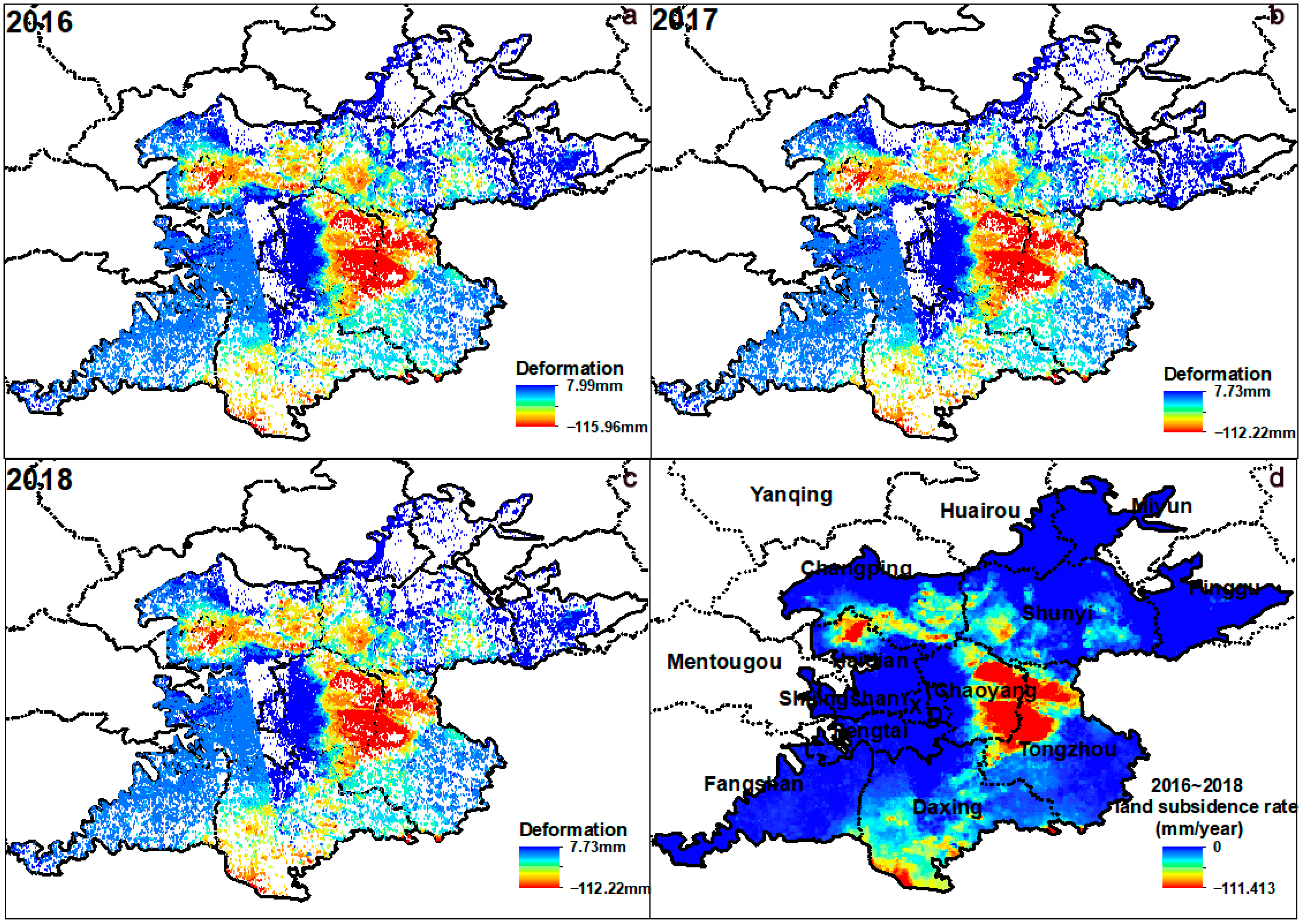
The average vertical deformation rate in the Beijing Plain from 2016 to 2018 is shown in Figure 2d. From 2016 to 2018, the maximum land subsidence rate in the Beijing Plain was 111.413 mm/y. The area with a land subsidence rate greater than 30 mm/y reached 770.1 km2, which accounted for 12.05% in the Beijing Plain. There was uneven land subsidence in the Beijing Plain. The eastern Chaoyang, northwestern Tongzhou, northwestern Haidian, southeastern Changping, western Shunyi, and southern Daxing had serious land subsidence. Among them, eastern Chaoyang and northwestern Tongzhou were heavy disaster areas. There were subsidence funnels in the study area.
From 2016 to 2017, the variation range of deformation in the Beijing Plain decreased slightly, and the maximum subsidence amount dropped from 115.96mm to 112.22 mm (Figure 2). The maximum subsidence amount from 2017 to 2018 remained almost stable, and variation range of deformation remained consistent. The area with the maximum average annual subsidence in the Beijing Plain was located in eastern Chaoyang and northwestern Tongzhou. The maximum average annual subsidence amount was more than 110 mm.
The monitoring values of 35 leveling benchmarks in the Beijing Plain from 2016 to 2018 were selected to verify the vertical deformation obtained by Sentinel-1 data. Taking each benchmark as the center, the PS points in the buffer with a radius of 150 m were extracted. We compared the value of leveling benchmarks with vertical deformation of PS points, and the result is shown in Figure 3. The correlation coefficient between the InSAR monitoring values and the leveling values is 0.9046, and the absolute error is between 1.52 mm/y and 28.72 mm/y. From the verification results, InSAR monitoring values are in good agreement with leveling values.

4.2. The Relationship between Influencing Factors and Land Subsidence

4.2.1. The Influence of Urban Construction on Land Subsidence

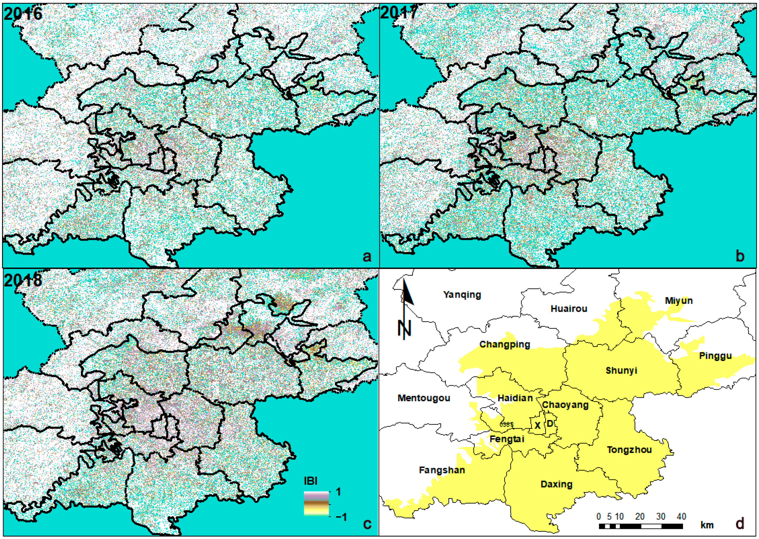
The IBI in the Beijing Plain is shown in Figure 4. It can be seen from Figure 4 that the IBI changes year by year. The color in the figure gets darker and the number of index close to 1 increases. In areas with severe land subsidence, IBI is also close to 1. However, it does not mean that the larger the IBI, the more serious the land subsidence. The IBI index is positive in many areas with severe subsidence. The rapid development of urban construction in Beijing has a certain impact on land subsidence.

4.2.2. The Influence of Thickness of the Quaternary Deposit on Land Subsidence

Soil is the material basis for land subsidence. When a large amount of groundwater is mined and the groundwater level changes to a certain extent, the pore water pressure of the clay layer will decrease and the effective stress will increase. Then the soil layer will compress and cause land subsidence. The deformation of the soil layer depends on the thickness, type, age, and structure of the soil. Figure 5 shows the distribution of thickness of the Quaternary deposit in the Beijing Plain and the contour lines of the cumulative settlement from 2016 to 2018. Thickness of the Quaternary deposit of 150–200 m and 100–150 m covers the larger range, followed by thickness of the Quaternary deposit of 50–100 m, and thickness of the Quaternary deposit of 200–250 m covers the smallest range. We found that land subsidence mainly occurs at a thickness of the Quaternary deposit of 150–200 m.

4.2.3. The Influence of Different Aquifers on Land Subsidence

Random Forest and XGBoost have a better exploration effect on the data set. R2 is used as the evaluation index of accuracy. The R2 formula is as follows:
R2 = 1 − SSresidual/SStotal
SSresidual is the residual sum of squares, and it is the sum of the squares of the difference between the predicted value and the label; SStotal is the total sum of squares, and it is the sum of the squares of the difference between the mean of the label and the label.
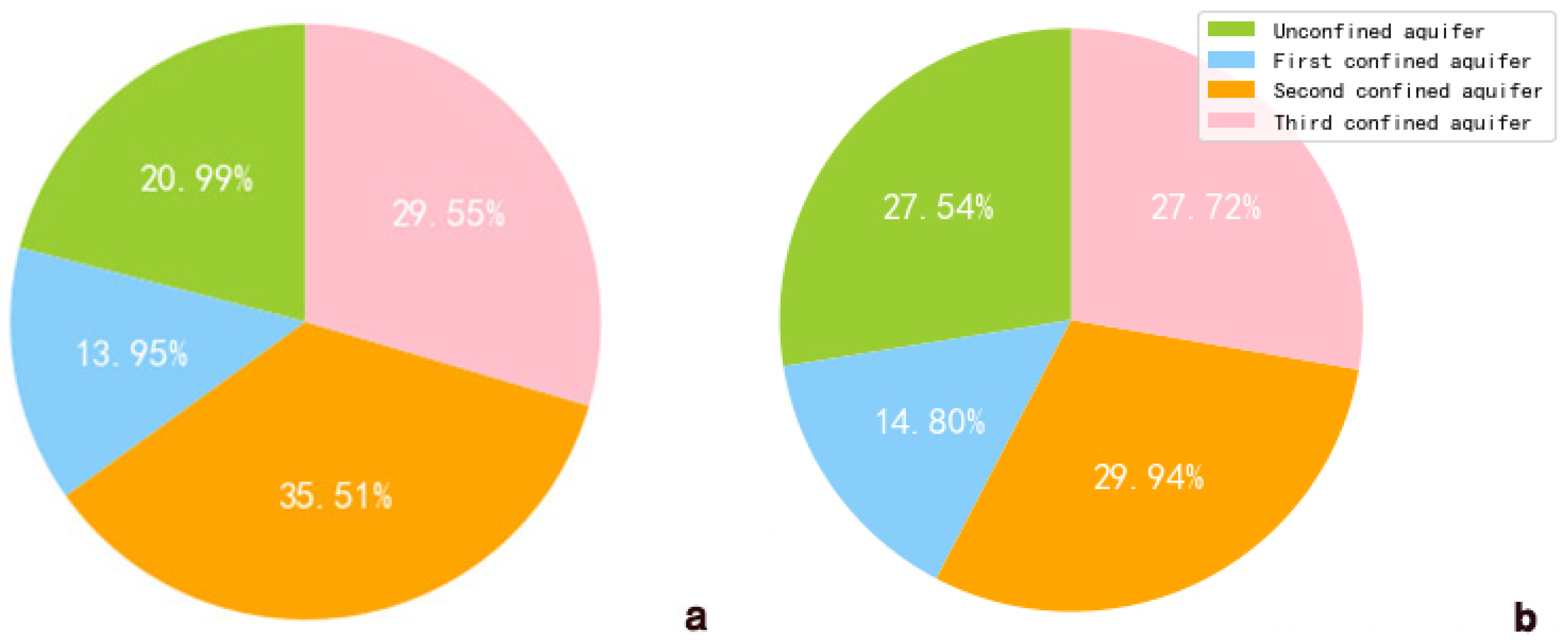
The accuracy of Random Forest reached 0.9739, and the accuracy of XGBoost reached 0.9657. The effect weight of each feature is shown in Figure 6. The same data had different effect weight in different models, but the general trend of the proportion was the same. The second confined aquifer had the greatest impact on land subsidence, with a contribution rate of 29.94% in Random Forest and 35.51% in XGBoost. The least impact was the unconfined aquifer.

4.2.4. The Nonlinear Relationship between Influencing Factors and Land Subsidence

In LinearRegression, the performance of the data set was very poor, and accuracy was only 0.4234. Only few features were predicted correctly, so there was a nonlinear relationship between the feature and label. The data distribution after PCA processing is shown in Figure 7a. It can be seen that there was no obvious linear relationship between the label and the feature, which further proved that the data was nonlinear.
PolynomialFeatures was used to help LinearRegression solve nonlinear data. In the case of the data set without any preprocessing, PolynomialFeatures was performed. When parameter degree was 5, the accuracy reached the maximum of 0.7667. At the same time, a complex polynomial consisting of hundreds of coefficients was generated. We used StandardScaler of preprocessing to normalize the data and input data into PolynomialFeatures. The parameter degree still achieved the maximum accuracy at 5, and the accuracy was 0.7757. The improvement was minimal. The prediction effect of subsidence amount has not reached the ideal accuracy, so we need a nonlinear model to predict subsidence amount.

4.3. The Result of Subsidence Prediction Model

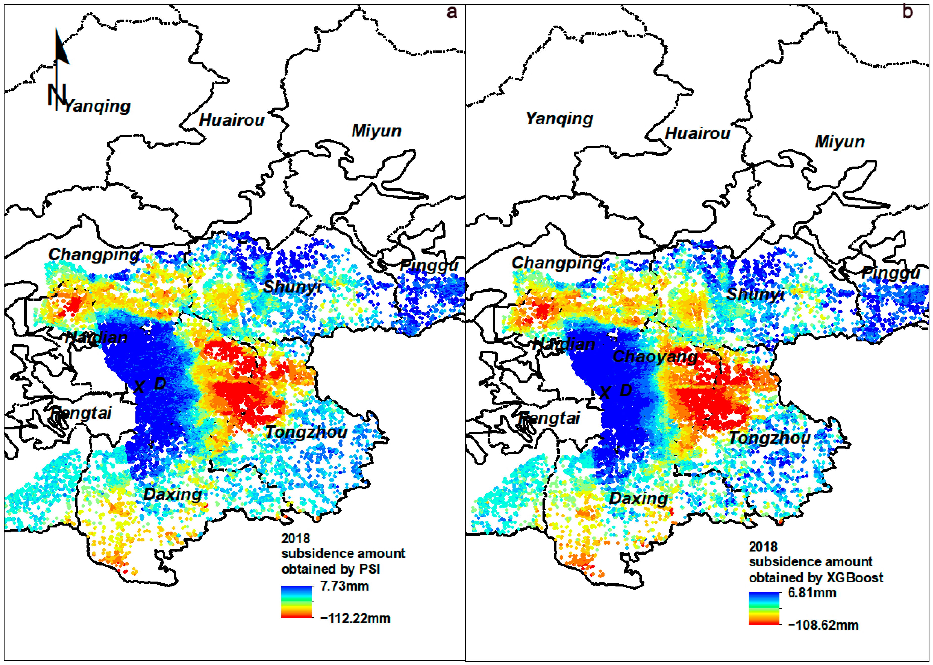
The first data set was input into XGBoost. After adjusting the parameters of XGBoost model many times, a model with high accuracy in predicting settlement was obtained. The prediction accuracy of subsidence amount reached 0.9700 on the training set and 0.9514 on the test set. There was no over-fitting phenomenon. Only few points in the study area had deviations in the prediction of subsidence amount. It can be seen from Figure 7c that the model predicts the subsidence amount of extreme points poorly, and the prediction effect of the remaining points is better. For the same data set, the test set performs best in XGBoost, and the prediction results of other algorithms are poor. The second data set for predicting subsidence amount performed well in the model trained on the first data set. The R2 was 0.9431, and the mean square error was controlled at 15.97. The mean square error can evaluate the degree of data change. The smaller the MSE value is, the better the accuracy of the prediction model is to describe the experimental data. The prediction result is shown in Figure 8b.

5. Conclusions

The land subsidence was affected by many factors. We selected the major influencing factors to research the relationship with land subsidence and predict the subsidence amount in the Beijing Plain through influencing factors. The conclusions are as follows.
(1)
The PSI results agreed well with the leveling benchmark results. The correlation coefficient was 0.9046, and the minimum absolute error and maximum absolute error were 1.52 mm/y and 28.72 mm/y, respectively. From 2016 to 2018, the maximum subsidence rate in the Beijing Plain had reached 115.96 mm/y. The land subsidence was serious in eastern Chaoyang and northwestern Tongzhou.
(2)
We found that the area where thickness of the Quaternary deposit reached 150–200 m was prone to land subsidence. Among the four aquifers, the groundwater exploitation of the second confined aquifer had the greatest impact on land subsidence in the Beijing Plain, with a contribution rate of 29.94% in random forest and 35.51% in XGBoost. Through Linear Regression and PCA, the relationship between groundwater level change, thickness of the Quaternary deposit, IBI, and land subsidence was nonlinear.
(3)
Compared with the subsidence amount obtained by PS-InSAR, the prediction accuracy of subsidence amount based on XGBoost method reached 0.9431, and the mean square error was controlled at 15.97. The accuracy of the training set and the test set on the model were similar, and there was no overfitting phenomenon. The prediction effect of XGBoost was good and reasonable. Only few points had deviations in the prediction of subsidence amount. Our research extends the application range of the land subsidence prediction model without complex hydrogeological parameters. It provides a new idea for land subsidence prediction.
The model constructed in this experiment also has potential shortcomings. Factors such as groundwater hysteresis, faults, lithology, and other influencing factors have not been taken into consideration, and it is not clear whether the input of other influencing factors will obtain a better prediction effect. These issues will be considered in future research.

Author Contributions

L.S. designed the experiments, performed the algorithm, and wrote the original paper. B.C. made important suggestions on writing the paper, and provided data. H.G. provided guidance. C.Z. provided guidance and data. All authors have read and agreed to the published version of the manuscript.

Funding

This work was founded by National Natural Science Foundation of China (No. 41930109/D010702, 41771455/D010702), Beijing Outstanding Young Scientist Program (No. BJJWZYJH01201910028032), Beijing Youth Top Talent Project, Beijing Municipal Natural Science Foundation (No. 8182013), National “Double-Class” Construction of University Projects, the program of Beijing Scholars and Beijing Postdoctoral Research Foundation (No. 2018M641407).

Acknowledgments

We are grateful for the ground subsidence level measurement data provided by the Beijing Institute of Hydrogeology and Engineering Geology.

Conflicts of Interest

The authors declare no conflict of interest.

References

  1. Galloway, D.L.; Erkens, G.; Kuniansky, E.L.; Rowland, J.C. Preface: Land subsidence processes. Hydrogeol. J. 2016, 24, 547–550. [Google Scholar] [CrossRef] [Green Version]
  2. Strozzi, T.; Wegmuller, U. Land subsidence in Mexico City mapped by ERS differential SAR interferometry. IEEE Int. Geosci. Remote Sens. Symp. 1999, 4, 1940–1942. [Google Scholar]
  3. Yamamoto, S. Land Subsidence and its Problems: With reference to the results of International Symposium on Land Subsidence, Tokyo, 1969. J. Geogr. 1970, 78, 471–482. [Google Scholar] [CrossRef]
  4. Hu, R.L.; Yue, Z.Q.; Wang, L.C.; Wang, S.J. Review on current status and challenging issues of land subsidence in China. Eng. Geol. 2004, 76, 65–77. [Google Scholar] [CrossRef]
  5. Rosi, A.; Tofani, V.; Agostini, A.; Tanteri, L.; Tacconi Stefanelli, C.; Catani, F.; Casagli, N. Subsidence mapping at regional scale using persistent scatters interferometry (PSI): The case of Tuscany region (Italy). Int. J. Appl. Earth Obs. Geoinf. 2016, 52, 328–337. [Google Scholar] [CrossRef]
  6. Nutalaya, P.; Yong, R.N.; Chumnankit, T.; Buapeng, S. Land Subsidence in Bangkok during 1978–1988. Sea-Level Rise Coast. Subsid. 1996, 2, 105–130. [Google Scholar]
  7. Hawkes, A.D.; Horton, B.P.; Nelson, A.R.; Vane, C.H.; Sawai, Y. Coastal subsidence in Oregon, USA, during the giant Cascadia earthquake of AD 1700. Quat. Sci. Rev. 2011, 30, 364–376. [Google Scholar] [CrossRef] [Green Version]
  8. Mingliang, G.; Huili, G.; Beibei, C.; Xiaojuan, L.; Chaofan, Z.; Min, S.; Yuan, S.; Zheng, C.; Guangyao, D. Regional Land Subsidence Analysis in Eastern Beijing Plain by InSAR Time Series and Wavelet Transforms. Remote Sens. 2018, 10, 365. [Google Scholar]
  9. Zuo, J.; Gong, H.; Chen, B.; Liu, K.; Zhou, C.; Ke, Y. Time-series evolution patterns of land subsidence in the Eastern Beijing Plain, China. Remote Sens. 2019, 11, 539. [Google Scholar] [CrossRef] [Green Version]
  10. Yan, Y.; Yuan, J. Analysis and Outlook of the Land Subsidence in Beijing. Urban Geol. 2012, 7, 2. [Google Scholar]
  11. Zhou, C.; Gong, H.; Chen, B.; Gao, M.; Shi, M. Land Subsidence Response to Different Land Use Types and Water Resource Utilization in Beijing-Tianjin-Hebei, China. Remote Sens. 2020, 12, 457. [Google Scholar] [CrossRef] [Green Version]
  12. Xu, Y.S.; Ma, L.; Du, Y.J.; Shen, S.L. Analysis of urbanisation-induced land subsidence in Shanghai. Nat. Hazards 2012, 63, 1255–1267. [Google Scholar] [CrossRef]
  13. Chai, J.C.; Shen, S.L.; Zhu, H.H.; Zhang, X.L. Land subsidence due to groundwater drawdown in Shanghai. Geotechnique 2004, 56, 143–147. [Google Scholar] [CrossRef]
  14. Yan, X.X.; Gong, S.L.; Zeng, Z. Relationship between building density and land subsidence in Shanghai urban zone. Hydrogeol. Eng. Geol. 2002. [Google Scholar] [CrossRef]
  15. Yang, Q.; Ke, Y.; Zhang, D.; Chen, B.; Gong, H.; Lv, M.; Zhu, L.; Li, X. Multi-Scale Analysis of the Relationship between Land Subsidence and Buildings: A Case Study in an Eastern Beijing Urban Area Using the PS-InSAR Technique. Remote Sens. 2018, 10, 1006. [Google Scholar] [CrossRef] [Green Version]
  16. Bamler, R.; Hartl, P. Synthetic aperture radar interferometry. Inverse Probl. 1999, 14, 4. [Google Scholar] [CrossRef]
  17. Rosen, P.A.; Hensley, S.; Joughin, I.R.; Li, F.K.; Madsen, S.N.; Rodriguez, E.; Goldstein, R.M. Synthetic aperture radar interferometry. Proc. IEEE 2002, 88, 333–382. [Google Scholar] [CrossRef]
  18. Hanssen, R.F. Radar Interferometry Data Interpretation and Error Analysis; Springer Science and Business Media: Dordrecht, The Netherlands, 2001. [Google Scholar]
  19. Amelung, F.; Galloway, D.L.; Bell, J.W.; Zebker, H.A.; Laczniak, R.J. Sensing the ups and downs of Las Vegas: InSAR reveals structural control of land subsidence and aquifer-system deformation. Geology 1999, 27, 483–486. [Google Scholar] [CrossRef]
  20. Chaussard, E.; Wdowinski, S.; Cabral-Cano, E.; Amelung, F. Land subsidence in central Mexico detected by ALOS InSAR time-series. Remote Sens. Environ. 2014, 140, 94–106. [Google Scholar] [CrossRef]
  21. Bawden, G.W.; Thatcher, W.; Stein, R.S.; Hudnut, K.W.; Peltzer, G. Tectonic contraction across Los Angeles after removal of groundwater pumping effects. Nature 2001, 412, 812–815. [Google Scholar] [CrossRef]
  22. Ferretti, A.; Prati, C.; Rocca, F. Permanent scatterers in SAR interferometry. IEEE Trans. Geosci. Remote Sens. 2001, 39, 8–20. [Google Scholar] [CrossRef]
  23. Bürgmann, R.; Hilley, G.; Ferretti, A.; Novali, F. Resolving vertical tectonics in the San Francisco Bay Area from permanent scatterer InSAR and GPS analysis. Geology 2006, 34, 221–224. [Google Scholar] [CrossRef] [Green Version]
  24. Ge, L.; Ng, H.M.; Li, X.; Abidin, H.Z. Land subsidence characteristics of Bandung Basin as revealed by ENVISAT ASAR and ALOS PALSAR interferometry. Remote Sens. Environ. 2014, 154, 46–60. [Google Scholar] [CrossRef]
  25. Hooper, A.; Segall, P.; Zebker, H. Persistent scatterer interferometric synthetic aperture radar for crustal deformation analysis, with application to Volcán Alcedo, Galápagos. J. Geophys. Res. 2007, 112, B07407. [Google Scholar] [CrossRef] [Green Version]
  26. Chen, B.; Gong, H.; Chen, Y.; Li, X.; Zhao, X. Land subsidence and its relation with groundwater aquifers in Beijing Plain of China. Sci. Total Environ. 2020, 735, 139111. [Google Scholar] [CrossRef]
  27. Gong, H.; Zhang, Y.; Li, X.; Lu, X.; Chen, B.; Gu, Z. Land subsidence research in Beijing based on the permanent Scatterers InSAR technology. China Acad. J. Electron. Publ. House 2009, 19, 1261–1266. [Google Scholar]
  28. Liu, G.X.; Zhang, R.; Li, T.; Yu, B.; Nie, Y.J. Extracting 3D ground deformation velocity field by multi-platform persistent scatterer SAR interferometry Chinese. J. Geophys. 2012, 55, 2598–2610. (In Chinese) [Google Scholar]
  29. Azqueta-Gavaldon, A. Developing news-based Economic Policy Uncertainty index with unsupervised machine learning. Econ. Lett. 2017, 158, 47–50. [Google Scholar] [CrossRef] [Green Version]
  30. Farmer, J.D.; Packard, N.H.; Perelson, A.S. The immune system, adaptation, and machine learning. Phys. D Nonlinear Phenom. 1986, 22, 187–204. [Google Scholar] [CrossRef]
  31. Zhao, K.; Chen, S. Study on Artificial Neural Network Method for Ground Subsidence Prediction of Metal Mine. Procedia Earth Planet. Sci. 2011, 2, 177–182. [Google Scholar] [CrossRef] [Green Version]
  32. Zamanirad, M.; Sarraf, A.; Sedghi, H.; Saremi, A.; Rezaee, P. Modeling the Influence of Groundwater Exploitation on Land Subsidence Susceptibility Using Machine Learning Algorithms. Nat. Resour. Res. 2019, 1–15. [Google Scholar] [CrossRef]
  33. Rahmati, O.; Golkarian, A.; Biggs, T.; Keesstra, S.; Mohammadi, F.; Daliakopoulos, I.N. Land subsidence hazard modeling: Machine learning to identify predictors and the role of human activities. J. Environ. Manag. 2019, 236, 466–480. [Google Scholar] [CrossRef] [PubMed]
  34. Rahmati, O.; Falah, F.; Naghibi, S.A.; Biggs, T.; Soltani, M.; Deo, R.C.; Cerdà, A.; Mohammadi, F.; Bui, D.T. Land subsidence modelling using tree-based machine learning algorithms. Sci. Total Environ. 2019, 672, 239–252. [Google Scholar] [CrossRef] [PubMed]
  35. Tsangaratos, P.; Ilia, I.; Loupasakis, C. Land Subsidence Modelling Using Data Mining Techniques. The Case Study of Western Thessaly, Greece. In Natural Hazards GIS-Based Spatial Modeling Using Data Mining Techniques; Springer: Berlin/Heidelberg, Germany, 2019. [Google Scholar]
  36. Zhou, C.; Gong, H.; Chen, B.; Li, X.; Li, J.; Wang, X.; Gao, M.; Si, Y.; Guo, L.; Shi, M. Quantifying the contribution of multiple factors to land subsidence in the Beijing Plain, China with machine learning technology. Geomorphology 2019, 335, 48–61. [Google Scholar] [CrossRef]
  37. Zhou, Z.H. Ensemble Methods: Foundations and Algorithms; Taylor & Francis, CRC Press: Boca Raton, FL, USA, 2012. [Google Scholar]
  38. Blaszczynski, J.; Stefanowski, J. Neighbourhood sampling in bagging for imbalanced data. Neurocomputing 2015, 150, 529–542. [Google Scholar] [CrossRef]
  39. Ziba, M.; Tomczak, S.K.; Tomczak, J.M. Ensemble boosted trees with synthetic features generation in application to bankruptcy prediction. Expert Syst. Appl. 2016, 58, 93–101. [Google Scholar] [CrossRef]
  40. Tang, B.; Chen, Q.; Wang, X.; Wang, X. Reranking for Stacking Ensemble Learning. Neural Inf. Process. Theory Algorithm 2010. [Google Scholar] [CrossRef]
  41. Breiman, L. Random Forests. Mach. Learn. 2001, 45, 5–32. [Google Scholar] [CrossRef] [Green Version]
  42. Son, J.; Jung, I.; Park, K.; Han, B. Tracking-by-Segmentation with Online Gradient Boosting Decision Tree. In Proceedings of the 2015 IEEE International Conference on Computer Vision, Santiago, Chile, 7–13 December 2015. [Google Scholar] [CrossRef]
  43. Chen, T.; Guestrin, C. XGBoost: A Scalable Tree Boosting System. In Proceedings of the KDD’16: 22nd ACM SIGKDD International Conference on Knowledge Discovery and Data Mining, San Francisco, CA, USA, 13–17 August 2016; Volume 8, pp. 785–794. [Google Scholar]
  44. Bi, Y.; Xiang, D.; Ge, Z.; Li, F.; Jia, C.; Song, J. An Interpretable Prediction Model for Identifying N 7-Methylguanosine Sites Based on XGBoost and SHAP. Mol. Ther. Nucleic Acids 2020. [Google Scholar] [CrossRef]
  45. Xu, M.; Wei, D.; Zhu, T.; Zhang, Y. Box-Office Revenue Predictions Based on XGBoost and Sentiment Analysis. World Sci. Res. J. 2020, 6, 11. [Google Scholar]
  46. Wang, S.; Liu, S.; Zhang, J.; Che, X.; Yuan, Y.; Wang, Z.; Kong, D. A New Method of Diesel Fuel Brands Identification: SMOTE Oversampling Combined with XGBoost Ensemble Learning. Fuel 2020, 282, 118848. [Google Scholar] [CrossRef]
  47. Yuanzhang, L.; Ruixin, W.; Xu, W.; Shufang, W.; Liya, W.; Yijiao, C. Preliminary Study on Selection Schemes of Groundwater Environmental Background Values in Beijing Area. Urban Geol. 2019, 14, 4. [Google Scholar]
  48. Yu, L. Division of Water-bearing Zones and Compressible Layers in Beijing’s Land Subsidence Areas. City Geol. 2007, 2, 1. [Google Scholar]
  49. Chen, B.; Gong, H.; Lei, K.; Li, J.; Zhou, C.; Gao, M. Land subsidence lagging quantification in the main exploration aquifer layers in Beijing plain, China. Int. J. Appl. Earth Obs. Geoinf. 2019, 75, 54–67. [Google Scholar] [CrossRef]
  50. Deren, L.I. Progress of Permanent Scatterer Interferometry. Geomat. Inf. Sci. Wuhan Univ. 2004, 29, 8. [Google Scholar]
  51. Hooper, A.; Zebker, H.; Segall, P.; Kampes, B. A new method for measuring deformation on Volcanoes and other natural terrains using InSAR Persistent Scatterers. Geophys. Res. Lett. 2004, 31, 1–5. [Google Scholar] [CrossRef]
  52. Xu, H. A new index for delineating built-up land features in satellite imagery. Int. J. Remote Sens. 2008, 29, 4269–4276. [Google Scholar] [CrossRef]
  53. Huete, A.R. A soil-adjusted vegetation index (SAVI). Remote Sens. Enviorn. 1988, 25, 295–309. [Google Scholar] [CrossRef]
  54. Xu, H. Modification of normalised difference water index (NDWI) to enhance open water features in remotely sensed imagery. Int. J. Remote Sens. 2006, 27, 3025–3033. [Google Scholar] [CrossRef]
  55. Zha, Y.; Gao, J.; Ni, S. Use of normalized difference built-up index in automatically mapping urban areas from TM imagery. Int. J. Remote Sens. 2003, 24, 583–594. [Google Scholar] [CrossRef]
  56. Ritov, Y. Estimation in a Linear Regression Model with Censored Data. Ann. Stat. 1990, 18, 303–328. [Google Scholar] [CrossRef]
  57. Jolliffe, I.T. Principal Component Analysis. J. Mark. Res. 2002, 87, 513. [Google Scholar]
  58. Oliphant, T.E. Python for Scientific Computing. Comput. Sci. Eng. 2007, 9, 10–20. [Google Scholar] [CrossRef] [Green Version]
  59. Aiken, L.S.; West, S.G.; Pitts, S.C. Multiple Linear Regression. In Handbook of Psychology; John Wiley & Sons, Inc.: Hoboken, NJ, USA, 2003. [Google Scholar]
  60. Chen, B. Polynomial Regression. Springer Texts Stats 1986, 235–268. [Google Scholar]
  61. Breiman, L. Bagging predictors. Mach. Learn. 1996. [Google Scholar] [CrossRef] [Green Version]
  62. Lerman, P.M. Fitting Segmented Regression Models by Grid Search. Appl. Stats. 1980, 29, 77–84. [Google Scholar] [CrossRef]
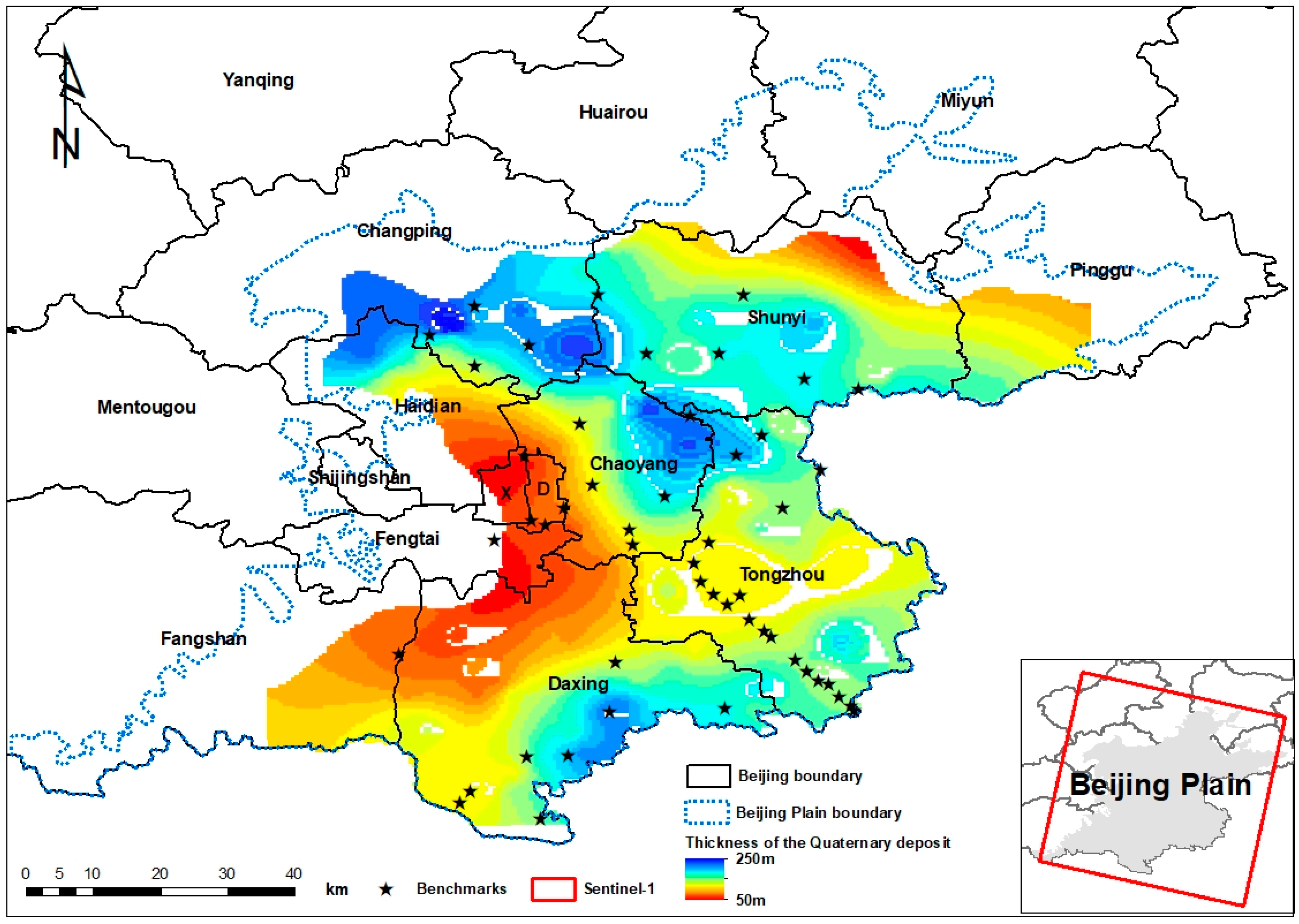
Figure 1. Location of the study area (the map of top left shows the location of Beijing and the distribution of thickness of the Quaternary deposit).
Remotesensing 12 04044 g001
Figure 2. Deformation in the Beijing Plain from 2016 to 2018. (ac) show the annual deformation between 2016 and 2018 in Beijing Plain; (d) is the average vertical subsidence rate in the Beijing Plain from 2016 to 2018, and the subsidence rate is the average of the annual settlement for 3 years.
Remotesensing 12 04044 g002
Figure 3. Comparison of InSAR-measured and leveling-measured velocity. (a) is the mean velocities from 2016 to 2018; (b) show the comparison results from 2016 to 2018.
Remotesensing 12 04044 g003
Figure 4. IBI in the Beijing Plain from 2016 to 2018. (ac) show the IBI inversion results of the Beijing Plain area from 2016 to 2018; (d) shows the regional distribution in the Beijing Plain.
Remotesensing 12 04044 g004
Figure 5. Overlay of the thickness of the Quaternary deposit in the Beijing Plain and the cumulative subsidence from 2016 to 2018.
Remotesensing 12 04044 g005
Figure 6. Weight distribution of different aquifers influencing land subsidence. (a) Based on the Random Forest model; (b) Based on the XGBoost model.
Remotesensing 12 04044 g006
Figure 7. Machine learning results. (a) The result of the first dataset for PCA processing; (b) The learning potential of 119,086 PS points in XGBoost; (c) Settlement predictions for the dataset on different models from 2016 to 2017.
Remotesensing 12 04044 g007
Figure 8. Vertical subsidence amount of 61,624 PS points in 2018. (a) The result of PSI; (b) The result of XGBoost.
Remotesensing 12 04044 g008
Table 1. The LinearRegression parameters.
Fifit_InterceptNormalizeCopy_Xn_Jobs
TrueFalseTrueNone
Table 2. The PolynomialFeatures parameters.
DegreeInteraction_OnlyInclude_Bias
5FalseTrue
Table 3. The XGBoost parameters.
Num_RoundEtaSubsamplexgb_ModelObjectiveAlphaLambdaGamma
6000.71gbtreereg:linear016
Publisher’s Note: MDPI stays neutral with regard to jurisdictional claims in published maps and institutional affiliations.