Using Deep Learning for Visual Navigation of Drone with Respect to 3D Ground Objects

Abstract

In the paper, visual navigation of a drone is considered. The drone navigation problem consists of two parts. The first part is finding the real position and orientation of the drone. The second part is finding the difference between desirable and real position and orientation of the drone and creation of the correspondent control signal for decreasing the difference. For the first part of the drone navigation problem, the paper presents a method for determining the coordinates of the drone camera with respect to known three-dimensional (3D) ground objects using deep learning. The algorithm has two stages. It causes the algorithm to be easy for interpretation by artificial neural network (ANN) and consequently increases its accuracy. At the first stage, we use the first ANN to find coordinates of the object origin projection. At the second stage, we use the second ANN to find the drone camera position and orientation. The algorithm has high accuracy (these errors were found for the validation set of images as differences between positions and orientations, obtained from a pretrained artificial neural network, and known positions and orientations), it is not sensitive to interference associated with changes in lighting, the appearance of external moving objects and the other phenomena where other methods of visual navigation are not effective. For the second part of the drone navigation problem, the paper presents a method for stabilization of drone flight controlled by autopilot with time delay. Indeed, image processing for navigation demands a lot of time and results in a time delay. However, the proposed method allows to get stable control in the presence of this time delay.

1. Introduction

The drone navigation problem [1,2,3,4,5,6,7,8,9,10,11] appeared during the development of systems for autonomous navigation of drones. The question arose about the possibility of determining the coordinates of the drone based on the image of the runway or the airfield control tower, or any characteristic building along the route of the drone.

However, the task of determining the coordinates of the camera with respect to three-dimensional (3D) object images can also be used for other conditions: indoor navigation or inside city navigation. Such navigation programs can be used both in tourist guide devices and in control of autonomous robots.

Usually, GPS (Global Positioning System) [1] and inertial navigation systems [2] are used to solve navigation problems. However, each of these navigation methods has its own drawbacks. Inertial systems tend to accumulate errors in the coordinates and angles of a drone during its flight. GPS also has a number of disadvantages, in particular, it has nonautonomous methods depending on correct operation of external satellites, it gives an accuracy of the order of several meters, and sometimes tens of meters, which is unacceptable for accurate navigation, such as, for example, taking off and landing a drone; also, GPS is unstable with respect to external noise or hacking.

Let us discuss the use of computer vision and deep learning for drone navigation. Despite the massive fascination with neural networks and their active implementation in computer applications, their use to determine the coordinates of objects or a camera relative to an object is studied much less often.

Most visual navigation techniques use landmarks to map and locate the camera. We usually use various functions to highlight correspondent features (key points) on video (for example, methods such as SIFT (scale-invariant feature transform) [3] or the Lucas-Kanade method [4]). From known points’ motion, we can find egomotion and three-dimensional (3D) environment reconstruction. Unfortunately, such features are not universal, for example, there is a problem of recognizing such point-like features, and to identify correspondent features during large camera egomotion, intrinsic features can be non-point-like, and so on.

We use deep learning and convolutional neural networks to identify such complex features and their correspondence. We can significantly reduce data processing time and improve accuracy, which is especially important for maneuvering a drone [5,6,7,8,9,10].

“PoseNet” [5] is based on the GoogLeNet architecture. It processes RGB (Red, Green, Blue, i.e., colour images) images and is modified so that all three softmax and fully connected layers are removed from the original model and replaced by regressors in the training phase. In the testing phase, the other two regressors of the lower layers are removed and the prediction is done solely based on the regressor on the top of the whole network.

For Bayesian PoseNet, Kendall et al. [6] propose a Bayesian convolutional neural network to estimate uncertainty in the global camera pose, which leads to improving localization accuracy. The Bayesian convolutional neural network is based on PoseNet architecture by adding dropout after the fully connected layers in the pose regressor and after one of the inception layers (layer 9) of the GoogLeNet architecture.

Long short-term memory (LSTM)-Pose [7] is otherwise similar to PoseNet but applies LSTM (a type of Recurrent Neural Network (RNN)) networks for output features coming from the final fully connected layer. In detail, it is based on utilizing the pre-trained GoogLeNet architecture as a feature extractor followed by four LSTM units applied in the up, down, left, and right directions. The outputs of LSTM units are then concatenated and fed to a regression module consisting of two fully connected layers to predict camera pose.

VidLoc [8] is a CNN (Convolution Neural Network)-based system based on short video clips. As in PoseNet and LSTM-Pose, VidLoc incorporates a similarly modified pre-trained GoogLeNet model for feature extraction. The output of this module is passed to bidirectional LSTM units predicting the poses for each frame in the sequence by exploiting contextual information in past and future frames [9].

In Reference [9], an encoder-decoder convolutional neural network (CNN) architecture was proposed for estimating camera pose (orientation and location) from a single RGB image. The architecture has an hourglass shape consisting of a chain of convolution and up-convolution layers followed by a regression part.

In Reference [10], similar to PoseNet, MapNet also learns a DNN (deep learning neural network) that estimates the 6-DoF (6 Degrees of Freedom) camera pose from an input RGB image on the training set via supervised learning. The main difference, however, is that MapNet minimizes both the loss of the per-image absolute pose and the loss of the relative pose between image pairs.

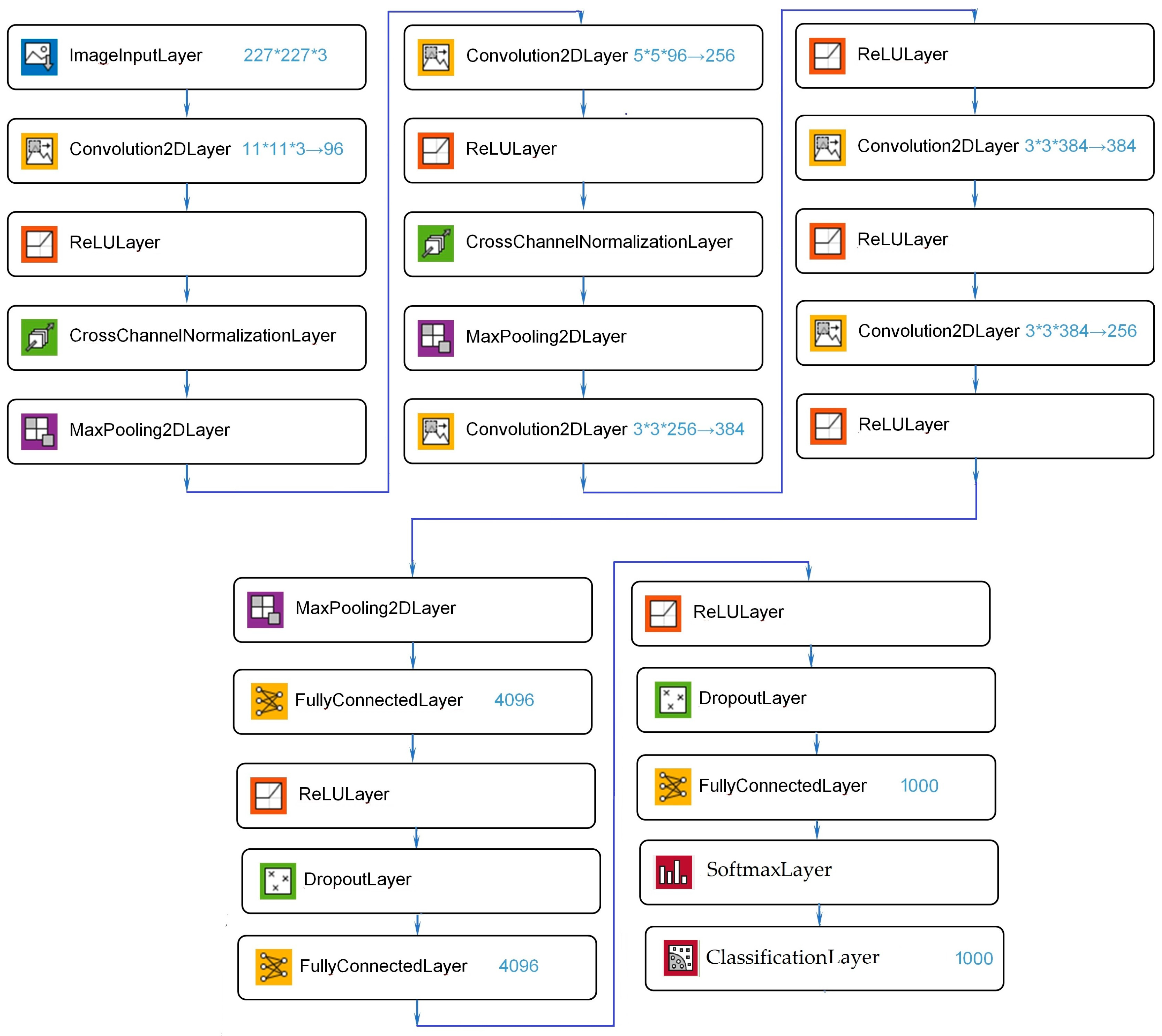
In this study, we used modified AlexNet (see Figure 1). AlexNet [12,13,14,15] is the name of a convolutional neural network (CNN), designed by Alex Krizhevsky and published with Ilya Sutskever and Krizhevsky’s doctoral advisor Geoffrey Hinton [12]. AlexNet competed in the ImageNet Large-Scale Visual Recognition Challenge on 30 September 2012, significantly outperforming other networks. In the original AlexNet, there are only 8 levels (5 convolutional and 3 fully connected). It is possible to load a pretrained version of the network trained on more than a million images from the ImageNet database [12,13,14,15]. The pretrained network can classify images into 1000 object categories, such as keyboard, mouse, pencil, and many animals. As a result, the network has learned rich feature representations for a wide range of images. The network has an image input size of 227 × 227.

2. Materials and Methods

There is a series of interesting papers [5,6] where the authors used deep learning and convolutional neural network to determine camera position and orientation. These papers are pioneer work in the application of deep learning techniques to navigation.

Unfortunately, this technology is used only for ground cameras, that can be placed on ground robots, ground vehicles, or pedestrians. More specifically, in their work [5,6], the authors determined the coordinates and angle of the camera using images of the Cambridge Landmarks building, filmed with a smartphone camera by pedestrians.

The flying camera was used in the current paper, unlike in References [5,6], where the authors used only the ground camera. So, in the current paper, we are able to analyze the applicability of deep learning technology for many more ranges of angles and coordinates.

In References [5,6,7,8,9], Cartesian coordinates and quaternions (logarithm of unit quaternions in Reference [10]) were used for description of the camera position and orientation. We used a description of the camera position and orientation that is more natural for images. It allows us to get better precision for the camera position and orientation. Indeed, such description provides the data which is easier and more natural for understanding by the artificial neural network.

In more detail, we considered the problem in which the camera can be located at a great distance (up to 1000 m) from the ground object landmark. Therefore, our method involves two stages: determining the position of the object on the image, and then determining the position and orientation of the camera using only a narrow neighborhood of the object.

This position and orientation of the camera is described (i) by two angles describing the camera optical axis rotation with respect to the ray (connecting the object with the camera optical center), (ii) by the distance between the camera optical center and the object, and (iii) by quaternions, describing two angles of the ray and one angle of the camera rotation around the ray.

For the two stages, as described above, we used the two artificial neural networks, which are built on the basis of AlexNet [12,13,14,15] with small changes in structure and training method.

3. Results

3.1. Deep Learning for Localization: Training and Validation of Dataset Formation

We considered the problem of determining three coordinates and three angles of rotation of the camera using the artificial neural network.

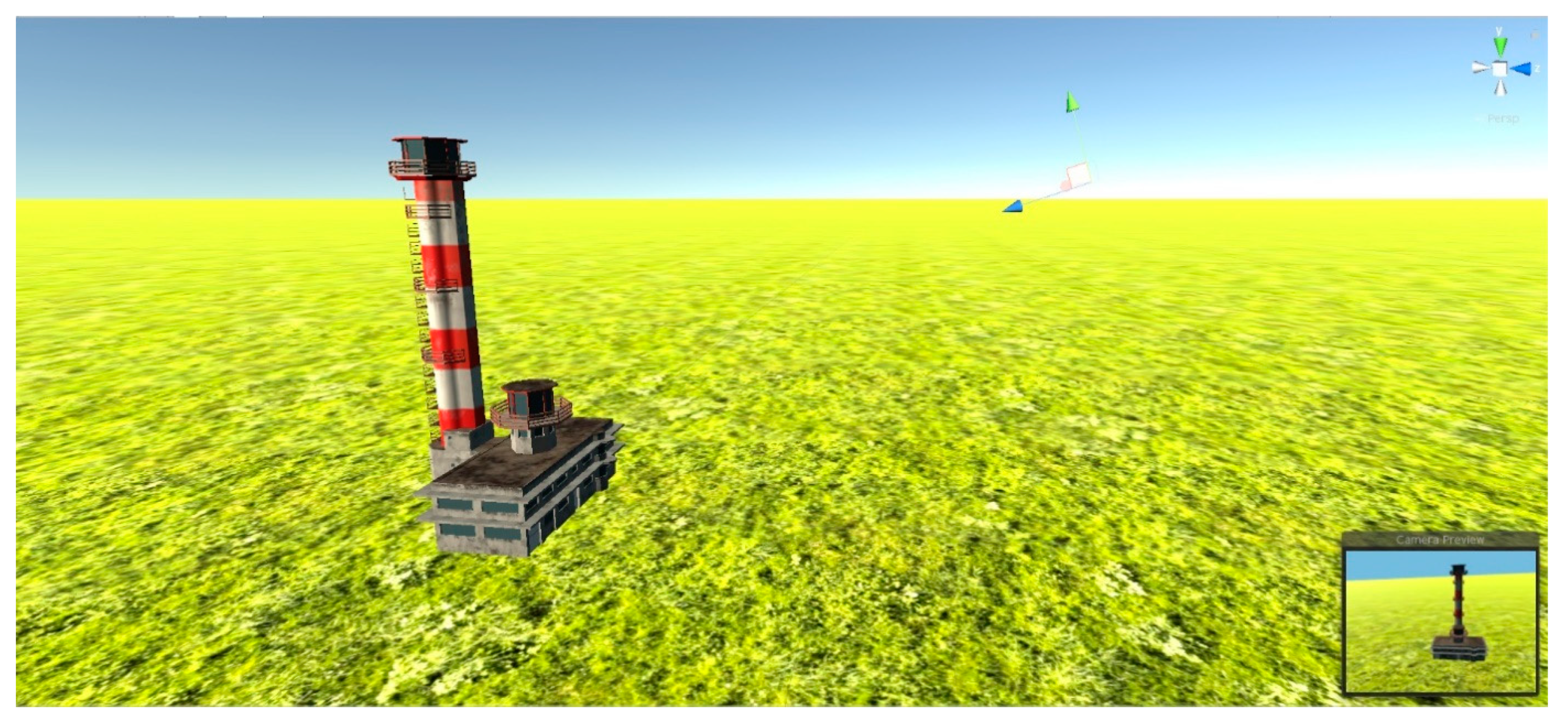
In the game application Unity, the model scene was created, containing an airport control tower in the middle of an endless green field (Figure 2).

In real life, any object is surrounded by dozens of others—houses, trees, roads, etc.—which give us additional information for orientation. We decided to make the task minimally dependent on additional landmarks, so that the neural network would only use the control tower building for navigation. Obviously, such a solution of a minimalistic task can be easily transformed to an environment where the landmark is surrounded by many other objects.

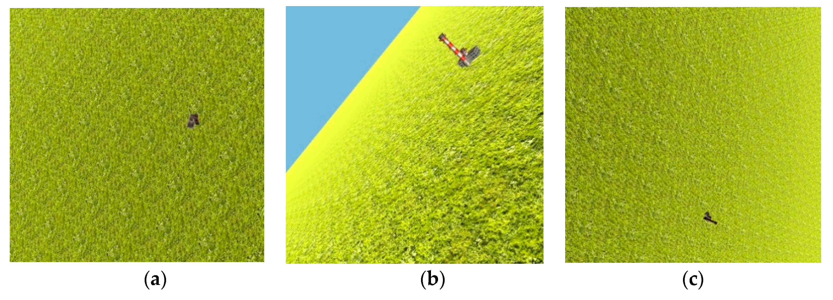
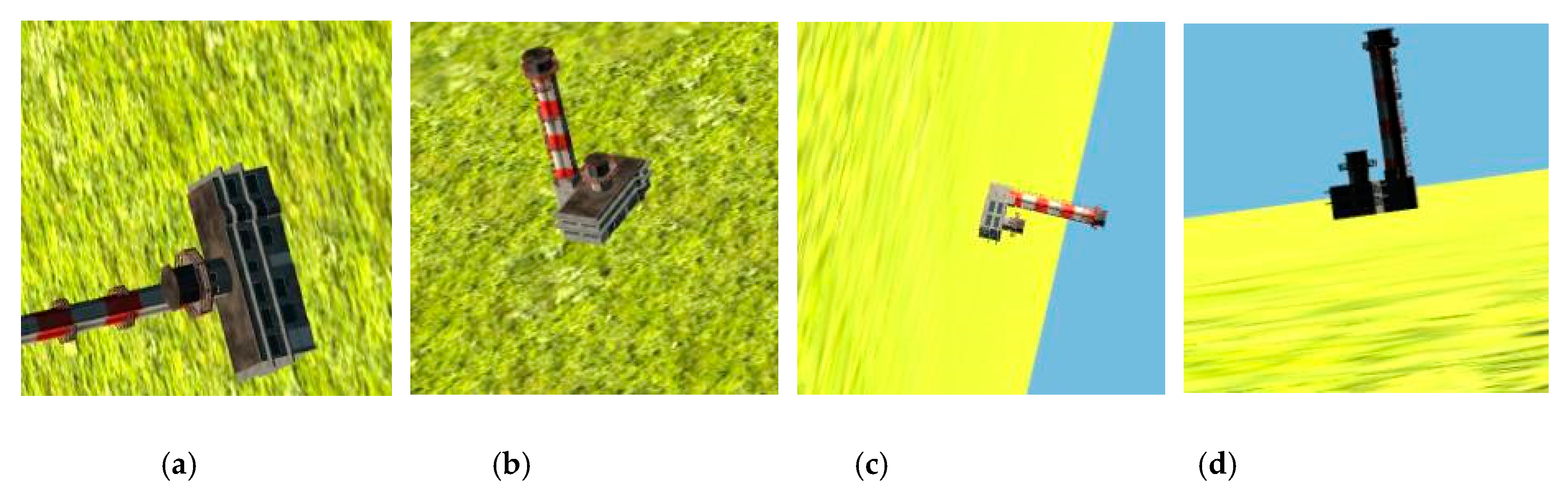
The basis of the landmark building (named as the object in further parts of the paper) was located at the origin of the ground coordinate system, and the virtual camera was randomly located above ground level at a distance from 200 to 1000 m from the object origin. The camera was always oriented so that the landmark building was completely included in the frame. In total, 6000 images were produced in pixel size of 2000 × 2000: 5000 for training and 1000 for validation (Figure 3).

All information about the coordinates of the camera in space and the location of the reference object on the image was automatically formed into a table, which was then used for training and validation of the neural network.

3.2. Two Stages and Two Artificial Neural Networks (ANN) for Finding the Drone Camera Position and Orientation

Since the obtained images have pixel size 2000 × 2000, which is too large for processing by a convolutional neural network, we split the task into two stages.

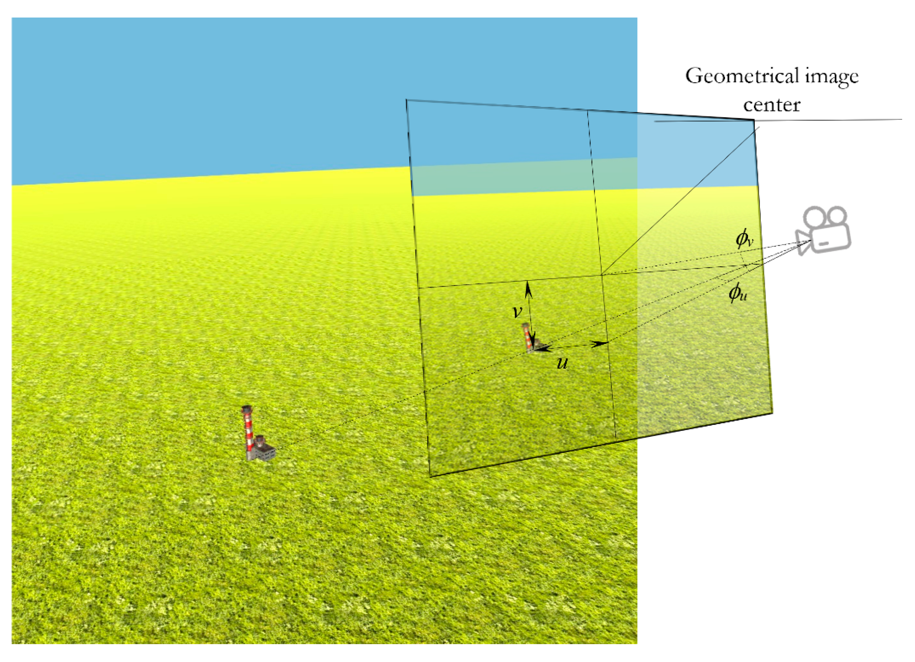
At the first stage, we use the first ANN to find coordinates u and v, describing the position of the object origin projection, on the image with reduced pixel size 227 × 227.

At the second stage, we use the second ANN to find the drone camera position and orientation ($r$—distance between camera optical center and the object origin, $W_q,X_q,Y_q,Z_q$—quaternion components, describing the camera orientation, $u_{gom}$ and $v_{gom}$—the projection point of the object origin on the modified image) using the new modified image with pixel size 227 × 227, where the object origin projection is in the image center.

3.2.1. The first Stage of Drone Camera Localization

Network Architecture and Its Training at the First Stage

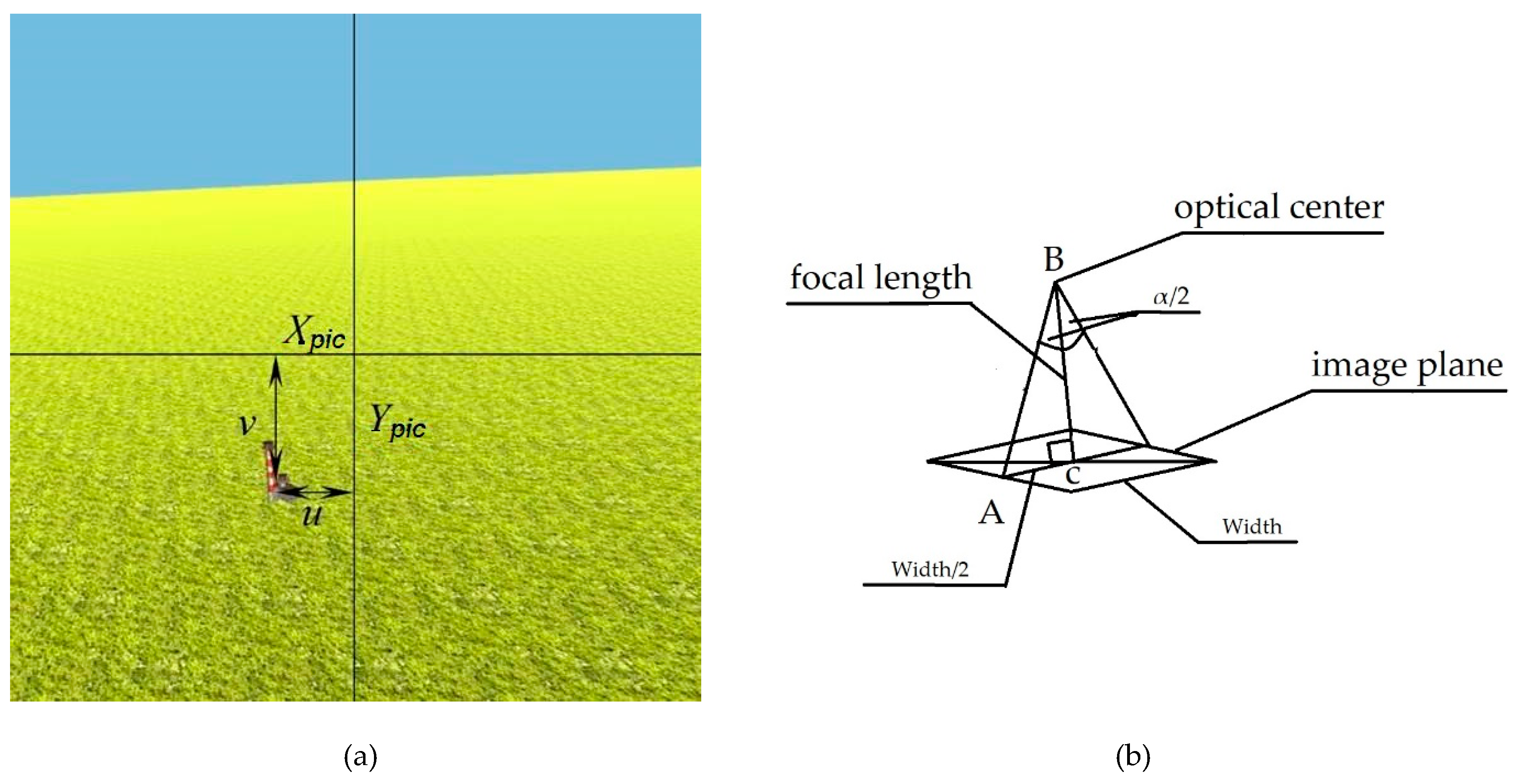
Let us describe the first stage here. We solve here the task to find the horizontal and vertical coordinates u and v of the object origin projection in a large image (Figure 4). These coordinates are equal to the pixel coordinates of the object origin projection according to the center of the image, divided by the focal length of the camera:

$$u=\frac{X_{pic}}{F}$$

(1)

$$v=\frac{Y_{pic}}{F}$$

(2)

where F is the focal length of the camera in pixels, calculated by the formula (from the right-angled triangle ABC in Figure 4b)

$$F=\frac{Width}{2}\mathrm{ctg}\left(\frac{\alpha }{2}\right),$$

(3)

where Width is the width size of the image in pixels, $\mathrm{ctg}\left(\frac{\alpha }{2}\right)=\frac{\cos \left(\frac{\alpha }{2}\right)}{\sin \left(\frac{\alpha }{2}\right)},$ and α—camera field of view in the x and y direction.

For calculation of u and v, we used the artificial neural network, which is built on the basis of AlexNet [12,13,14,15] with small changes in the structure and training method.

For our tasks, we removed the last two fully connected layers, and replaced them with one fully connected layer with 2 outputs (u and v coordinates) and one regression layer. That is, we used the pre-trained AlexNet network to solve the regression problem: determining two coordinates of the camera (Figure 5).

We reduced all images to pixel size 227 × 227 and used them for neural network training.

For training the solver, we used “adam” with 200 epochs, batch size 60, initial training velocity 0.001, and reduced the training velocity by 2 after every 20 epochs.

We have the training set (used for the artificial neural network (ANN) training) and the validation set for the verification of the pretrained ANN.

Firstly, all errors were found for the training set of images as differences between two angles (${\varphi }_u$ and ${\varphi }_v$), obtained from the pretrained artificial neural network, and the two known angles (${\varphi }_u$ and ${\varphi }_v$), used for creation of images by the Unity program. The root mean square of these errors are shown in the first row of

Table 1. Errors of coordinates u and v (for correspondent angles ${\varphi }_u$ and ${\varphi }_v$) for the object origin projection location.

Sets	σu	σv
Training set	0.0043 rad (0.24°)	0.0036 rad (0.20°)
Validation set	0.0080 rad (0.46°)	0.0070 rad (0.40°)

.

Secondly, all errors were found for the validation set of images as differences between two angles (${\varphi }_u$ and ${\varphi }_v$), obtained from the pretrained artificial neural network, and the two known angles (${\varphi }_u$ and ${\varphi }_v$), used for creation of images by the Unity program. The root mean square of these errors is shown in the second row of Table 1.

The error for finding the object origin projection coordinates u and v can be found in Table 1. Errors correspond to errors of two angles (${\varphi }_u$ and ${\varphi }_v$), as demonstrated in Figure 6.

In this way, we achieved the first-stage program purpose: to find the object origin projection position on the big image.

Homography Transformation for Translation of the Object Origin Projection to the Image Center

After finding coordinates u and v, we can accomplish homography transformation, corresponding to camera rotation on angle ${\varphi }_u$ in the horizontal direction and camera rotation on angle ${\varphi }_v$ in the vertical direction. After this transformation, the object origin projection moves to the image center (Figure 6).

Assuming that focus length is equal to 1, we find the following values for ${\varphi }_u$ and ${\varphi }_v$:

$${\cos \varphi }_u=\frac{1}{\sqrt{1+u^2}},$$

(4)

$${\sin \varphi }_u=\frac{u}{\sqrt{1+u^2}},$$

(5)

$${\cos \varphi }_v=\frac{\sqrt{1+u^2}}{\sqrt{1+u^2+v^2}},$$

(6)

$${\sin \varphi }_v=\frac{v}{\sqrt{1+u^2+v^2}}.$$

(7)

Finally, we get two rotation matrices, $R_u$ and $R_v,$ which describe the homographic transformation, H (i.e., linear transformation, moving points with homogeneous coordinates $\left(u_0, v_0,1\right)$ to the point $\left(u_1, v_1,1\right)$), in such a way that the object origin projection point $\left(u, v,1\right)$ moves to the point $\left(0,0,1\right)$ (Figure 7):

$$\left(0,0,1\right)=\left(u, v,1\right)·H,$$

(8)

$$H=R_v{R}_u,$$

(9)

where

$$R_v=\left[\begin{array}{ccc}1& 0& 0\\ 0& {\cos \varphi }_v& -{\sin \varphi }_v\\ 0& {\sin \varphi }_v& {\cos \varphi }_v\end{array}\right],$$

(10)

$$R_u=\left[\begin{array}{ccc}{\cos \varphi }_u& 0& {\sin \varphi }_u\\ 0& 1& 0\\ -{\sin \varphi }_u& 0& {\cos \varphi }_u\end{array}\right].$$

(11)

Indeed, H is the rotation matrix in system coordinates of the camera (center of coordinates O is in the optical center of the camera, axis OZ is the direction of the optical axis of the camera, OX axis is directed along width of the image, OY axis is directed along height of the image). The rotation H is composed of two rotations: the first rotation $R_v$ is defined around the OX axis on angle ${\varphi }_v, \mathrm{and}$ the second rotation $R_u$ is defined around the OY axis on angle ${\varphi }_u$ (see Figure 6).

Let us consider a neighborhood with pixel size 227 × 227 of point $\left(0, 0, 1\right)$, because after camera rotation, the object origin projection will be in this point. By application of homography to any point of this neighborhood (i.e., by multiplying the point homogeneous coordinates by $R_u^T{R}_v^T)$, we can find its correspondent point on the initial image and color values in this point.

In this way, we get a new set of images, where the optical axis is directed to the object origin and projection of this origin is in the image center (Figure 7).

3.2.2. The Second Stage of Drone Camera Localization

Finding Coordinates of the Object Origin Projection on the New Modified Images

Since $u$ and $v$ were found by the artificial neural network with some error, we can again find the real coordinates $u_{gom}$ and $v_{gom}$ of the object origin projection on the new modified image (obtained from homology), which will be used for training the artificial neural network in the second stage.

Transformation of Camera Coordinates to Quaternion Form

After several trials using different coordinate systems (Cartesian, cylindrical, spherical) and different angle representations, we chose quaternions for describing angle values, which does not result in the appearance of special points (where the same camera position and orientation correspond to several different representations).

In the case, when the camera is directed to the object origin, its position and orientation can be described by distance to the object origin $r$ and by two rotation angles of the vector, connecting the object origin and optical center of the camera: azimuthal $\phi$, zenith $\theta$, and camera rotation angle with respect to this vector—$\omega$ (Figure 8).

Respectively, we can find rotation matrices $R_{\phi }$, $R_{\theta },$ and $R_{\omega }$, and composite rotation matrix $R_{\phi \theta \omega }=R_{\omega }{R}_{\theta }{R}_{\phi }$. By transforming this matrix to quaternion form and further normalizing it, we get four coordinates, $W_q,X_q,Y_q,Z_q$ (index q is added to avoid getting the wrong $X_q, Y_q$, and $Z_q$ as Cartesian coordinates of the camera). These quaternions give a full and unambiguous description of the camera orientation in space.

The Artificial Neural Network for the Second Stage

At the second stage, we also used AlexNet with similar modifications, i.e., we removed the last two fully connected layers, and replaced them with one fully connected layer with 7 outputs ($r$—distance between camera optical center and the object origin, $W_q,X_q,Y_q,Z_q$—quaternion components, describing the camera orientation, $u_{gom}$ and $v_{gom}$—the projection point of the object origin on the modified image) and one regression layer.

Since the seven outputs of the fully connected layer have different scales ($r$ changes from 200 to 1000 m, and the rest of the values change between 0 and 1), we multiplied $W_q,X_q,Y_q,Z_q$, $u_{gom}$, and $v_{gom}$ by scale coefficient μ = 1000 for better training.

For the training solver, we used “adam” with 200 epochs, batch size 60, initial training velocity 0.001, and reduced the training velocity by 2 after every 20 epochs.

Training Results

We have the training set (used for the ANN training) and the validation set for the verification of the pretrained ANN.

Firstly, all errors were found for the training set of images as differences between positions and orientations, obtained from the pretrained artificial neural network, and known positions and orientations, used for creation of images by the Unity program. The root mean square of these errors are shown in the first row of

Table 2. Errors of coordinates and rotation angles for the drone camera.

Sets	σr	σW	σX	σY	σZ	σu_gom	σv_gom
Training set	2.0 m	2.2	2.3	2.4	2.2	1.5 pixels of image 2000 × 2000 (0.09°)	1.6 pixels of image 2000 × 2000 (0.09°)
Validation set	3.8 m	5.0	12.4	15.4	15.5	4.7 pixels of image 2000 × 2000 (0.27°)	6.6 pixels of image 2000 × 2000 (0.38°)

.

Secondly, all errors were found for the validation set of images as differences between positions and orientations, obtained from the pretrained artificial neural network, and known positions and orientations, used for creation of images by the Unity program. The root mean square of these errors are shown in the second row of Table 2.

Errors of the second stage are described in Table 2.

As a result, we get the camera coordinates in the space with precision up to 4 m and the camera orientation with precision up to 1°.

3.3. Automatic Control

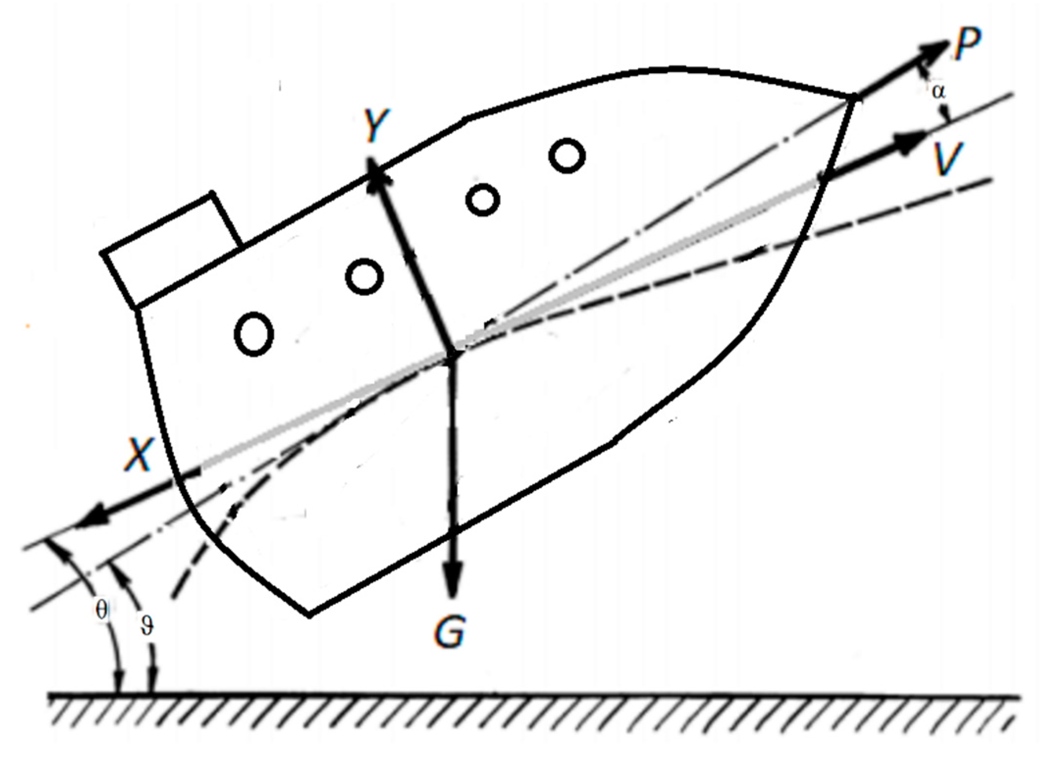
Let us define the following variables and parameters used in equations of motion for the drone (see Figure 9):

• V—Flight velocity tangent to trajectory (with respect to air)
• H—Height above mean sea level of a drone flight
• ϑ—Pitch angle, i.e., angle between longitudinal drone axis and horizontal plane
• α—Angle of attack, i.e., angle between longitudinal axis of a drone and projection of drone velocity on the symmetry plane of the drone. The drone flight is described by the system of nonlinear equations [16].

We will consider the steady-state solution as drone flight at constant velocity and height.

Let us consider small perturbation with respect to steady state:

$$\{\begin{array}{l}V=V_0+\Delta V(t)\\ \vartheta ={\vartheta }_0+\Delta \vartheta (t)\\ \alpha ={\alpha }_0+\Delta \alpha (t)\\ H=H_0+\Delta H(t)\end{array}$$

(12)

$$v\left(t\right)=\frac{\mathsf{\Delta }V}{V_0}; h\left(t\right)=\frac{\mathsf{\Delta }H}{V_0{\tau }_a}; \alpha \left(t\right)=\mathsf{\Delta }\alpha ; \vartheta \left(t\right)=\mathsf{\Delta }\vartheta ;\overline{t}=\frac{t}{{\tau }_a}$$

Linear equations for perturbations are as follows:

$$\{\begin{array}{c}{\upsilon }^{\prime }\left(t\right)=-n_{11}\upsilon \left(t\right)-n_{12}\alpha \left(t\right)-n_{13}\vartheta \left(t\right)-n_{14}h\left(t\right)=n_p{\delta }_p(t-\tau ),\\ {\alpha }^{\prime }\left(t\right)={\vartheta }^{\prime }\left(t\right)+n_{21}\upsilon \left(t\right)-n_{22}\alpha \left(t\right)+n_{23}\vartheta \left(t\right)-n_{24}h\left(t\right),\\ {\vartheta }^{″}=-n_0{\alpha }^{\prime }\left(t\right)-n_{33}{\vartheta }^{\prime }\left(t\right)-n_{31}\upsilon \left(t\right)-n_{32}\alpha \left(t\right)-n_{34}h\left(t\right)-n_B{\delta }_B(t-\tau ),\\ h^{\prime }\left(t\right)=n_{41}\upsilon \left(t\right)-n_{42}\alpha \left(t\right)+n_{42}\vartheta \left(t\right),\end{array}$$

(13)

where $v\left(t\right)$ is velocity perturbation, $h\left(t\right)$ is height perturbation, $\alpha \left(t\right)$ is attack angle perturbation, $\vartheta \left(t\right)$ is pitch angle perturbation, $\overline{t}$ is normalized by ${\tau }_a$ time t as defined above, ${\delta }_p\left(t-\tau \right)$ and ${\delta }_B\left(t-\tau \right)$ are two autopilot control parameters, and $\tau$ is time delay, which is necessary for measurement of the perturbations and calculation of the control parameters. All derivatives are made according to normalized time: $\frac{d}{d\overline{t}}.$ All $n_{ij}$ and ${\tau }_a$ are constant numerical coefficients, for which numerical values are described below.

We would like to consider some example of the flight already described previously with known constant numerical coefficients. Some typical coefficients of the linear equations (for the following flight steady-state conditions: height H₀ = 11 km, time constant ${\tau }_a=3.8 \mathrm{s},$ Mach number M = V₀/V_s = 0.9$,$ where V_s—sound velocity and V₀—drone steady-state velocity, see Table 1 from Reference [16]):

$n_{11}=0.024$, $n_{12}=-0.11$, $n_{13}=0.2$, $n_{14}=-0.00043$, $n_{21}=-0.4$, $n_{22}=2.4$, $n_{23}=0$, $n_{24}=-0.0122$, $n_{31}=0,$$n_{32}=38$, $n_{33}=2.45$, $n_{34}=-0.053$, $n_0=0.4$, $n_B=49$, $n_P=0.022$, $n_{41}=0$, $n_{42}=1$.

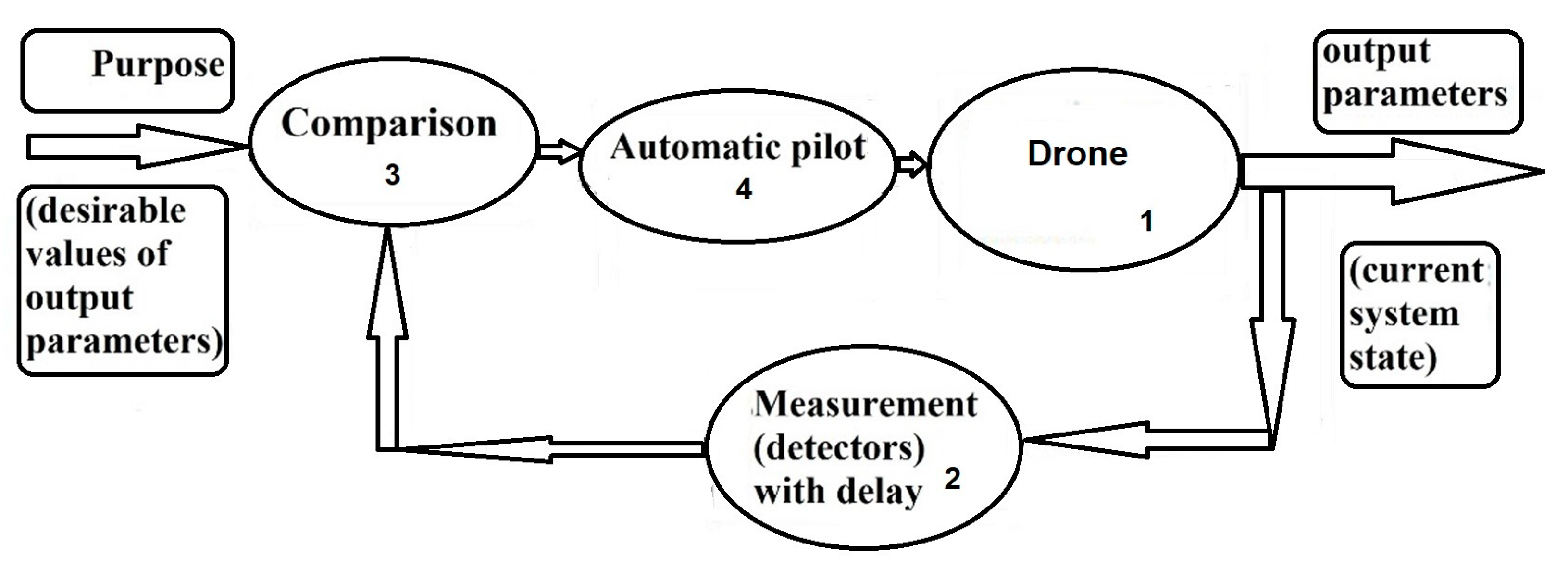
For the case when stationary parameters cannot provide stability of the desirable stationary trajectory themselves, we need to use autopilots (Figure 10). An autopilot states the control parameters, ${\delta }_p\left(t-\tau \right), {\delta }_B\left(t-\tau \right),$ to be functions of the output-controlled parameters $\left(\upsilon \left(t\right); h\left(t\right); \alpha \left(t\right); \vartheta \left(t\right)\right)$:

$${\delta }_P\left(t-\tau \right)=p_1\upsilon \left(t-\tau \right)+p_2\alpha \left(t-\tau \right)+p_3\vartheta \left(t-\tau \right)+p_{4}h\left(t-\tau \right),$$

(14)

$${\delta }_B\left(t-\tau \right)=b_1\upsilon \left(t-\tau \right)+b_2\alpha \left(t-\tau \right)+b_3\vartheta \left(t-\tau \right)+b_{4}h\left(t-\tau \right)$$

(15)

controlled parameters $\left(\upsilon \left(t\right); h\left(t\right); \alpha \left(t\right); \vartheta \left(t\right)\right)$ are perturbation with respect to the desirable stationary trajectory. The autopilot can get the output parameters from measurements of different navigation devices: from satellite navigation, inertial navigation, vision-based navigation, and so on. Using these measurements of the navigation devices, the autopilot can create controlling signals to decrease undesirable perturbations. However, any navigation measurements have some time delay $\tau$ in obtaining values of the output parameters which are controlled by autopilot. As a result, the problem exists, because some necessary information which are necessary for control does not exist.

Indeed, image processing for visual navigation demands a lot of time and results in a time delay. We can see from Figure 10 that the time delay exists in a measurement block because of a large amount of time, which is necessary for image processing of visual navigation. As a result, we know the deviation also with time delay. However, the proposed method allows to get stable control in the presence of this time delay.

In Reference [16], we demonstrate that it is possible even for such conditions with a time delay to get a controlling signal, providing a stable path.

Final solutions from Reference [16] are as follows:

We can calculate parameters $b_1, b_2, b_3, b_4$:

$$b_1=0.01142857143, b_2=-0.7559183673, b_3=0.03777242857, b_4=0.0009820408163$$

Then, we can calculate parameters $p_1$, $p_2$, $p_3$, $p_4$:

$$p_1=-35, p_2=-5.360750359, p_3=9.451659450, p_4=0.5512345678$$

The delay time is as follows:

$${\tau }_s\le 0.448{\tau }_a=0.448·3.8 \mathrm{s}=1.703 \mathrm{s}.$$

4. Conclusions

The coordinates found ($r$—distance between camera optical center and the object origin, $W_q,X_q,Y_q,Z_q$—quaternion components, describing the camera orientation, $u_{gom}$ and $v_{gom}$—the projection point of the object origin on the new modified image, $u$ and $v$—the projection points of the object origin on the initial image with reduced pixel size) unambiguously define the drone position and orientation (six degrees of freedom).

As a result, we have detailed the program which allows us unambiguously and with high precision to find the drone camera position and orientation with respect to the ground object landmark.

We can improve this result by increasing the number of images in the training set, using ANN with more complex structure, considering a more complex and more natural environment of the ground object landmark.

The errors can also be improved by changing the network configuration (like in References [7,8,9,10], for example) or by using a set of images instead of a single image [8,10].

Errors (completely describing camera position and orientation errors) were given in Table 1 and Table 2. We need not object identification error here.

We chose our ground object and background to be strongly different, so recognition quality was almost ideal. This is not because of the high quality of the deep learning network, but because of choosing an object which was very different on the background. Indeed, such a clear object is needed for robust navigation.

Image processing for visual navigation demands a lot of time and results in a time delay. We can see from Figure 10 that the time delay exists in measurement blocks because of a large amount of time, which is necessary for image processing of visual navigation. As a result, we know the deviation also with time delay. However, the proposed method allowed us to get stable control in the presence of this time delay (smaller than $1.703 \mathrm{s}$).

We have not developed real-time realization yet. So, we could not provide a description of hardware in this paper, which is necessary for real-time work. It is a topic for future research.