Figure 1.
Entire process for tests of user-based filtering.
Figure 1.
Entire process for tests of user-based filtering.
Figure 2.
Results of the prediction scores based on the Pearson correlation coefficient in the user-based filtering.
Figure 2.
Results of the prediction scores based on the Pearson correlation coefficient in the user-based filtering.
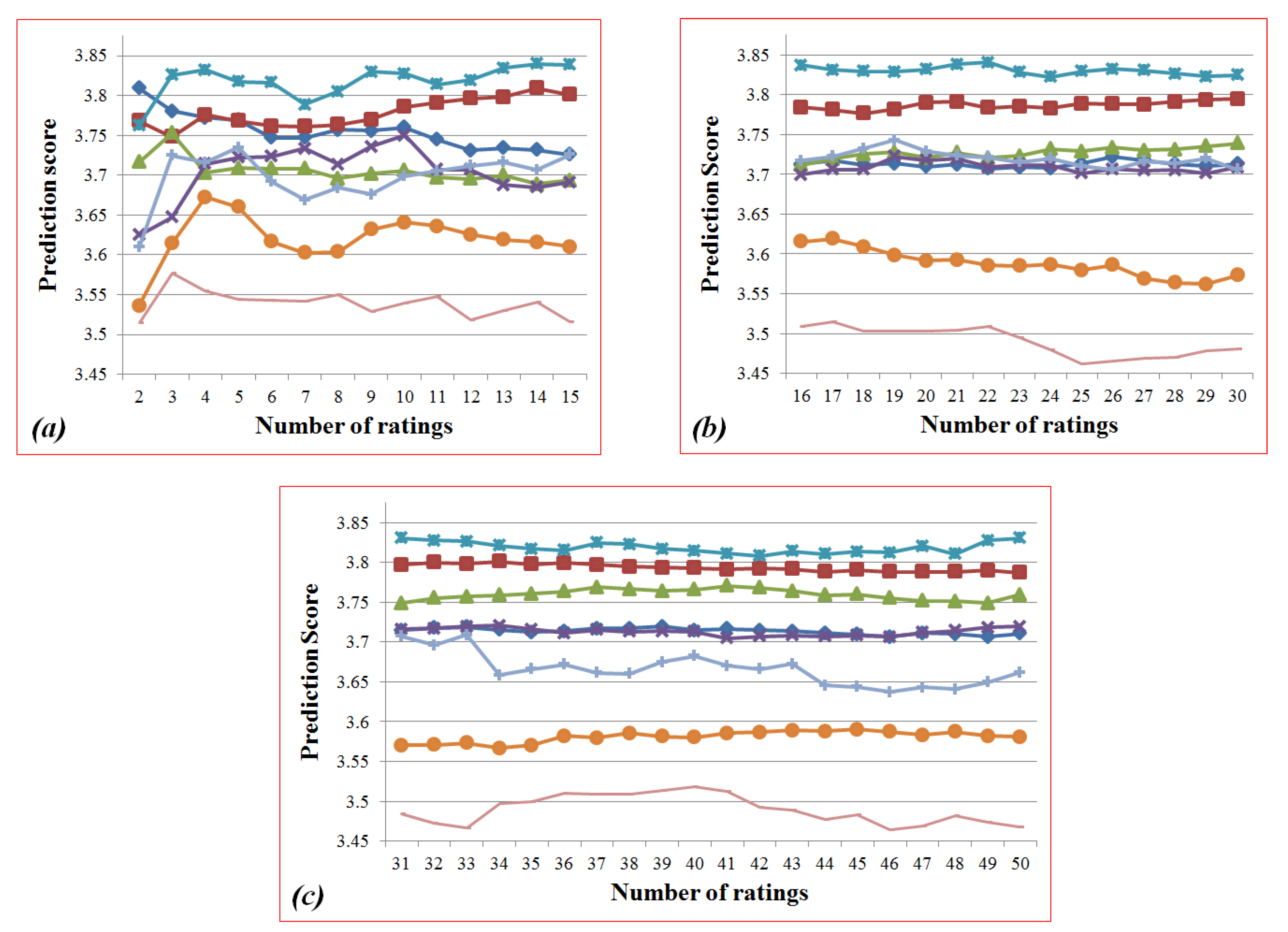
Figure 3.
Sub-graphs of
Figure 2: (
a) the ranges from 2 to 15; (
b) from 16 to 30; (
c) from 31 to 50.
Figure 3.
Sub-graphs of
Figure 2: (
a) the ranges from 2 to 15; (
b) from 16 to 30; (
c) from 31 to 50.
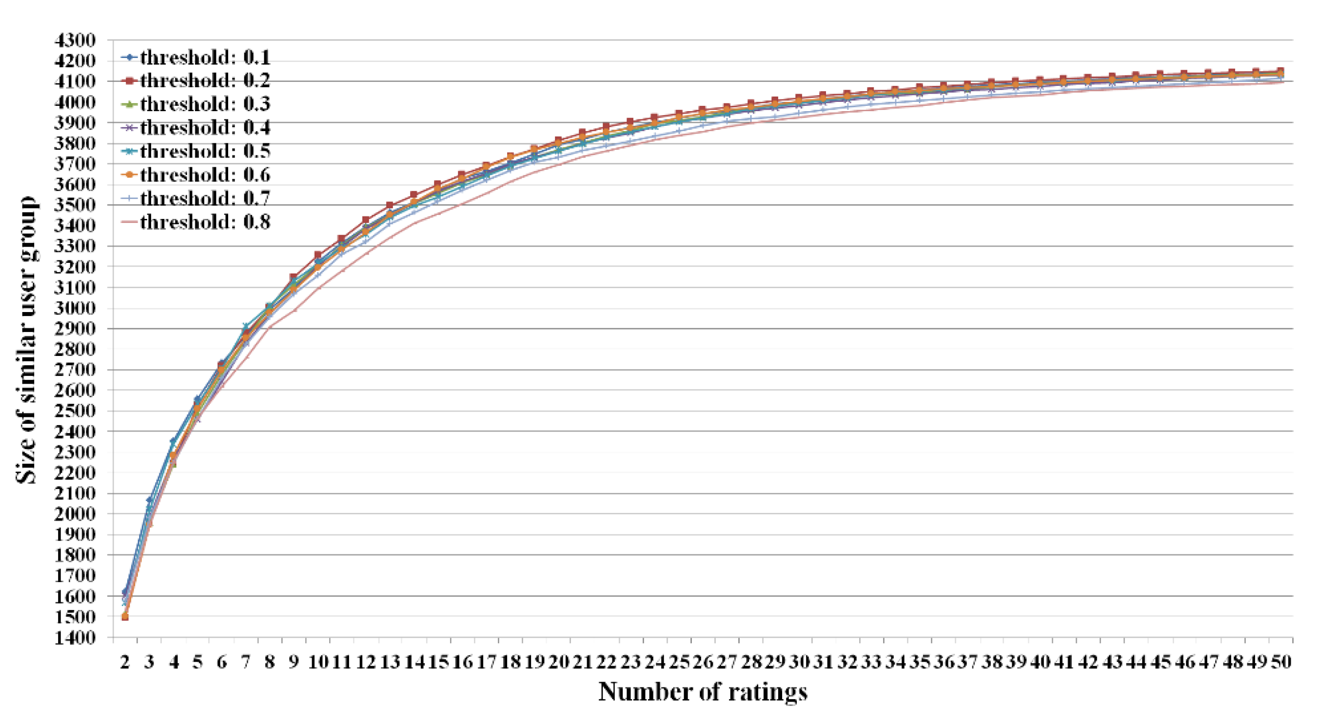
Figure 4.
Size of similar user group according to the different numbers of ratings based on the Pearson correlation coefficient.
Figure 4.
Size of similar user group according to the different numbers of ratings based on the Pearson correlation coefficient.
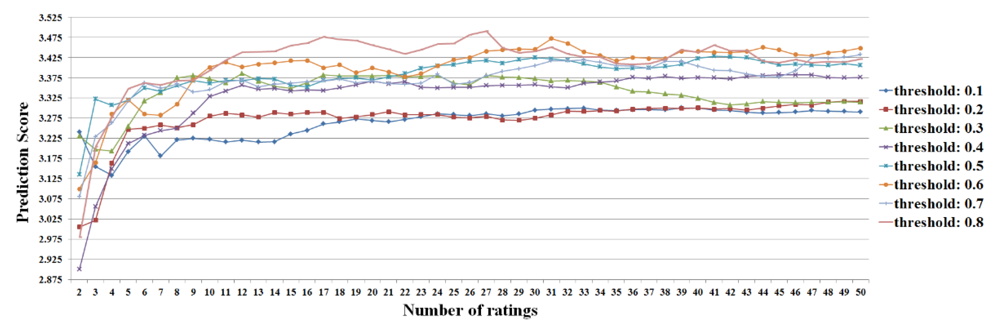
Figure 5.
Results of the prediction score based on the cosine similarity in the user-based filtering.
Figure 5.
Results of the prediction score based on the cosine similarity in the user-based filtering.
Figure 6.
Sub-graphs of
Figure 5: (
a) the ranges from 2 to 15; (
b) from 16 to 30; (
c) from 31 to 50.
Figure 6.
Sub-graphs of
Figure 5: (
a) the ranges from 2 to 15; (
b) from 16 to 30; (
c) from 31 to 50.
Figure 7.
Size of similar user group according to the different numbers of ratings based on the cosine similarity.
Figure 7.
Size of similar user group according to the different numbers of ratings based on the cosine similarity.
Figure 8.
Entire process for tests of the recommendation systems based on the item-based filtering.
Figure 8.
Entire process for tests of the recommendation systems based on the item-based filtering.
Figure 9.
Results of the prediction scores based on the Pearson correlation coefficient in the item-based filtering.
Figure 9.
Results of the prediction scores based on the Pearson correlation coefficient in the item-based filtering.
Figure 10.
Sub-graphs of
Figure 9: (
a) the ranges from 2 to 15; (
b) from 16 to 30; (
c) from 31 to 50.
Figure 10.
Sub-graphs of
Figure 9: (
a) the ranges from 2 to 15; (
b) from 16 to 30; (
c) from 31 to 50.
Figure 11.
Size of similar user group according to the different numbers of ratings based on the Pearson correlation coefficient.
Figure 11.
Size of similar user group according to the different numbers of ratings based on the Pearson correlation coefficient.
Figure 12.
Results of the prediction scores based on the cosine similarity in the item-based filtering.
Figure 12.
Results of the prediction scores based on the cosine similarity in the item-based filtering.
Figure 13.
Sub-graphs of
Figure 12: (
a) the ranges from 2 to 15; (
b) from 16 to 30; (
c) from 31 to 50.
Figure 13.
Sub-graphs of
Figure 12: (
a) the ranges from 2 to 15; (
b) from 16 to 30; (
c) from 31 to 50.
Figure 14.
Size of similar user group according to the different numbers of ratings based on the cosine similarity.
Figure 14.
Size of similar user group according to the different numbers of ratings based on the cosine similarity.
Figure 15.
Example of computing the genre frequency and frequency percentage for a user.
Figure 15.
Example of computing the genre frequency and frequency percentage for a user.
Figure 16.
Procedure example of calculating error rates.
Figure 16.
Procedure example of calculating error rates.
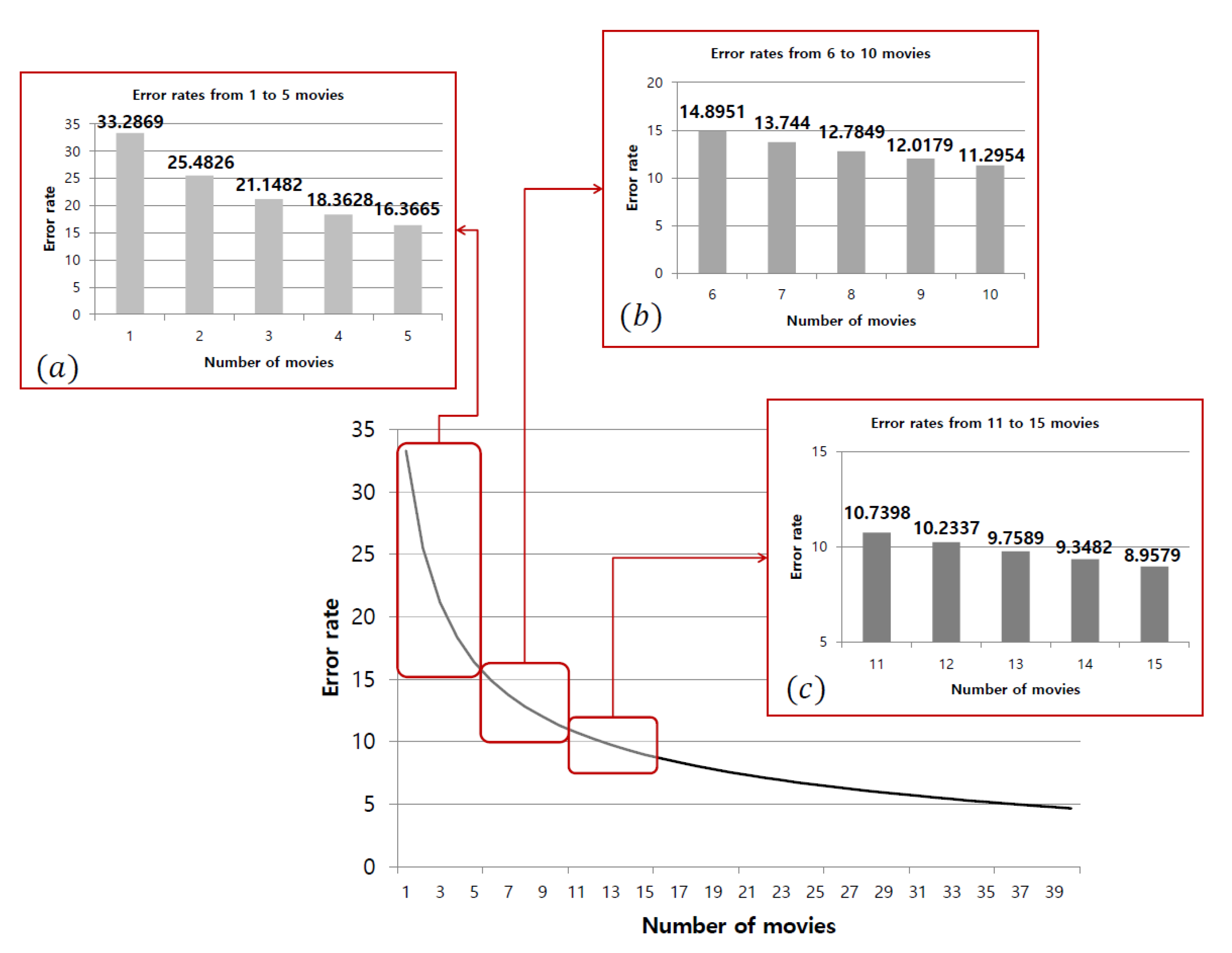
Figure 17.
Error rates for different sample sizes.
Figure 17.
Error rates for different sample sizes.
Figure 18.
Rates of decrease in error rates.
Figure 18.
Rates of decrease in error rates.
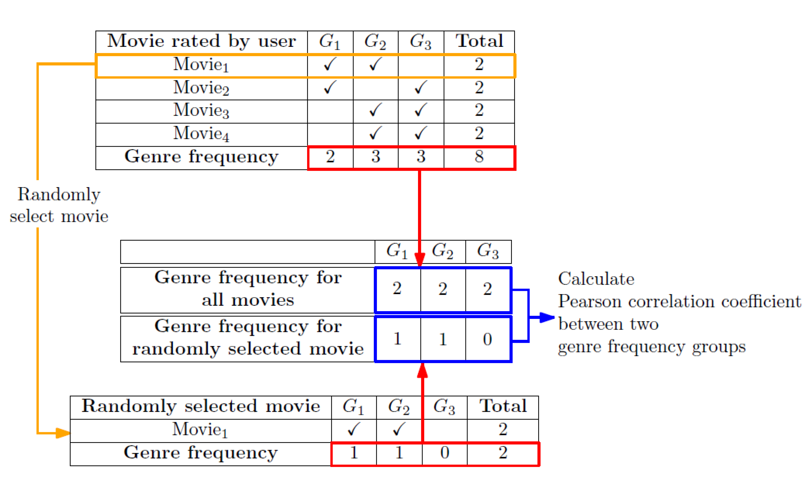
Figure 19.
Example of the procedure for calculating the Pearson correlation coefficient.
Figure 19.
Example of the procedure for calculating the Pearson correlation coefficient.
Figure 20.
Pearson correlation coefficient for different random sample sizes.
Figure 20.
Pearson correlation coefficient for different random sample sizes.
Figure 21.
Verification process of the user-based filtering.
Figure 21.
Verification process of the user-based filtering.
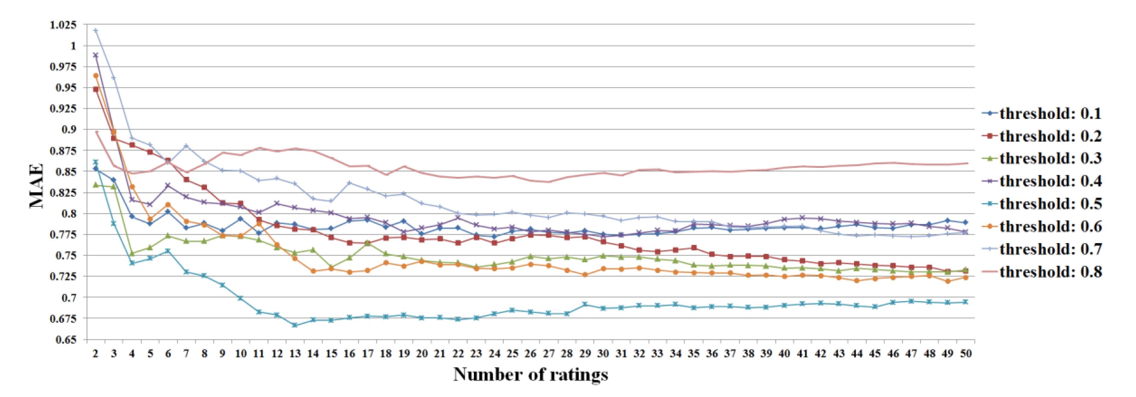
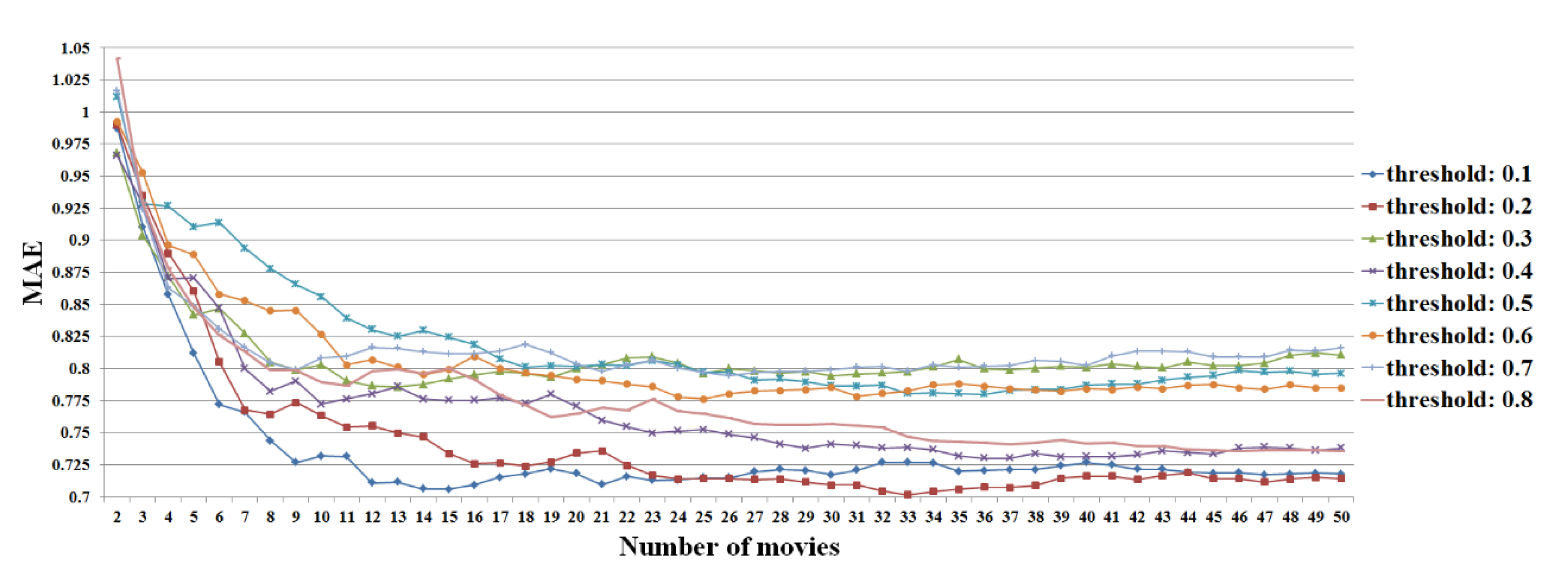
Figure 22.
Mean absolute error (MAE) values for the different numbers of ratings based on the Pearson correlation coefficient in the user-based filtering.
Figure 22.
Mean absolute error (MAE) values for the different numbers of ratings based on the Pearson correlation coefficient in the user-based filtering.
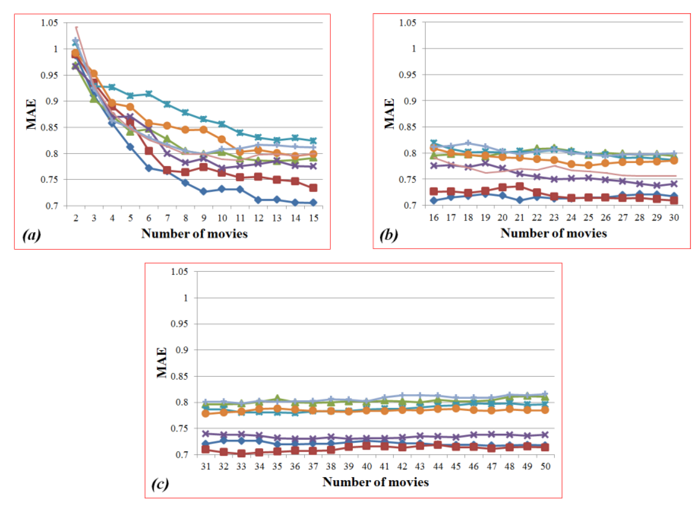
Figure 23.
Sub-graphs of
Figure 16: (
a) the ranges from 2 to 15; (
b) from 16 to 30; (
c) from 31 to 50.
Figure 23.
Sub-graphs of
Figure 16: (
a) the ranges from 2 to 15; (
b) from 16 to 30; (
c) from 31 to 50.
Figure 24.
MAE values for the different numbers of ratings based on the cosine similarity in the user-based filtering.
Figure 24.
MAE values for the different numbers of ratings based on the cosine similarity in the user-based filtering.
Figure 25.
Sub-graphs of
Figure 24: (
a) the ranges from 2 to 15; (
b) from 16 to 30; (
c) from 31 to 50.
Figure 25.
Sub-graphs of
Figure 24: (
a) the ranges from 2 to 15; (
b) from 16 to 30; (
c) from 31 to 50.
Figure 26.
Verification process of the item-based filtering.
Figure 26.
Verification process of the item-based filtering.
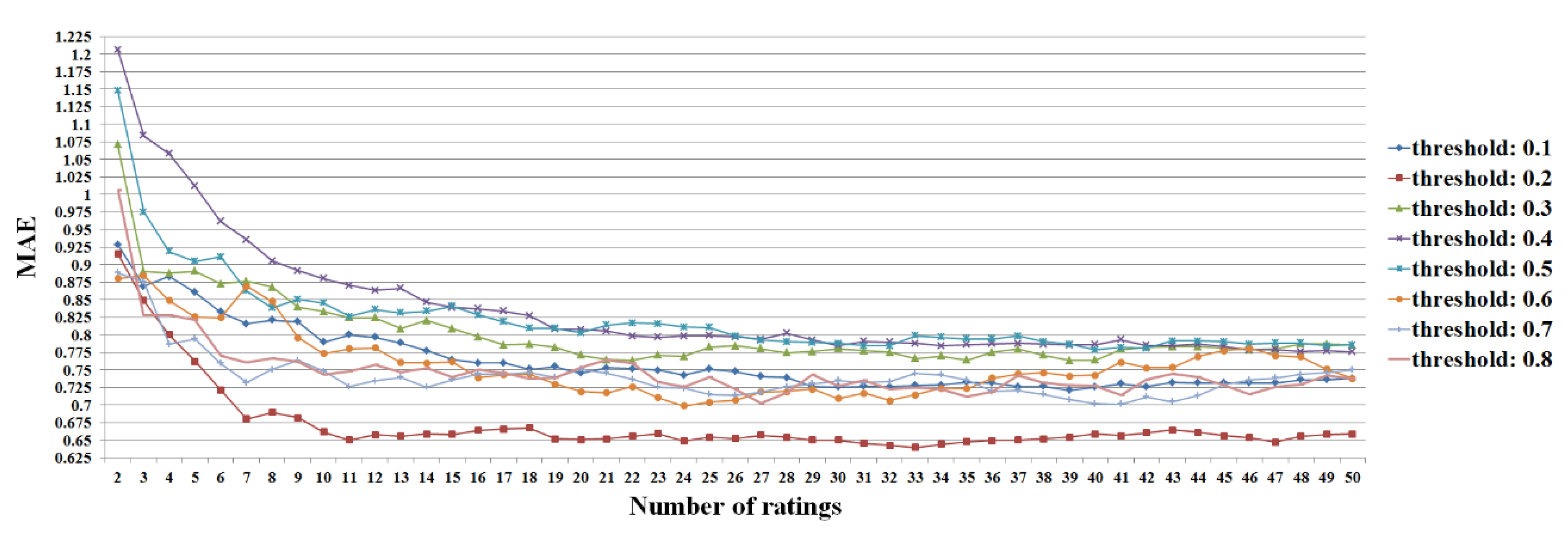
Figure 27.
MAE values for the different numbers of ratings based on the Pearson correlation coefficient in the item-based filtering.
Figure 27.
MAE values for the different numbers of ratings based on the Pearson correlation coefficient in the item-based filtering.
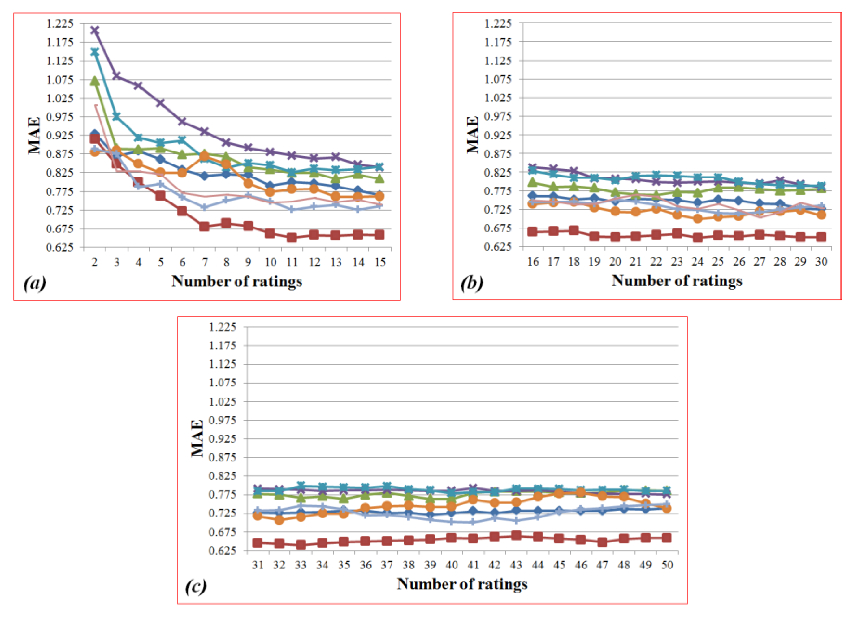
Figure 28.
Sub-graphs in
Figure 27: (
a) the ranges from 2 to 15; (
b) from 16 to 30; (
c) from 31 to 50.
Figure 28.
Sub-graphs in
Figure 27: (
a) the ranges from 2 to 15; (
b) from 16 to 30; (
c) from 31 to 50.
Figure 29.
MAE values for the different numbers of ratings based on the cosine similarity in the item-based filtering.
Figure 29.
MAE values for the different numbers of ratings based on the cosine similarity in the item-based filtering.
Figure 30.
Sub-graphs in
Figure 29: (
a) the ranges from 2 to 15; (
b) from 16 to 30; (
c) from 31 to 50.
Figure 30.
Sub-graphs in
Figure 29: (
a) the ranges from 2 to 15; (
b) from 16 to 30; (
c) from 31 to 50.
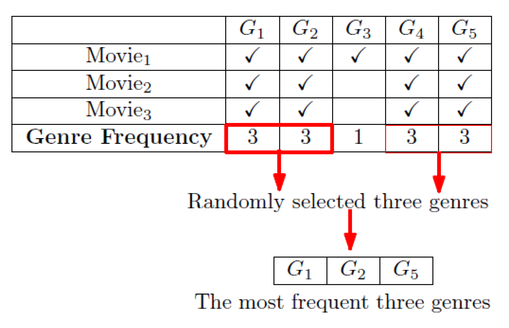
Figure 31.
Example of selecting the top three genres.
Figure 31.
Example of selecting the top three genres.
Figure 32.
Example of calculating the score using Equation (3).
Figure 32.
Example of calculating the score using Equation (3).
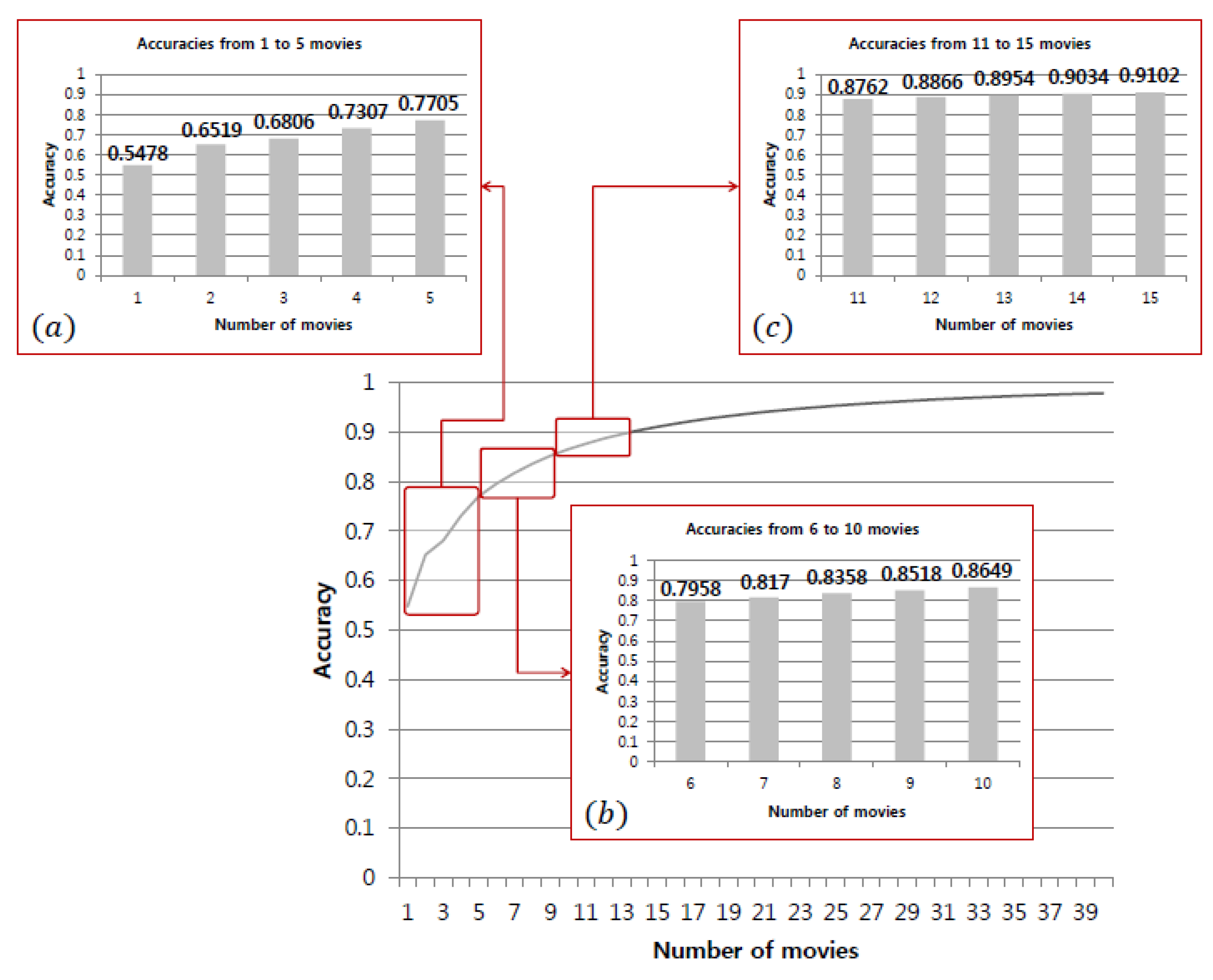
Figure 33.
Accuracy of different random sample sizes.
Figure 33.
Accuracy of different random sample sizes.
Table 1.
Number of movies that a new user has to evaluate.
Table 1.
Number of movies that a new user has to evaluate.
| Name | No. of Initial Inputs | Homepage URL |
|---|
| Jinni | 10 | [13] |
| Criticker | 10 | [14] |
| Rotten Tomatoes | 10 | [15] |
| MovieLens | 15 | [16] |
Table 2.
Studies on the cold-start problem.
Table 2.
Studies on the cold-start problem.
| Author | Year | Summary |
|---|
| Deldjoo et al. [29] | 2019 | Propose new movie recommender system that addresses the cold-start problem in the movie domain by integrating item features, exploiting an effective data fusion method |
| Tu et al. [30] | 2019 | Propose novel generative model to transfer user interests from app usage behavior to location preference and check the proposed model can reduce user-side cold-start situations |
| Jazayeriy et al. [31] | 2018 | Propose a novel similarity measure inspired by a physical resonance phenomenon, named resonance similarity, to address user cold-start problems |
| Zhang et al. [32] | 2017 | Propose a kernel-based attribute-aware matrix factorization model to address the cold-start problem for new users by utilizing the social links between users |
| Zheng et al. [33] | 2016 | Propose a tourism destination recommender system that employs opinion-mining technology to refine user preferences and item opinion reputations and embed an artificial interactive module in the proposed recommender system to alleviate the cold-start problem |
| Xu et al. [34] | 2016 | Propose a novel rating comparison strategy (RAPARE) to learn the latent profiles of cold-start users/items to break the barrier for cold-start users/items |
| Xu et al. [35] | 2015 | Propose a novel rating comparison strategy to break user/item cold-start situations |
| Gogna et al. [36] | 2015 | Enhance prediction accuracy in cold-start situations of the recommender systems, propose a method that utilizes secondary information such as user’s demography and item categories |
| Lika et al. [24] | 2014 | Propose a classification method for demographic data and calculate user similarity. |
| Bobadilla et al. [37] | 2012 | Suggest a metric criterion of similarity between new users based on neural learning. The proposed similarity metric criterion provides more precise results than a previous metric criterion. |
| Zhang et al. [25] | 2010 | Alleviate user-side cold-start problems using collaborative tagging systems. |
| Lam et al. [19] | 2008 | Report a hybrid method that alleviates the user-side cold-start problem through user and item attributes such as year, age and gender. |
Table 3.
GroupLens movie database.
Table 3.
GroupLens movie database.
| Dataset | Attribute | 1 M Size | 10 M Size |
|---|
| Movie Dataset | MovieID, Title, Genre | 3900 movies | 10,681 movies |
| User Dataset | UserID, Gender, Age, Occupation, ZIP-code | 6040 users | 69,898 users |
| Rating Dataset | UserID, MovieID, Rating, Timestamp | 1,000,209 ratings | 10,000,054 ratings |
Table 4.
The 18 genres in the GroupLens database.
Table 4.
The 18 genres in the GroupLens database.
| No | Genre | No | Genre | No | Genre |
|---|
| G1 | Action | G7 | Documentary | G13 | Mystery |
| G2 | Adventure | G9 | Drama | G14 | Romance |
| G3 | Animation | G9 | Fantasy | G15 | Sci-Fi |
| G4 | Children’s | G10 | Film-Noir | G16 | Thriller |
| G5 | Comedy | G11 | Horror | G17 | War |
| G6 | Crime | G12 | Musical | G18 | Western |
Table 5.
Changing average of prediction and difference for each range (the user-based filtering: the Pearson correlation coefficient).
Table 5.
Changing average of prediction and difference for each range (the user-based filtering: the Pearson correlation coefficient).
| Input Size | Average Predictions | Difference | No. | Average Predictions | Difference |
|---|
| 2 | 3.6676 | - | 27 | 3.6906 | 0.0016 |
| 3 | 3.7087 | 0.0411 | 28 | 3.6893 | 0.0013 |
| 4 | 3.7175 | 0.0088 | 29 | 3.6904 | 0.0011 |
| 5 | 3.7156 | 0.0019 | 30 | 3.6924 | 0.0020 |
| 6 | 3.7010 | 0.0146 | 31 | 3.6959 | 0.0035 |
| 7 | 3.6940 | 0.0070 | 32 | 3.6946 | 0.0013 |
| 8 | 3.6965 | 0.0026 | 33 | 3.6960 | 0.0013 |
| 9 | 3.7038 | 0.0073 | 34 | 3.6924 | 0.0036 |
| 10 | 3.7134 | 0.0096 | 35 | 3.6923 | 0.0001 |
| 11 | 3.7053 | 0.0081 | 36 | 3.6957 | 0.0034 |
| 12 | 3.7006 | 0.0048 | 37 | 3.6964 | 0.0007 |
| 13 | 3.7025 | 0.0019 | 38 | 3.6960 | 0.0004 |
| 14 | 3.7021 | 0.0004 | 39 | 3.6971 | 0.0011 |
| 15 | 3.7001 | 0.0019 | 40 | 3.6978 | 0.0006 |
| 16 | 3.6982 | 0.0019 | 41 | 3.6951 | 0.0027 |
| 17 | 3.7014 | 0.0032 | 42 | 3.6918 | 0.0032 |
| 18 | 3.6991 | 0.0023 | 43 | 3.6927 | 0.0008 |
| 19 | 3.7022 | 0.0031 | 44 | 3.6856 | 0.0070 |
| 20 | 3.6991 | 0.0031 | 45 | 3.6873 | 0.0017 |
| 21 | 3.7010 | 0.0019 | 46 | 3.6822 | 0.0051 |
| 22 | 3.6969 | 0.0041 | 47 | 3.6847 | 0.0025 |
| 23 | 3.6940 | 0.0029 | 48 | 3.6854 | 0.0007 |
| 24 | 3.6927 | 0.0013 | 49 | 3.6871 | 0.0016 |
| 25 | 3.6891 | 0.0036 | 50 | 3.6896 | 0.0025 |
| 26 | 3.6923 | 0.0032 | | | |
Table 6.
Changing average of prediction and difference for each range (the user-based filtering: the cosine similarity).
Table 6.
Changing average of prediction and difference for each range (the user-based filtering: the cosine similarity).
| Input Size | Average Predictions | Difference | No. | Average Predictions | Difference |
|---|
| 2 | 3.7542 | - | 27 | 3.7241 | 0.0008 |
| 3 | 3.7373 | 0.0169 | 28 | 3.7268 | 0.0027 |
| 4 | 3.7335 | 0.0038 | 29 | 3.7262 | 0.0006 |
| 5 | 3.7231 | 0.0104 | 30 | 3.7278 | 0.0016 |
| 6 | 3.7137 | 0.0094 | 31 | 3.7258 | 0.0020 |
| 7 | 3.7238 | 0.0101 | 32 | 3.7239 | 0.0019 |
| 8 | 3.7195 | 0.0044 | 33 | 3.7235 | 0.0004 |
| 9 | 3.7227 | 0.0032 | 34 | 3.7227 | 0.0007 |
| 10 | 3.7225 | 0.0001 | 35 | 3.7238 | 0.0010 |
| 11 | 3.7266 | 0.0040 | 36 | 3.7232 | 0.0006 |
| 12 | 3.7202 | 0.0064 | 37 | 3.7244 | 0.0012 |
| 13 | 3.7162 | 0.0040 | 38 | 3.7243 | 0.0001 |
| 14 | 3.7160 | 0.0002 | 39 | 3.7248 | 0.0005 |
| 15 | 3.7113 | 0.0048 | 40 | 3.7269 | 0.0021 |
| 16 | 3.7083 | 0.0030 | 41 | 3.7269 | 0.0000 |
| 17 | 3.7117 | 0.0034 | 42 | 3.7246 | 0.0022 |
| 18 | 3.7108 | 0.0009 | 43 | 3.7231 | 0.0016 |
| 19 | 3.7095 | 0.0012 | 44 | 3.7234 | 0.0003 |
| 20 | 3.7124 | 0.0029 | 45 | 3.7227 | 0.0007 |
| 21 | 3.7135 | 0.0011 | 46 | 3.7235 | 0.0008 |
| 22 | 3.7154 | 0.0019 | 47 | 3.7240 | 0.0004 |
| 23 | 3.7150 | 0.0003 | 48 | 3.7225 | 0.0015 |
| 24 | 3.7215 | 0.0065 | 49 | 3.7217 | 0.0007 |
| 25 | 3.7241 | 0.0026 | 50 | 3.7230 | 0.0013 |
| 26 | 3.7250 | 0.0009 | | | |
Table 7.
Changing average of prediction and difference for each range (the item-based filtering: the Pearson correlation coefficient).
Table 7.
Changing average of prediction and difference for each range (the item-based filtering: the Pearson correlation coefficient).
| Input Size | Average Predictions | Difference | No. | Average Predictions | Difference |
|---|
| 2 | 3.0839 | - | 27 | 3.3790 | 0.0098 |
| 3 | 3.1687 | 0.0848 | 28 | 3.3727 | 0.0063 |
| 4 | 3.2214 | 0.0527 | 29 | 3.3733 | 0.0006 |
| 5 | 3.2765 | 0.0551 | 30 | 3.3772 | 0.0038 |
| 6 | 3.2989 | 0.0224 | 31 | 3.3828 | 0.0057 |
| 7 | 3.2941 | 0.0048 | 32 | 3.3802 | 0.0027 |
| 8 | 3.3112 | 0.0171 | 33 | 3.3769 | 0.0033 |
| 9 | 3.3249 | 0.0136 | 34 | 3.3739 | 0.0030 |
| 10 | 3.3382 | 0.0133 | 35 | 3.3671 | 0.0068 |
| 11 | 3.3467 | 0.0086 | 36 | 3.3686 | 0.0015 |
| 12 | 3.3531 | 0.0063 | 37 | 3.3676 | 0.0010 |
| 13 | 3.3477 | 0.0053 | 38 | 3.3717 | 0.0040 |
| 14 | 3.3489 | 0.0012 | 39 | 3.3769 | 0.0053 |
| 15 | 3.3503 | 0.0014 | 40 | 3.3758 | 0.0011 |
| 16 | 3.3548 | 0.0045 | 41 | 3.3749 | 0.0009 |
| 17 | 3.3612 | 0.0064 | 42 | 3.3716 | 0.0033 |
| 18 | 3.3617 | 0.0005 | 43 | 3.3707 | 0.0009 |
| 19 | 3.3602 | 0.0015 | 44 | 3.3683 | 0.0023 |
| 20 | 3.3614 | 0.0012 | 45 | 3.3668 | 0.0016 |
| 21 | 3.3591 | 0.0023 | 46 | 3.3686 | 0.0019 |
| 22 | 3.3568 | 0.0023 | 47 | 3.3716 | 0.0030 |
| 23 | 3.3603 | 0.0035 | 48 | 3.3725 | 0.0008 |
| 24 | 3.3691 | 0.0089 | 49 | 3.3738 | 0.0013 |
| 25 | 3.3650 | 0.0041 | 50 | 3.3759 | 0.0021 |
| 26 | 3.3692 | 0.0042 | | | |
Table 8.
Changing average of prediction and difference for each range (the item-based filtering: the cosine similarity).
Table 8.
Changing average of prediction and difference for each range (the item-based filtering: the cosine similarity).
| Input Size | Average Predictions | Difference | No. | Average Predictions | Difference |
|---|
| 2 | 3.1261 | - | 27 | 3.3332 | 0.0013 |
| 3 | 3.1681 | 0.0420 | 28 | 3.3334 | 0.0003 |
| 4 | 3.2150 | 0.0469 | 29 | 3.3337 | 0.0003 |
| 5 | 3.2598 | 0.0449 | 30 | 3.3356 | 0.0018 |
| 6 | 3.2804 | 0.0206 | 31 | 3.3354 | 0.0002 |
| 7 | 3.2915 | 0.0111 | 32 | 3.3346 | 0.0008 |
| 8 | 3.3090 | 0.0174 | 33 | 3.3342 | 0.0004 |
| 9 | 3.3168 | 0.0078 | 34 | 3.3335 | 0.0007 |
| 10 | 3.3191 | 0.0024 | 35 | 3.3321 | 0.0014 |
| 11 | 3.3222 | 0.0030 | 36 | 3.3329 | 0.0009 |
| 12 | 3.3247 | 0.0025 | 37 | 3.3333 | 0.0004 |
| 13 | 3.3244 | 0.0003 | 38 | 3.3335 | 0.0002 |
| 14 | 3.3273 | 0.0029 | 39 | 3.3322 | 0.0013 |
| 15 | 3.3319 | 0.0046 | 40 | 3.3311 | 0.0011 |
| 16 | 3.3351 | 0.0032 | 41 | 3.3306 | 0.0005 |
| 17 | 3.3325 | 0.0026 | 42 | 3.3289 | 0.0017 |
| 18 | 3.3317 | 0.0008 | 43 | 3.3290 | 0.0001 |
| 19 | 3.3315 | 0.0002 | 44 | 3.3304 | 0.0013 |
| 20 | 3.3328 | 0.0014 | 45 | 3.3308 | 0.0005 |
| 21 | 3.3344 | 0.0016 | 46 | 3.3309 | 0.0001 |
| 22 | 3.3348 | 0.0004 | 47 | 3.3321 | 0.0012 |
| 23 | 3.3350 | 0.0002 | 48 | 3.3334 | 0.0013 |
| 24 | 3.3325 | 0.0025 | 49 | 3.3335 | 0.0001 |
| 25 | 3.3297 | 0.0028 | 50 | 3.3341 | 0.0006 |
| 26 | 3.3319 | 0.0022 | | | |
Table 9.
Correlation coefficients for each random sample size.
Table 9.
Correlation coefficients for each random sample size.
| No. | Corr. | No. | Corr. | No. | Corr. | No. | Corr. |
|---|
| 1 | 0.4311 | 11 | 0.8485 | 21 | 0.9186 | 31 | 0.9487 |
| 2 | 0.5527 | 12 | 0.8605 | 22 | 0.9232 | 32 | 0.9507 |
| 3 | 0.6305 | 13 | 0.8701 | 23 | 0.9269 | 33 | 0.9527 |
| 4 | 0.6833 | 14 | 0.8778 | 24 | 0.9304 | 34 | 0.9543 |
| 5 | 0.7263 | 15 | 0.8862 | 25 | 0.9334 | 35 | 0.9560 |
| 6 | 0.7565 | 16 | 0.8929 | 26 | 0.9391 | 36 | 0.9576 |
| 7 | 0.7830 | 17 | 0.8995 | 27 | 0.9391 | 37 | 0.9592 |
| 8 | 0.8027 | 18 | 0.9053 | 28 | 0.9417 | 38 | 0.9607 |
| 9 | 0.8206 | 19 | 0.9102 | 29 | 0.9440 | 39 | 0.9623 |
| 10 | 0.8359 | 20 | 0.9144 | 30 | 0.9460 | 40 | 0.9636 |
Table 10.
Change in the average of MAE and average difference for each range (the user-based filtering: the Pearson correlation coefficient).
Table 10.
Change in the average of MAE and average difference for each range (the user-based filtering: the Pearson correlation coefficient).
| Input Size | Average MAE | Difference | No. | Average MAE | Difference |
|---|
| 2 | 0.9852 | - | 27 | 0.7893 | 0.0018 |
| 3 | 0.9298 | 0.0554 | 28 | 0.7893 | 0.0000 |
| 4 | 0.8909 | 0.0389 | 29 | 0.7871 | 0.0021 |
| 5 | 0.8580 | 0.0329 | 30 | 0.7864 | 0.0007 |
| 6 | 0.8401 | 0.0179 | 31 | 0.7862 | 0.0003 |
| 7 | 0.8354 | 0.0047 | 32 | 0.7846 | 0.0016 |
| 8 | 0.8245 | 0.0109 | 33 | 0.7893 | 0.0047 |
| 9 | 0.8222 | 0.0024 | 34 | 0.7880 | 0.0013 |
| 10 | 0.8178 | 0.0044 | 35 | 0.7870 | 0.0010 |
| 11 | 0.8147 | 0.0031 | 36 | 0.7883 | 0.0013 |
| 12 | 0.8045 | 0.0102 | 37 | 0.7898 | 0.0014 |
| 13 | 0.7996 | 0.0049 | 38 | 0.7882 | 0.0016 |
| 14 | 0.7994 | 0.0002 | 39 | 0.7923 | 0.0041 |
| 15 | 0.8020 | 0.0025 | 40 | 0.7958 | 0.0035 |
| 16 | 0.7976 | 0.0044 | 41 | 0.7941 | 0.0017 |
| 17 | 0.7975 | 0.0001 | 42 | 0.7938 | 0.0003 |
| 18 | 0.7979 | 0.0004 | 43 | 0.7926 | 0.0012 |
| 19 | 0.7929 | 0.0049 | 44 | 0.7935 | 0.0009 |
| 20 | 0.7912 | 0.0018 | 45 | 0.7921 | 0.0014 |
| 21 | 0.7917 | 0.0005 | 46 | 0.7945 | 0.0024 |
| 22 | 0.7919 | 0.0002 | 47 | 0.7963 | 0.0019 |
| 23 | 0.7905 | 0.0014 | 48 | 0.7953 | 0.0010 |
| 24 | 0.7937 | 0.0033 | 49 | 0.7968 | 0.0015 |
| 25 | 0.7897 | 0.0041 | 50 | 0.7952 | 0.0017 |
| 26 | 0.7911 | 0.0015 | | | |
Table 11.
Change in the average of MAE and average difference for each range (the user-based filtering: the cosine similarity).
Table 11.
Change in the average of MAE and average difference for each range (the user-based filtering: the cosine similarity).
| Input Size | Average MAE | Difference | No. | Average MAE | Difference |
|---|
| 2 | 0.9204 | - | 27 | 0.7661 | 0.0015 |
| 3 | 0.8700 | 0.0504 | 28 | 0.7662 | 0.0001 |
| 4 | 0.8195 | 0.0505 | 29 | 0.7670 | 0.0007 |
| 5 | 0.8127 | 0.0068 | 30 | 0.7662 | 0.0008 |
| 6 | 0.8198 | 0.0071 | 31 | 0.7645 | 0.0017 |
| 7 | 0.8075 | 0.0123 | 32 | 0.7661 | 0.0015 |
| 8 | 0.8041 | 0.0034 | 33 | 0.7658 | 0.0003 |
| 9 | 0.7987 | 0.0055 | 34 | 0.7649 | 0.0009 |
| 10 | 0.7972 | 0.0015 | 35 | 0.7655 | 0.0006 |
| 11 | 0.7909 | 0.0063 | 36 | 0.7646 | 0.0009 |
| 12 | 0.7878 | 0.0031 | 37 | 0.7631 | 0.0015 |
| 13 | 0.7818 | 0.0060 | 38 | 0.7627 | 0.0003 |
| 14 | 0.7772 | 0.0046 | 39 | 0.7635 | 0.0007 |
| 15 | 0.7722 | 0.0051 | 40 | 0.7637 | 0.0002 |
| 16 | 0.7745 | 0.0023 | 41 | 0.7646 | 0.0009 |
| 17 | 0.7765 | 0.0020 | 42 | 0.7629 | 0.0017 |
| 18 | 0.7726 | 0.0039 | 43 | 0.7620 | 0.0009 |
| 19 | 0.7730 | 0.0004 | 44 | 0.7614 | 0.0006 |
| 20 | 0.7686 | 0.0044 | 45 | 0.7609 | 0.0005 |
| 21 | 0.7683 | 0.0003 | 46 | 0.7613 | 0.0004 |
| 22 | 0.7673 | 0.0010 | 47 | 0.7616 | 0.0002 |
| 23 | 0.7650 | 0.0023 | 48 | 0.7612 | 0.0003 |
| 24 | 0.7642 | 0.0008 | 49 | 0.7604 | 0.0008 |
| 25 | 0.7676 | 0.0034 | 50 | 0.7607 | 0.0003 |
| 26 | 0.7676 | 0.0000 | | | |
Table 12.
Change in the average of MAE and difference for each range (the item-based filtering: the Pearson correlation coefficient).
Table 12.
Change in the average of MAE and difference for each range (the item-based filtering: the Pearson correlation coefficient).
| Input Size | Average MAE | Difference | No. | Average MAE | Difference |
|---|
| 2 | 1.0058 | - | 27 | 0.7382 | 0.0025 |
| 3 | 0.9072 | 0.0986 | 28 | 0.7406 | 0.0024 |
| 4 | 0.8766 | 0.0306 | 29 | 0.7414 | 0.0008 |
| 5 | 0.8590 | 0.0177 | 30 | 0.7377 | 0.0037 |
| 6 | 0.8320 | 0.0270 | 31 | 0.7388 | 0.0012 |
| 7 | 0.8167 | 0.0152 | 32 | 0.7351 | 0.0038 |
| 8 | 0.8110 | 0.0057 | 33 | 0.7384 | 0.0034 |
| 9 | 0.8006 | 0.0104 | 34 | 0.7394 | 0.0009 |
| 10 | 0.7847 | 0.0159 | 35 | 0.7372 | 0.0022 |
| 11 | 0.7783 | 0.0063 | 36 | 0.7396 | 0.0024 |
| 12 | 0.7816 | 0.0032 | 37 | 0.7439 | 0.0043 |
| 13 | 0.7750 | 0.0066 | 38 | 0.7402 | 0.0037 |
| 14 | 0.7720 | 0.0029 | 39 | 0.7364 | 0.0038 |
| 15 | 0.7688 | 0.0033 | 40 | 0.7358 | 0.0006 |
| 16 | 0.7653 | 0.0035 | 41 | 0.7399 | 0.0041 |
| 17 | 0.7622 | 0.0031 | 42 | 0.7422 | 0.0023 |
| 18 | 0.7589 | 0.0033 | 43 | 0.7452 | 0.0030 |
| 19 | 0.7520 | 0.0069 | 44 | 0.7473 | 0.0021 |
| 20 | 0.7504 | 0.0016 | 45 | 0.7474 | 0.0001 |
| 21 | 0.7522 | 0.0018 | 46 | 0.7454 | 0.0020 |
| 22 | 0.7514 | 0.0008 | 47 | 0.7454 | 0.0001 |
| 23 | 0.7453 | 0.0061 | 48 | 0.7485 | 0.0031 |
| 24 | 0.7401 | 0.0051 | 49 | 0.7479 | 0.0006 |
| 25 | 0.7448 | 0.0047 | 50 | 0.7464 | 0.0015 |
| 26 | 0.7407 | 0.0041 | | | |
Table 13.
Change in the average MAE and average difference for each range (the item-based filtering: the cosine similarity).
Table 13.
Change in the average MAE and average difference for each range (the item-based filtering: the cosine similarity).
| Input Size | Average MAE | Difference | No. | Average MAE | Difference |
|---|
| 2 | 0.9968 | - | 27 | 0.7631 | 0.0007 |
| 3 | 0.9265 | 0.0703 | 28 | 0.7627 | 0.0004 |
| 4 | 0.8816 | 0.0448 | 29 | 0.7618 | 0.0009 |
| 5 | 0.8599 | 0.0217 | 30 | 0.7611 | 0.0007 |
| 6 | 0.8374 | 0.0226 | 31 | 0.7609 | 0.0002 |
| 7 | 0.8172 | 0.0202 | 32 | 0.7611 | 0.0002 |
| 8 | 0.8027 | 0.0145 | 33 | 0.7590 | 0.0021 |
| 9 | 0.7998 | 0.0029 | 34 | 0.7603 | 0.0013 |
| 10 | 0.7937 | 0.0060 | 35 | 0.7596 | 0.0008 |
| 11 | 0.7863 | 0.0074 | 36 | 0.7585 | 0.0011 |
| 12 | 0.7856 | 0.0007 | 37 | 0.7584 | 0.0001 |
| 13 | 0.7842 | 0.0014 | 38 | 0.7598 | 0.0014 |
| 14 | 0.7814 | 0.0029 | 39 | 0.7608 | 0.0010 |
| 15 | 0.7802 | 0.0012 | 40 | 0.7613 | 0.0005 |
| 16 | 0.7795 | 0.0007 | 41 | 0.7624 | 0.0011 |
| 17 | 0.7771 | 0.0024 | 42 | 0.7619 | 0.0004 |
| 18 | 0.7748 | 0.0023 | 43 | 0.7628 | 0.0009 |
| 19 | 0.7742 | 0.0007 | 44 | 0.7634 | 0.0006 |
| 20 | 0.7730 | 0.0012 | 45 | 0.7620 | 0.0014 |
| 21 | 0.7711 | 0.0019 | 46 | 0.7626 | 0.0006 |
| 22 | 0.7705 | 0.0007 | 47 | 0.7623 | 0.0003 |
| 23 | 0.7703 | 0.0001 | 48 | 0.7645 | 0.0022 |
| 24 | 0.7662 | 0.0041 | 49 | 0.7641 | 0.0004 |
| 25 | 0.7641 | 0.0021 | 50 | 0.7641 | 0.0000 |
| 26 | 0.7638 | 0.0003 | | | |
Table 14.
Accuracy change and average difference for each range.
Table 14.
Accuracy change and average difference for each range.
| No. | Accuracy | Difference | No. | Accuracy | Difference |
|---|
| 1 | 0.5478 | - | 21 | 0.9403 | 0.0041 |
| 2 | 0.6517 | 0.1041 | 22 | 0.9437 | 0.0034 |
| 3 | 0.6806 | 0.0287 | 23 | 0.9470 | 0.0033 |
| 4 | 0.7307 | 0.0501 | 24 | 0.9500 | 0.0030 |
| 5 | 0.7705 | 0.0399 | 25 | 0.9529 | 0.0029 |
| 6 | 0.7958 | 0.0253 | 26 | 0.9554 | 0.0024 |
| 7 | 0.8170 | 0.0213 | 27 | 0.9579 | 0.0025 |
| 8 | 0.8358 | 0.0188 | 28 | 0.9600 | 0.0021 |
| 9 | 0.8518 | 0.0159 | 29 | 0.9623 | 0.0023 |
| 10 | 0.8649 | 0.0132 | 30 | 0.9644 | 0.0021 |
| 11 | 08762 | 0.0113 | 31 | 0.9662 | 0.0018 |
| 12 | 0.8866 | 0.0104 | 32 | 0.9678 | 0.0016 |
| 13 | 0.8954 | 0.0088 | 33 | 0.9694 | 0.0016 |
| 14 | 0.9034 | 0.0080 | 34 | 0.9710 | 0.0016 |
| 15 | 0.9102 | 0.0068 | 35 | 0.9724 | 0.0014 |
| 16 | 0.9164 | 0.0062 | 36 | 0.9738 | 0.0014 |
| 17 | 0.9222 | 0.0058 | 37 | 0.9750 | 0.0012 |
| 18 | 0.9275 | 0.0053 | 38 | 0.9736 | 0.0013 |
| 19 | 0.9321 | 0.0046 | 39 | 0.9772 | 0.0010 |
| 20 | 0.9363 | 0.0042 | 40 | 0.9782 | 0.0010 |
Table 15.
The magic number of each filtering algorithm.
Table 15.
The magic number of each filtering algorithm.
| The Filtering Algorithm | The Similarity Measure | The Magic Number |
|---|
| User-based | Pearson correlation coefficient | 15 |
| cosine similarity | 12 |
| Item-based | Pearson correlation coefficient | 12 |
| cosine similarity | 12 |
| Content-based | - | 5 |


