1. Introduction
The nonlinear phenomena are as frequent in nature as the linear ones. They are usually described by nonlinear differential equations, so that solving nonlinear partial differential equations (NPDEs) is quite an important issue. There are no clear prescriptions on how to solve such equations, and, moreover, it is not clear if a considered equation can be integrated or not. There are many approaches related to the integrability: the inverse scattering transformation [
1], the Hirota bilinear method [
2], and the symmetry analysis [
3,
4,
5].
When we conclude that an equation is integrable, the important arising question is how to get its solutions. The NPDEs could accept many types of solutions, depending on the initial conditions or on the values of the parameters appearing in the equations, each solving method focusing usually on a specific class of solutions. Such an important class of solutions is represented by the “traveling wave solutions” and there are many methods that can be used to get them. All these methods supposes a “reduction” procedure, transforming the NPDE into an nonlinear ordinary differential equation (NODE). Let us consider that a functional
satisfies a NPDE of the form
Its reduction to a NODE could be done by passing to the wave variable, defined through a transformation of the form
If we denote by
the new dependent variable and by
,
, … its derivatives, the Equation (
1) becomes a NODE of the form
If (
2) belongs to the set of Lie symmetry transformations, the passage from (
1) to (
3) represents a similarity reduction which do not affect the classes of solutions: solving the NODE we get solutions for the NPDE.
Despite it should be simpler, the problem of solving the Equation (
3) is not at all trivial. A direct approach consists in considering solutions
as a function of a known expression
, that is,
In the simplest approach, the expression
can be chosen as a specific function: sine, cosine, a hyperbolic or an elliptic function, an exponential, etc. Accordingly to these choices, various direct solving methods were developed: the
tanh method [
6], the
tanh-coth method [
7], the
F-expansion method [
8], the
exp-function method [
9], and the
elliptic function method [
10].
The function
is usually represented as a series expansion of the form
An important issue in this last representation is related on how to fix the limit m where the expansion is stopping. The usual procedure supposes a balancing between the terms with the higher order in derivation, respectively, in nonlinearity. We will come back to this aspect later.
Looking to (
5), it is important to underline that, in this approach, the solutions
of (
3) strongly depend on the choice of
inheriting somehow its characteristics. With adequate choices, we can look from the beginning on various types of solutions
: hharmonics, hyperbolycs, elliptics, rationals, etc. Many choices for
will generate many classes of solutions for (
3). This simple remark leads to the idea of trying to solve complicated NODEs in terms of the solutions of so-called “auxiliary equations”, differential equations with well known solutions. Each solution
of an auxiliary equation will generate one or more solutions
. More complex auxiliary equations will automatically generate more sophisticated solutions of the investigated NODEs. It becomes clear that this approach for integrating NODEs generates a strong dependence of their solutions on the way we are looking for them, and, in particular, on the choice of the auxiliary equation. Such a dependence is important and it will be studied here.
Speaking about auxiliary equations, the most frequent choice is the Riccati equation. Other options are represented by various other ODEs, linear or nonlinear, of first or higher order of differentiability. It is important to note that when, for example, a second order differential equation is considered as auxiliary equation, the solutions
of (
3) could also depend on the first derivative
. The relation (
4) takes the more general form:
The question is how to generalize the expansion (
5) in this case. Almost exclusively, the expansions considered in literature are in terms of the ratio
We have reached here the solving procedure known as the
-method [
11]. Being very effective, the method was generalized and improved [
12,
13,
14]. However, a natural question is why
is considered and not another expression? This question represented the starting point in developing a new approach, proposed in [
15], under the name of
functional expansion. It is claimed in this last paper that the functional expansion generalizes the
-method, as well as other similar approaches, as, for example, the extended direct algebraic method [
16], the extended trial equation method [
17], the modified Khater method [
18], and the generalized Kudryashov method [
19,
20].
The novelty brought by the functional expansion method consisted in generalizing (
7) as a functional expansion. The main features of the method will be underlined in one of the next sections of the paper. The method is important because it allows to find new solutions for NODEs, in a different form as
, especially when second order auxiliary equations are considered.
In conclusion, this paper deals with a special method for solving NODEs, the functional expansion, and it has a triple aim: (i) checking if and how the method is functioning for a specific nonlinear system, namely, for the Kundu–Mukherjee–Naskar (KMN) model; (ii) proving that the method leads to more general solutions as, for example, those given by
approach; and (iii) discussing the sensitivity of the solving method on the choice of the auxiliary equation. More precisely, we will compare the solutions obtained for the KMN model by using two different auxiliary equations, one of first order and one of second order. The paper is structured in the following sections: in
Section 2 we will present a mathematical analysis of the KMN model.
Section 3 explains the idea of solving NPDEs using auxiliary equations and two examples of such equations will be considered. The next section presents the core ideas on the solving method called the
functional expansion. It will be effectively applied in the fifth section for getting solutions of the KMN model. More precisely, we will point out KMN solutions generated through the solving method, with the two auxiliary equations proposed in
Section 3. As explained, this strategy was adopted in order to conclude on how the solutions depend on the choice of the auxiliary equation. Comments on the results will end the paper.
2. The KMN Model
The KMN model appears in many fields and describes many types of phenomena, from optics to the flows in superfluid films [
21]. It is given by the following equation,
where
represents an complex variable defined in a
space-time. The equation was investigated through many of the before mentioned methods, as, for example, through the extended trial function method [
22], the modified simple equation approach [
23], the new extended algebraic method [
24], the multiplier and sine-Gordon expansion methods [
25,
26], or through a generalized Darboux transformation [
27].
It is well known that the nonlinear Schodinger (NLS) models have a large area of applications in plasma physics, optical communication, or in nonlinear phenomena in deep sea waves. The NLS equation is integrable in one space-dimension
, but it is more difficult to handle it in more dimensions. As all the realistic physical phenomena take place at least in a plane
, a strong need for an integrable NLS in
space-time appeared. The KMN model was proposed exactly on this line [
28]. It was shown that the model can be reduced to a 2D Schodinger type equation with a supplementary constraint, it accepts a Lax pair and an infinite number of conserved quantities. The model and its various versions are closely connected with equations from electrodynamics or hydrodynamics, admitting stable solitons and other localized solutions. Despite the fact that a large number of solutions—hyperbolic, periodic, or rational—have been pointed out in papers mentioned before, it is very clear that the dynamics of the KMN equation is very reach. This is way, discussing the classes of solutions for the model could be of high importance. They could be helpful in understanding and describing real nonlinear phenomena, as for example the ocean rogue waves. We will investigate the Equation (
8) using the generalized traveling wave method. The difference is now in the auxiliary equations we are using. More precisely, we will claim that
where
represents the amplitude. We will use a multi-wave approach [
29], looking for a specific class of two-wave solutions. We will define two wave variables. The first one is related to the wave amplitude:
The phase
of the solution (
9) will be considered, it also, as another wave variable:
Here,
and
are wave numbers in the
x and
y directions, respectively,
is the frequency of the wave, while
is the phase constant. Similarly, the parameters
and
in (
10) represent the inverse width along
x and
y directions respectively, while
v represents the velocity. Inserting (
9) along with (
10) and (
11) into (
8) and decomposing into real and imaginary parts, the following pair of equations are, respectively, generated,
In conclusion, finding solutions of (
8) in the form (
9) means to solve (
12) with the supplementary constraint (
13) among the considered parameters. We notice that (
12) is in fact a nonlinear Schrodinger equation with cubic nonlinearity.
Remark 1. As it was often mentioned, Equation (12) can be directly integrated. It is quite simple to check that its solutions satisfies the Jacobian elliptic equation of the form The general solution of (14) can be expressed in terms of elliptic functions [30]. Despite this direct solving possibility, here we will consider another approach. As the aim of the paper is to check how the functional expansion is working, we will apply here this method, verifying that it allow recovering all the types of soliton solutions already pointed out by other authors, but also supplementary, more complex, structures. In fact, the Equation (12) will be solved below by using the functional expansion method with two different auxiliary equations, exactly for pointing out how the choice of such an equation influences the results. Looking for solutions of nonlinear ODEs in terms of various forms of expansions is a quite usual approach. There are many such expansions that have been considered and there are studies tackling the problem of their equivalence. We will not insist here on this issue, restricting ourselves to the proposed aims of getting solutions for (
12) and of investigating how these solutions depend on the solving method, respectively, on the auxiliary equation.
3. Auxiliary Equations
First- or second-order differential equations are usually considered as auxiliary equations. Depending on this order, the solutions of the investigated equation could also depend on the derivatives of the auxiliary equation solutions. More precisely, let us consider that, for solving (
12), we choose a first order auxiliary equation
. In this case, the solutions of (
12) have to be expressed as
If the auxiliary equation is a second order equation of the form
, we have to look for solutions of (
12) in the form
Expanding, in this case too, the solution
as a series following the powers of the derivative
, the most general expressions we could consider would be
It is more general as expansions of the form (
7) considered by the
-method and it will be the basic consideration in developing the functional expansion method.
In the forthcoming sections of the paper, we will use the following two examples of auxiliary equations, one of first order and one of second order. Both of them accept hyperbolic, harmonic, and rational solutions.
Example 1. Let as consider the first order differential equation: If we are introducing the notation and as an integration constant, the general solutions of (18) are given as [31] Example 2. Let us also consider a second-order differential equation which is often used as auxiliary equation: Its solutions are [32]where A and B are integration constants and, again, . Depending on the value of Δ,
the solution (27) becomes 4. The Functional Expansion Method
We will consider now in more details the functional expansion method for solving NODEs, the main method investigated here. In principle, we are looking for the solutions
of the generic NODE (
3) in terms of the known solutions of the auxiliary equation:
General choices for these solutions could be of the form (
17), or in the equivalent form:
Here,
are
functionals depending on
to be determinated, while
can be a very general expression containing
and its derivatives. Depending on the form of
P and
H, one can generate very complex solutions. The choices covering almost all the approaches currently used in literature are
P as a rational expression, depending in fact on
, and
H depending only on
G and
. More strictly,
H is usually considered as a formal series expansion at most linear in the two variables
Such an approach has been applied in [
15] to the KdV model. We proved that, even in this simple case, our approach generated solutions different as
. More precisely, we recovered all the solutions generated through the
technique, but also more general solutions for which the functionals
from (
35) are rational functions of the form:
In this paper, we will check the power of this method, using another toy model, the KMN system (
8). As we saw, finding its solutions means in fact to solve (
12) with the constraint (
13). We will do it, considering the expression (
35), that is solutions of (
12) in the form
In the previous relation,
represent arbitrary functionals that have to be determined. We will restrict ourselves to a simpler case, when these functionals will be considered as rational functions of polynomials:
Introducing now (
38) and (
39) in (
12) we get two important results:
(1) Following the balancing in the powers of
, we get that
in (
38), so the solution will have the form
(2) For the functional we get the degrees
In the next section, we will effectively determine the solutions of (
12), by finding all the functionals appearing in (
40) and by using the auxiliary solutions
of the two auxiliary equations considered in the
Section 3.
6. Conclusions
The paper tackled the general problem of integrability of the nonlinear dynamical systems [
33,
34]. More precisely, we used the functional expansion for investigating an important model appearing in many fields of Physics, the Kundu–Mukherjee–Naskar (KMN) equation. The functional expansion is based on the use of auxiliary equations and it generalizes the (
)-method, and many other approaches, too.
The study focused on two important objectives: (i) to verify that the method works and gives more general solutions as those expressed through the ratio ; (ii) to determine how the KMN solutions depend on the choice of the auxiliary equation. One first order and one second order differential equations were considered as auxiliary equations. Depending on the values of parameters, the two equations accept hyperbolic, harmonic, exponential or parabolic solutions. Here are the main results of our investigation:
(1) The direct aim of our computations was finding new classes of solutions, not yet presented in the literature, for the KMN equation. The procedure we followed reduced the initial KMN equation to a “constrained” nonlinear Schodinger equation: the Equation (
12) with the constraint (
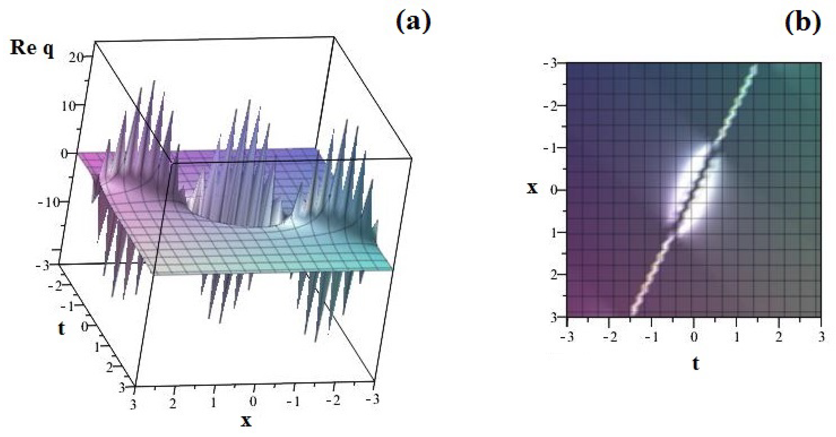
13). All the KMN solutions we got are superpositions between a hyperbolic, periodic or rational amplitude and an oscillating background. Our investigation showed that it is possible to recover all the already known types of solutions, describing bright, dark or singular solitons, periodic or rational oscilations. Behind the traditional solutions, we succeeded to point out, once more, the richness of the model, finding more complex solutions than those already mentioned in literature. For example, the dark soliton expressed by (
46) is more complex as similar solutions pointed out in other papers. Grace of the way we effectively used the solving method, we succeeded to generate quite new solutions, of multi-Peregrine breather type illustrated in the
Figure 1 and
Figure 2 or of multi-solitons as in the
Figure 3.
A more general conclusion, based on the results reported here, but also on those previously reported by other authors, is that the KMN solutions depends on the solving methods, each methods leading to solutions expressed through a given number of parameters. As larger this number is, more complex and sophisticated solutions can be generated.
(2) Beyond these results, a more general objective was to investigate how the KMN solutions depend on the choice of the solving method and of the auxiliary equation. In this is way, in
Section 5 of the paper, the solving method was considered twice, for the two auxiliary equations. In the second case, with a second order auxiliary equation, more complex solutions for KMN were figured out This is because the KMN solutions can depend in this case both on
and on its derivative
. This second dependency is not at all captured by many other solving methods; the
-method and its other versions consider this dependency but only in terms of the ratio,
. The general approach is the big advantage offered by the functional expansion. Another important advantage of the method is related to the type of solutions generated. As these solutions are expressed as expansions of the type (
5) or (
38), they inherit somehow the type of solutions considered for the auxiliary equation. Although, the functional expansion method could generate changes, when
from (
38) are not fractions of polynomials.
(3) A natural problem raised by the previous remark is how could we establish if two solutions belong to the same class? As it was pointed in [
35], it is a quite often situation in various papers to list solutions that, despite the claim of being new ones, are not. This question deserves an extensive study and may lead to two different answers: (i) in the case of the equations generated through a variational principle, the classification of the solutions could be given by the levels of the attached energy; (ii) when non-variational equations are considered, the solutions could be investigated using the Lie symmetry method [
36]. They can be split in classes following the corresponding symmetry operators. A study of this issue for the KMN equation will be presented in a forthcoming paper.


