Planning of Distributed Energy Storage Systems in μGrids Accounting for Voltage Dips


1
Department of Electrical Engineering and Information Technology, University of Naples Federico II, I-80125 Naples, Italy
2
Department of Electrical Engineering and Information “Maurizio Scarano”, University of Cassino and Southern Lazio, I-03043 Cassino, Italy
*
Author to whom correspondence should be addressed.
Energies 2020, 13(2), 401; https://doi.org/10.3390/en13020401
Submission received: 3 December 2019
/
Revised: 8 January 2020
/
Accepted: 10 January 2020
/
Published: 14 January 2020
(This article belongs to the Special Issue Distributed Energy Storage Devices in Smart Grids)
Abstract
:This paper deals with the optimal planning of the electrical energy storage systems in the microgrids aimed at cost minimization. The optimization accounts for the compensation of the voltage dips performed by the energy storage systems. A multi-step procedure, at the first step, identifies a set of candidate buses where the installation of a storage device produces the maximum benefit in terms of dip compensation; then, the life cycle costs in correspondence of different alternatives in terms of size and location of the storage systems are evaluated by considering an optimized use of the energy storage systems. The simulations on a medium voltage microgrid allowed validating the effectiveness of the proposed procedure.
1. Introduction
The role of the systems for storing the electrical energy is gaining more and more importance in the frame of modern power systems. This is thanks to the electrical energy storage systems’ (EESSs) ability to provide a number of benefits across multiple levels [1,2,3]. Focusing on the distribution level of electrical energy systems, the EESSs’ benefits are mainly related to the compensation action of the intermittent effects of renewable power sources and to the support to the operation of the network by providing services aimed at regulating voltage levels, at reducing losses, and deferring the investment on the distribution system [4,5,6]. End-users can also benefit from EESSs through reduction of the cost for the energy purchased as well as for the improvement of power quality (PQ) and reliability [7].
The convenience of the installation of the EESSs is still a critical issue and is strictly related to the number of benefits that can be achieved contemporaneously from their installation [8]. In the case of the microgrids (µGs), cost reduction and PQ improvement are matters of particular interest for both grid operators and end-users.
Cost reduction refers to the ability of the µG owner to increase the share of power produced from renewables inside the µG thus reducing the cost sustained for the imported power, as well as to increase the system efficiency and reduce the network losses. PQ improvement refers to possibility of reducing the level of the PQ disturbances at least up to the ranges admissible for the loads fed by the µG. The typical characteristics of a µG make the objective of the PQ improvement more difficult to attain than in the traditional distribution systems. The network structure, the lengths of the lines, the installed powers and the levels of short circuit power jointly contribute to limiting the PQ robustness of a µG, defined as its intrinsic capacity to maintain assigned disturbance levels when the external conditions change [9,10]. The improvement of the performance of a μG in terms of voltage dips, one of the most critical PQ disturbances, represents an attractive challenge for different reasons. First of all, the voltage dips are the disturbances with serious consequences on processes and activities that could evolve in higher sustained costs. Secondly, these costs are important not only for the industrial users, for which are certainly the most critical [11], but also for commercial and service activities. Loss of production, damages to equipment, halt of processes and data losses are some of the effects of voltage dips, which unavoidably evolve into significant financial losses [12]. Further, the detrimental effects of voltage dips can regard also residential customers, which can suffer for uncomfortable supply service. Also, in the frame of smart grids, most of the new smart technologies are based on electronic devices and control systems, which are particularly sensitive. Finally, it is worth emphasizing that the importance of the improvement of the voltage dip performance is also proved by the fact that most of the regulations on the quality of voltage by the national authorities in Europe started with actions on voltage dips, even if only with wide measurement campaigns like in Italy [13].
In this context, where assuring high voltage dips performance is a primary issue, a possible solution could be given by installing a number of EESSs in the μG, able to fast respond to the occurrence of voltage dips. Clearly, the installation of EESSs is not without drawbacks, particularly those related to the cost of this technology. Thus, EESSs need to be optimally sized by maximizing their benefits while minimizing costs and need to be installed in those nodes considered strategical for the maximization of their value in terms of dip compensation.
In the relevant literature, great effort has been paid to the optimal planning of EESSs in µGs with the objective of the cost reduction. Optimal planning of EESSs in the distribution grids is proposed in [6], based on the minimization of the investment and operation costs. In [14], a planning procedure is proposed, which takes into account the minimization of the cost of energy imported from the external grid while considering voltage support and minimization of network losses. The problem of the optimal siting and sizing of EESSs in μGs is faced in [15] through the minimization of both installation and operation costs, as well as power losses. Minimization of investment and operation costs in distribution networks is considered in the planning tool proposed in [16], which accounts for constraints on bus voltages. Costs of both power losses and EESS’ operation are included in the analytical planning tool presented in [17]. In [18], the optimal allocation of EESSs in distribution networks is performed on the basis of a tradeoff among investment and operation costs, technical constraints and network losses. A planning tool is proposed in [19] aimed at the minimization of installation and operation costs while accounting for the network technical constraints in the presence of uncertainties. The mitigation of voltage dips thanks to the installation of the storage devices is analyzed in [20], where a cost-benefit analysis is proposed. To the best of our knowledge, approaches that include the benefits related to voltage dip compensation within the EESS planning has never been proposed in the current technical literature.
In this paper, a minimum cost strategy for the planning of EESSs in a µG is proposed where the cost is avoided thanks to the voltage dip compensation being taken into account. At this aim, the optimal siting and sizing of EESSs in the µG is formulated in terms of a multi-period, non-linear, constrained optimization problem. A multi-step approach is proposed based on the identification of a limited set of candidate buses among the most exposed to the voltage dips. An optimization tool is used to identify the total cost related to the possible design alternatives (size and location of EESSs). The selection of the candidate buses allows optimizing EESSs’ installation while reducing computational complexity. The reduced computational burden allows analyzing all the possible design alternatives and choosing the optimal solution as the one corresponding to the maximum benefit. Compared to the existing technical literature, the main contribution of this paper in terms of novelty refers to the inclusion of the voltage dips’ cost in the planning of EESSs in µGs.
The paper is organized as follows. The problem formulation of the proposed planning method is reported in Section 2. In Section 3, the method used to identify the set of candidate buses is described. Section 4 reports the optimization tool used to derive the total cost of the planning solutions. Some results related to the application of the proposed method to a case study based on an MV test system are summarized and discussed in Section 5. Our conclusions are drawn in Section 5 together with some comments on future research work.
2. Problem Formulation
The planning problem refers to a three-phase, MV, balanced, µG including residential, industrial and commercial loads. The µG is connected to an upstream grid through the Point of Common Coupling (PCC). The distributed resources including Distributed Generation (DG) units and EESSs are connected to the µG through power converters, and are supposed to be owned by the μG operator.
The contribution of both the DG units and EESSs is the provision of active power to supply part of the loads and, reactive power to support the µG operation. The active power profile of the EESSs (that is, their charging/discharging profile), and the reactive power of both DG units and EESSs are determined on the basis of a minimum cost strategy. More specifically, the strategy is aimed at minimizing the cost sustained by the µG operator for the energy imported from the upstream grid. The size and location of the DG units are assigned whereas, the size and location of the EESSs are identified according to the proposed planning problem based on the minimization, a total cost function. The total cost function includes the installation cost of the EESSs, the operation cost of the μG, and the benefit derived from the voltage dip compensation over the whole planning period.
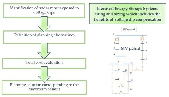
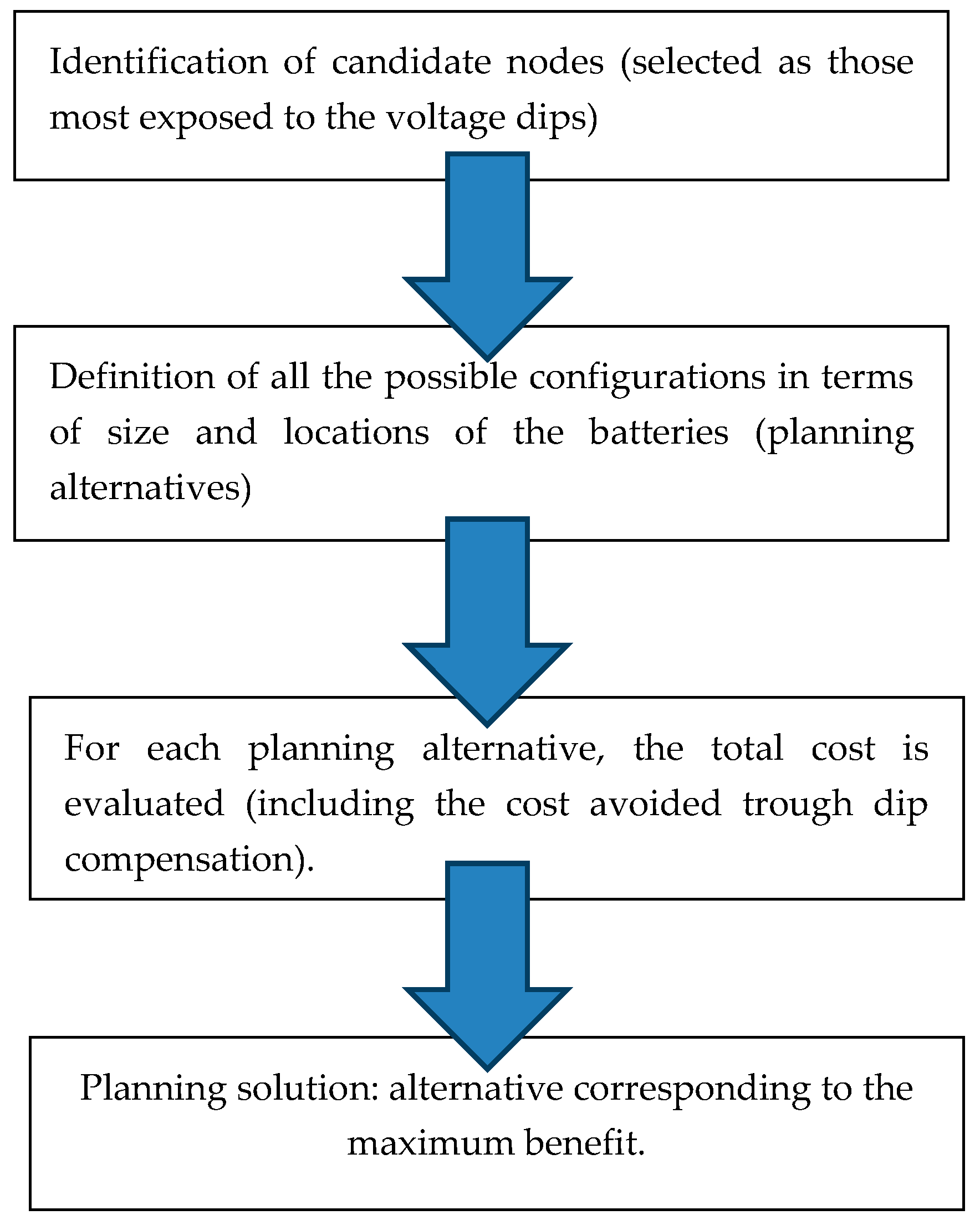
The planning problem is developed in four steps, as shown in the flow chart in Figure 1. The first step refers to the selection of the candidate nodes, chosen as those resulting among the most vulnerable in terms of exposure to the voltage dips. For this reason, these nodes correspond to the sites of the installation of the EES units with the preferred performance in terms of dip compensation. The procedure for the selection is presented in Section 4.
The second step refers to the identification of all the possible configurations in terms of size and location for the EESS installation (limiting the installation only to the set of nodes derived from the Step 1). For each of the possible configurations (planning alternatives), the total cost sustained by the µG owner is evaluated according to the procedure detailed in the Section 5 (third step).
Finally, in the fourth step, the best planning alternative is selected as that corresponding to the maximum benefit (BF) derived by the installation of the EESSs. This BF can be evaluated for each alternative by comparing the total cost sustained by the µG’s owner in absence of the EESSs () and that resulting when the EESSs are installed ():
where is the number of the design alternatives. The total cost evaluated when the EESSs are installed includes the reduction of the cost item related to the voltage dips and of that related to the grid operation thanks to the price arbitrage.
3. Identification of the Set of Buses Most Exposed to the Voltage Dips
A fault in a node can cause a voltage dip in one or more nodes of the electrical network in function of several parameters that determine the electrical power system response to a short circuit. These parameters are linked to the structural characteristics of the network and to the features of the installed components. Examples of such “hardware characteristics” of the electrical system are the network configuration, the installed generator powers, and the size, length and type of the lines.
The numbers of the voltage dips or their frequency in a time horizon, usually one year, is instead linked to the frequency of the causes, the short circuits, which originated them.
The choice of the candidate nodes where the μG operator can place a compensating unit of the voltage dips has been made according to the hardware characteristics of the network that constitutes the μG. In particular, the set of candidate nodes are those nodes that mostly experience the voltage dips whose residual voltage is below a critical value, , regardless the frequency of the faults which originated these voltage dips.
This choice allows ascertaining the sensitiveness of the nodes directly to the effects of the short circuits in any node of the network in terms of voltage dips linked to the characteristics of the network and of the installed components. Consequently, for any possible configuration of the network (radial, meshed, ring) the set of the candidate nodes is different for the same .
Inside a μG, the figure represents the limit value of vulnerability of the loads supplied by the system, that is the minimum value below which the equipment experiences a trip, the most critical effect of a voltage dip.
Theoretically, the value of should vary in function of the specific load fed at every node of the μG. However, a more realistic scenario in a planning stage allows accounting for the vulnerability limits of classes of equipment, as indicated by the International Standards IEC [21]. In the case of equipment supplied by the μG are of Class II or Class III, corresponds to the limit value of 70% or 40% of the declared voltage, respectively, for the voltage dips lasting up to 200 ms.
Summarizing, for every possible configuration of the μG network, the set of candidate busses for the installation of a compensating units is the set of busses which experience the largest number of voltage dips whose residual voltage is below , regardless the frequency of the faults which caused these voltage dips.
The Fault Position Method (FPM) is the most effective tool for the selection of the candidate bus set in the given assumptions.
In fact, for a system with nodes the FPM allows obtaining the (x) matrix of the during fault voltages in any node for short circuit in every node, , by means of the following equation for a three-phase fault in every node of the system:
where is the nodal short circuit impedance matrix, is the pre-fault voltage matrix and is the matrix formed by the inverse of the diagonal elements of the short circuit impedance matrix. If the pre-fault voltages are assumed to be 1 p.u., relation (2) can be written as:
where is a matrix full of ones and such that dimension is equal to the dimension of .
Any element of with magnitude less than 0.9 p.u. represents a voltage dip in the node caused by a three-phase short circuit in the node . For different types of short circuits, similar equations can be drawn [22].
For every network configuration of the μG with nodes, starting from the matrix obtained by the FPM, the set of candidate busses is chosen as constituted by the nodes such that:
As mentioned above, the value of in the equation (4) is chosen from the Standard (e.g., [23]).
4. Total Cost Evaluation
For each alternative, the total costs, , related to the inclusion of the EESSs in the µG is given by the sum of the cost of installation, , and replacement, , of the EESSs, the operation costs of the µG, , and the cost due to voltage dips.
All the cost items refer to the whole planning period and are detailed in the following sub-sections. In (5), maintenance cost can be also added as a percentage of the installation cost. For ease of notation, in the following equations, the reference to alternative is omitted.
4.1. Installation Cost
The installation cost includes both the cost of the battery and the cost of the power converter interfacing the storage device to the grid. The cost of the battery depends on the energy capacity, whereas the cost of the power converter is related to the rated power. In case of EESSs, the rated energy and power are linked through the nominal C-rate. Then, a unitary installation cost can be provided once the nominal C-rate has been specified. In this case, the installation cost of the EESSs is given by the product of the capacity unitary installation cost, , and the battery size. Obviously, the former depends on the considered battery technology and the latter refers to the specific design alternative. The installation cost is then given by:
where is the number of installed EESSs and is the size of the ith EESS.
4.2. Replacement Cost
Based on the expected battery lifetime, which is given in terms of number of charging/discharging cycles—and that depends on the battery’s stress factors, the replacement of the device could be necessary during the considered planning period. The replacement cost is given by:
where is the unitary cost for the battery replacement, and indicates the number of times the ith battery needs to be replaced. To evaluate the battery’s lifetime duration must be evaluated and compared to the planning period. The battery’s lifetime, in years, () can be evaluated based on the lifecycle (i.e., life expressed in terms of number of charging/discharging cycles), , and on the number of cycles per day, :
represents the total number of cycles the battery can be used before the replacement; it strictly depends on the battery technology and on the way stress factors act [24,25]. Its value is provided by the battery manufacturer, and it is related to specified operation conditions, such as ambient temperature and depth of discharge (DoD). The value of depends on the way the battery is operated, which depends on the operation strategy.
4.3. Operation Cost
The operation cost of the µG refers to the cost of the energy imported from the upstream grid. It is supposed that the µG is not able to sell energy to the upstream grid. The cost of the energy imported implies the evaluation of the overall costs
- -
- sustained by the µG’s owner to (i) supply the loads, (ii) charge the EESSs, (iii) compensate for the power losses;
- -
- avoided thanks to the EESS discharged energy.
The planning time horizon includes years, each represented by typical days. Forecasted daily profiles of the power requested by the loads, of the power delivered by the distributed generation, and those of the energy price are known for each typical day of the first year. These profiles are known with reference to all the time intervals—of duration —in which each day is divided. The corresponding profiles for the subsequent years are evaluated based on a specified yearly growth. The operation cost for the whole planning period is then provided by the net present value of the sum of the costs sustained at each typical day:
where is the discount rate, is the number of days represented by the dth typical day in the year , and are the power imported from the upstream network and the energy price, respectively, at the kth time interval of the dth typical day of the year .
In order to evaluate the power imported from the upstream grid, , a minimum cost strategy is formulated for the µG, on the basis of a two-stage procedure which allows decoupling the hourly optimization algorithm so reducing the computational burden.
In the first stage, the hourly active power of the EESSs is evaluated. According to the cost minimization approach, the value of the power of each EESS is derived by charging the battery during low-price hours and discharging it during the high price hours, while constraints are imposed on the rated power and energy capacity of the EESSs.
In the second stage an OPF is solved, at each time interval, with respect to the known variables (i.e., specified values of loads’ active and reactive powers and active powers of DG units and EESSs) and unknown variables (i.e., active and reactive power at the PCC, reactive powers of both DG units and EESSs.) Coherently with the cost minimization strategy, the OPF minimizes the power imported at the PCC while satisfying the constraints on both the µG and the interfacing converters.
a. 1th Stage: EESS Profile Optimization
The power that can be charged or discharged by the EESSs at each time interval depends on the stored energy available in the battery, on the rated power and on the price of energy corresponding to that interval. A this aim, two sets of time intervals are identified in a day: the first set is related to the highest price—where the EESSs can be discharged to reduce the costs of the imported power—, the second set is related to the lowest price—where the EESSs can be charged—. Two different iterative procedures are applied in and (Figure 2).
The iterative procedure that applies to allows obtaining the EESS’s profile during the discharging stage (Figure 2a). The procedure is based on the identification of the time intervals included in and on the identification of the set which includes the time intervals of sorted by decreasing price of energy. Then, at each time interval tk included in , with , the power discharged by the battery is identified as the minimum between the EESS rated power () and the power corresponding to the battery SoC ():
With reference to the first interval in which the battery can be discharged, , it is assumed that the battery is fully charged, thus
where is the rated energy capacity of the battery, and is the admissible DoD. Once the battery power is known through (10), the power corresponding to the SoC is updated:
where is the discharging efficiency of the EESS. The procedure ends when all of the time intervals in are explored (i.e., ) or . Outputs of the procedure are the EESSs’ power profiles during the discharging stage (i.e., ) and the total energy which can be discharged by the battery:
The iterative procedure, which applies in allows obtaining the EESS’s profile during the charging stage (Figure 2b). The procedure is based on the identification of the time intervals included in and on the identification of the set which includes the time intervals of sorted by increasing price of energy. Then, at each time interval th included in , with , the discharged power of the battery is identified as the minimum between the EESS rated power () and the power corresponding to the battery SoC ():
With reference to the first interval in which the battery can be charged, , it is assumed that the battery is empty, thus
where is given by (13). Once the battery power is known through (10), the power corresponding to the SoC is updated:
Where is the charging efficiency of the EESS. The procedure ends when all of the time intervals in are explored (i.e., ) or . Outputs of the procedure are the EESS’s power profile during the charging stage (i.e., ) and the total energy, which can be charged by the battery:
In order to make the strategy feasible, it is required that during each day, the energy charged and discharged must be the same:
In the case that (18) is not satisfied, the procedure for the discharging stage (Figure 2) must be repeated by replacing .
b. 2nd Stage: Optimal Power Flow
The Optimal Power Flow (OPF) in its general form is formulated as:
where the minimization of the objective function is subject to equality and inequality constraints, and applied to the vector of the optimization variables. Inputs of the OPF are the forecasted values of the power load demand, the DG power production, the energy price and the EESS power. Outputs are the reactive power of the DG units and of the EESSs, and the active and reactive power at the PCC. All these quantities are required to be known at all the time intervals of each typical day of year . In order to minimize the operation costs defined in (9), the objective function is:
The constraints to be satisfied in the OPF include the classical power flow equations:
where is the number of network buses and, with reference to the time interval of the day in the year is the difference between the phase angles at nodes and , and are the active and reactive powers at bus , is the bus voltage amplitude, and are the -terms of the matrices of the conductance and susceptance, respectively. Constraints (25) and (26) refer to slack bus (), that is the PCC.
The active and reactive powers in (19) and (20) include the powers absorbed by the loads, the power charged/discharged by the EESSs and the power produced by the DG units.
The active and reactive power exchanged at the PCC must comply with the transformer rate, , that is:
The same applies to the power flowing through the converters interfacing the EESSs and the DG units, which cannot exceed the converter rated power, :
where has been previously derived in Step 1, is the EESS reactive power, and and are the DG active and reactive powers, and are the sets of buses, where the EESSs DG units are connected, respectively.
Further constrains refer to the limits imposed to the bus voltage and line current magnitudes:
being and the minimum and maximum voltage magnitude values, the current flowing through the lth line of the set of network lines, which cannot exceed the maximum value, (i.e., line ampacity).
In this case, the 2nd stage does not converge due to constraint violation, it will be iteratively applied by reducing the EESS contribution (i.e., by reducing ), till convergence is reached.
4.4. Cost of Voltage Dips
The cost of the voltage dips is strictly connected to the economic value the effects of the voltage dips have on the equipment’s and the operating processes or the activities. The most critical effect of the voltage dips is the trip of the device that is subject to the dip. The economic value of this detrimental effect represents, in turn, the cost of the voltage dip, and depends on the function of the device into the process or activity, the type of the process or activity, the linkage of the process in case stopped with other processes of the same production line, in case of industrial manufacturing loads, or with other operative functions, in case of loads different from manufacturing industries.
Generally, the cost of the voltage dips is the sum of three main components: direct, indirect and hidden costs [23]. The direct costs relate to the interruptions of the specific device or equipment. They include, for example, lost work, lost production, damaged equipment; the indirect costs include the investment costs sustained by the end user to prevent or to solve the damages due the interruptions caused by voltage dips. Finally, the hidden costs account for any second level effects that reflect on the performance of the business, such as retaining customers, satisfying customers, and protecting the company’s reputation. The hidden costs in some studies are included inside the indirect costs [26].
The cost of the voltage dips can be estimated by means of direct methods or indirect methods.
The direct methods are analytical methods that require at least the availability of the voltage dips measured at the load site, the deep knowledge of several characteristics of the devices or equipment (dip susceptibility curve, operating mode, functional linkage of each device with other devices of the same equipment, and of the same process, structure and topology of the electric lines feeding each device and equipment), and the detection of the areas of the process exposed to the stoppage. They are usually conducted as after-the-fact-case studies of the events of voltage dips occurred at a specific site [26,27,28]. A direct method can also use the voltage dips expected at the site feeding the sensitive loads obtained by means of the simulation of the electric system in short circuit conditions. The two main methods available and widely used are the fault position method (FPM) and the critical distance method (CDM). The most adequate method to use depends on several parameters, as reported in the comparative study of [8]. Whichever of these methods obviously requires the knowledge of the electrical system feeds the load sites.
The indirect methods estimate the cost of a disturbance without passing through the analytical quantification of the effects of that disturbance on specific devices or equipment’s. They can use macroeconomic analysis [11] or surveys of the customers asked to directly estimate their suffered costs due to the supply disturbances or to provide qualitative economic figures of the electric supply linked to that disturbance. In the case of the supply interruptions, for example, the National economic regulation of continuity in Italy started with an extensive survey aimed to estimate two indices: the willingness to pay (WTP) and the willingness to accept (WTA) [29]. WTP measures the additional price of the electric service the users would pay for avoiding the interruptions; WTA instead measures the amount of money they would accept for having to experience the outage. These indices allowed fixing the incentive rate for the penalties and the rewards in the first regulatory scheme of the National Authority of electricity ARERA, formerly AEEG [30].
The existence of the economic regulation of a disturbance could solve the problem of establishing the costs for the loads, especially in the planning activities with long-term horizons, as in the case of this study. In such cases, in fact, the specific details of the loads are not obtainable and would not be reliable to assign them.
Unfortunately, no economic regulation of the voltage dips is still active [31]. However, some preliminary studies [32,33] offer valuable figures resulting from measurements, survey and simulations, which can guide in deriving the economic value to assign to the voltage dips.
In this paper, we referred to [32] where the authors analyzed the economic and technical data collected for a number of medium-voltage (MV) industrial users that participated in the cost assessment project and the monitoring campaign. In particular, the authors used an indirect method based on a monitoring-and-survey approach to estimate the direct costs faced by a large variety of industrial customers. As detailed in the paper, the costs were presented both as annual value per kW and as event value for kW, with the latter independent from frequency. In this paper, we used the event value per kW of the installed power of the load.
For the evaluation of the total costs of the voltage dips over a long-time horizon, the frequency of occurrence of the voltage dips must be evaluated. The annual frequency can be estimated in average from data measured on real systems. In this paper, we referred to the measured data on the MV Italian National Grid (with reference to year 2016) at the MV busbars of the HV/MV substations (Table 1) [34].
Finally, the cost related to voltage dips over the planning period, , can be evaluated as:
where is the number of busses sensitive to the voltage dips, is the planning time horizon (years), is the discount rate and, with reference to the voltage dip belonging to the residual voltage class, rv, is the cost suffered by the customer due to the single event of voltage dip at the year , is the number of the voltage dip events at year , and is the set of residual voltage classes which the voltage dip event refers to (i.e., first column of Table 1). is the power value to be considered for the dip cost identification, with reference to the user connected to the ith bus of the µG at year . In this paper, we referred to the load nominal value.
We assumed that the EEC units compensate only to voltage dips at the node where the EES is installed. This assumption is very cautious, since the beneficial effects of the compensating action can be wider, involving also further nodes electrically close to the installation node of the EES. With structures of the network other from radial, the detection of the area, in which the voltage dips are compensated by the EES installed in one node, requires the simulation of the system in short circuit conditions with EES acting as voltage dip compensating unit. A FPM, applied in the presence of the EES, giving as result the propagation of the voltage dips for short circuits in every node of the system, could allow obtaining this result.
5. Numerical Applications
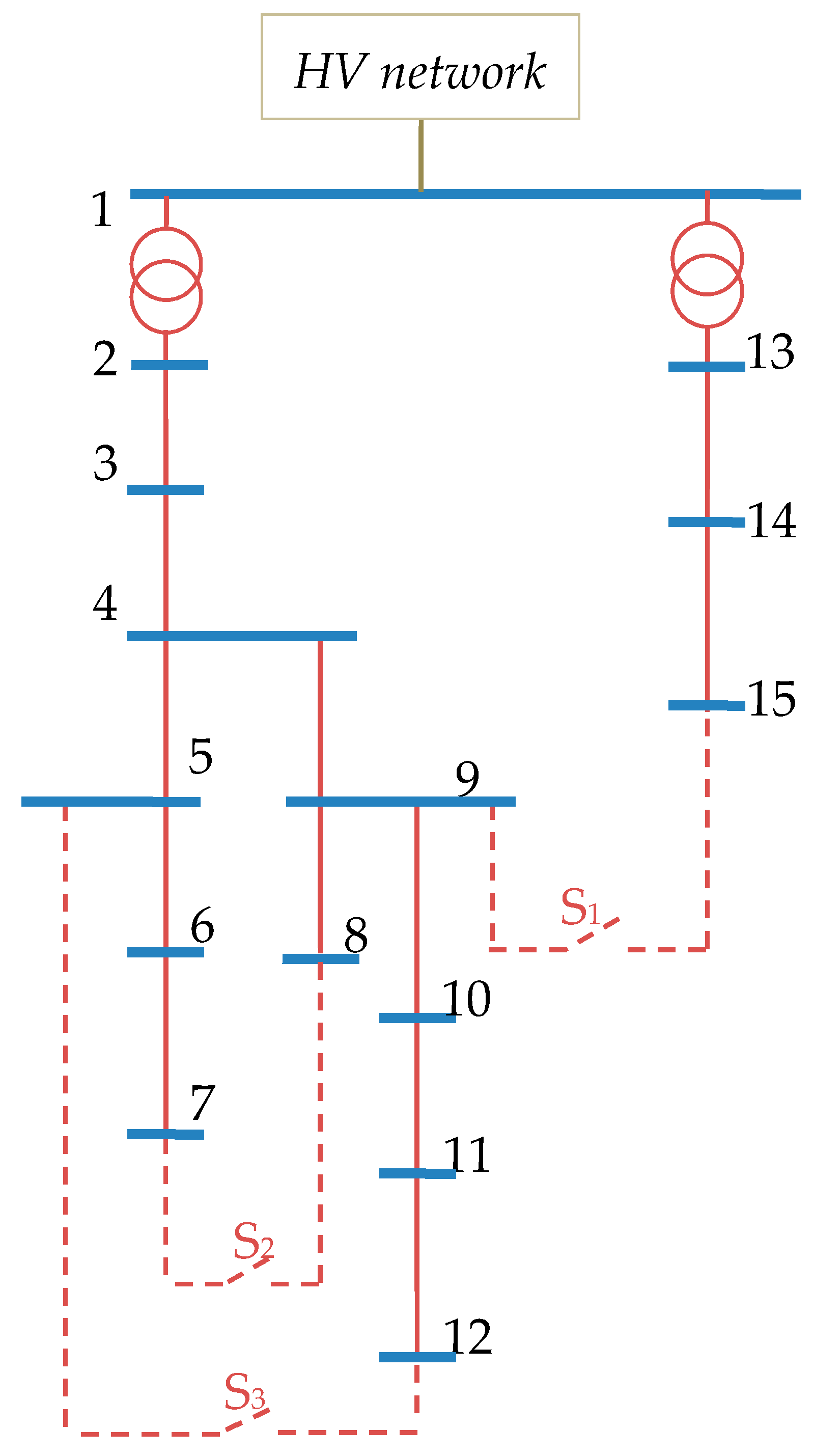
The planning procedure has been applied to an MV µG, which refers to the MV Cigrè benchmark system [35]. The system under study is a 12.47 kV, three-phase, balanced, distribution network (Figure 3). This network is constituted by 15 buses and it is connected to an upstream HV network by means of two 115/12.47 kV transformers of 25 and 20 MVA, which connect the PCC (bus #1) to two feeders: the first feeder is connected at the secondary side of the 25 MVA transformer (bus #2); the second feeder is connected at the secondary side of the 20 MVA transformer (bus #13). The network includes three switches: S1 (between buses #9 and #15), S2 (between buses #7 and #8) and S3 (between buses #5 and #12).
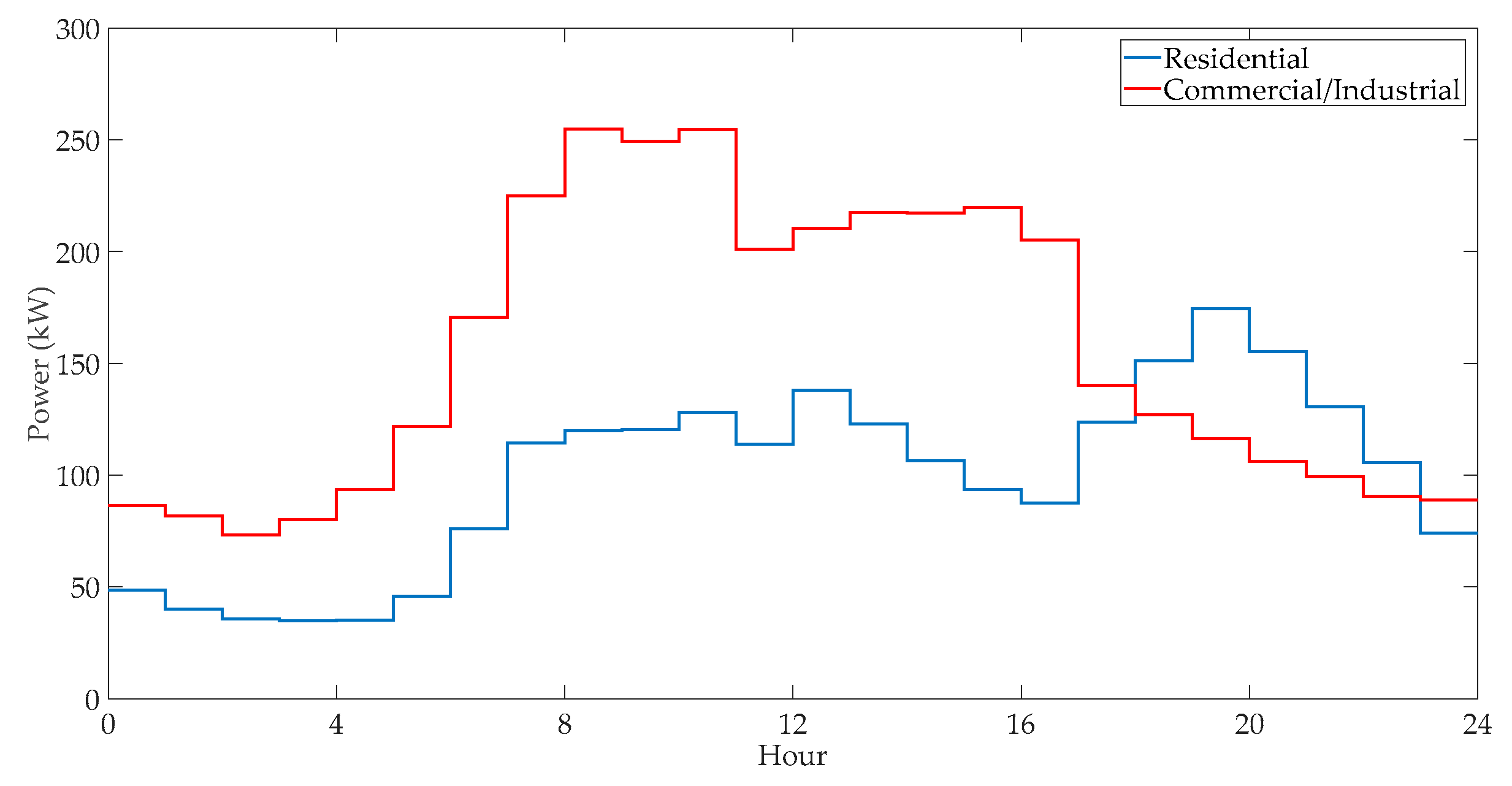
The loads connected to the network are grouped in residential and commercial/industrial and are listed in Table 2. The loads are assumed to have a yearly growth of 1%. The per unit power profiles assumed for residential and industrial/commercial customers are reported in Figure 4. Two PV units are connected to the buses #9 and #15 with rated powers of 5 MW and 2 MW, respectively. Figure 5 shows the per unit power profile of the PV generation at bus #9.
The assumed energy pricing tariff refers to the hourly values of the Italian market price. With reference to the first year, the price values refer to a day of November 2019 [36] (Figure 6). A yearly growth of 1% has also been assumed for the energy prices. Regarding the cost, which the customers have to sustain due to the single voltage dip event, the value 2.9 €/kW [32] has been assumed with a yearly growth of 1% for the industrial/commercial loads; for the residential loads, instead, the value of zero was assumed. The number of events is evaluated according to the data reported in Table 1. Particularly, the events related to the threshold voltage dip value, Vcr, of 70% has been assumed.
Regarding the EESSs to install, nickel manganese cobalt Li-ion battery technology has been considered suitable for this application. The data of the various EESS’ features are reported in Table 3 [37], which refer to values expected for 2020. Regarding the battery replacement cost, the value of the cost expected for the 2025 has been considered. Note that the costs in Table 3 have been converted in Euro (conversion rate of November 2019) before applying them in the proposed procedure.
The planning design alternatives refer to the installation of two EESSs whose size must be selected among the rated power values 0, 5, 10 and 15 MW with a discharging nominal time of five hours.
In order to show the ability of the method to satisfy the technical constraints imposed on the EESSs and on the µG, Figure 7 and Figure 8 report the daily profiles of the active power of an EESS and of the voltage values at the buses where an EESS and a PV unit are connected. The figures refer to the first year of the planning period of the case study 1 and detail the profiles of the EESS connected at the bus #6 and of the PV unit connected at the bus #15.
During the µG operation, the breakers can be operated open or closed depending on the operator decisions aimed at avoiding undesired conditions or based on economic strategies. The states of the breakers strongly affect the values that line currents and bus voltages can assume. In order to consider the influence of the states of the breakers in terms of exposure of the buses to the voltage dips, the proposed planning procedure has been applied with reference to the following case studies:
- -
- Case 1: S1, S2, S3: open
- -
- Case 2: S1, S2, and S3: closed
- -
- Case 3: S1: closed, S2, S3: open
- -
- Case 4: S1, S3: open, S2: closed
- -
- Case 5: S1, S2: open, S3: closed
- -
- Case 6: Case 1 (0.45), Case 2 (0.10), Case 3 (0.15), Case 4 (0.15), Case 5 (0.15)
Case 6 refers to the probability of occurrence of different network configurations (the probability of occurrence of each configuration is indicated within the brackets).
The application of the procedure of Section 3 for the identification of candidate buses based on voltage dip sensitiveness leads to the candidate buses reported in Table 4 that correspond to the threshold voltage dip value of 70%. The results of the planning procedure corresponding to each case study are reported in Table 5. In the table, the BF of each planning solution is reported together with the reduction of the cost of voltage dips obtained thanks to the installation of the EESSs. For comparative purposes, the planning results are reported for both the cases in which the reduction of voltage dip cost is taken into account and those in which this cost reduction is neglected. Negative values of BF are obtained in the cases where installation of EESSs is not convenient.
The results reported in Table 5 show that the convenience of installing EESSs in the μG basically depends on the cost reduction obtained thanks to the price arbitrage. In fact, in the cases where the price arbitrage does not allow installing EESSs (cases 2 and 3), the added benefits derived from the voltage dip compensation is not sufficient to justify the adoption of the storage devices. This is probably due to the fact that, being the candidate buses mainly characterized by residential loads, the benefit derived by dip compensation in terms of cost reduction is not significant (we remind that the cost of voltage dip for the residential load was neglected). Moreover, in the cases where it is convenient to install the EESSs (cases 1, 4, 5, and 6) the beneficial effect of dip compensation clearly appears only when they are used in buses with large industrial loads. In fact, in cases 4 and 5, the installation of the EESS n. 2 in bus #6 instead of bus #4 and in bus #6 instead of bus #5, respectively, allows obtaining higher benefits.
In order to better prove the effect of the dip compensation on the total cost reduction, in Table 6, the percentage values of the benefit related to the voltage dip cost reduction are reported, with reference to the cases in which the planning procedure provides a solution. It is interesting to note that the percentage benefit due to the voltage dip cost reduction falls within the range [33,34,35] % in cases 1, 4, and 5. In case 6, the percentage value is lower (about 11%). This is mainly due to the fact that in case 6, the solution associated to the largest total benefit corresponds to allocation buses (buses #8 and #10) with voltage dip costs lower than those corresponding to the nodes selected in cases 1, 4, and 5.
In Table 6, the percentage values of the benefit corresponding to the voltage dip reduction compared to the EESS’s installation and replacement costs are also reported. The value of about 6% is obtained in the cases 1, 4 and 5. A lower value (about 2%), instead, is obtained in case 6. This is due to two aspects: the first refers again to the reduced benefit in terms of voltage dip cost reduction (compared to the other cases), the second refers to the increased size of storage, which is allocated in this case study.
Figure 7 clearly shows that the maximum power that is charged/discharged by the EESS is always lower than the rated power. Moreover, the comparison of Figure 6 and Figure 7, reveals that the battery absorbs power during the lowest price hours, and injects power to the grid during the highest price hours. This is coherent with the considered minimum cost strategy. The SoC profile—here not reported for the sake of conciseness—also satisfies the constraints on the rated battery capacity.
Figure 8 shows that the voltage at the critical buses, i.e., the buses where an EESS or a DG are connected, falls within admissible ranges (0.9–1.1) p.u. The increased variation of the voltage in the nodes where an EESS is connected which appears in the figure is due to the charge/discharge of the EESS. In the node where a DG is connected, instead, a smooth profile appears; this is due to the power rating of the generation system lower than that of the EESS and to the presence of the high load power in the buses close to this node.
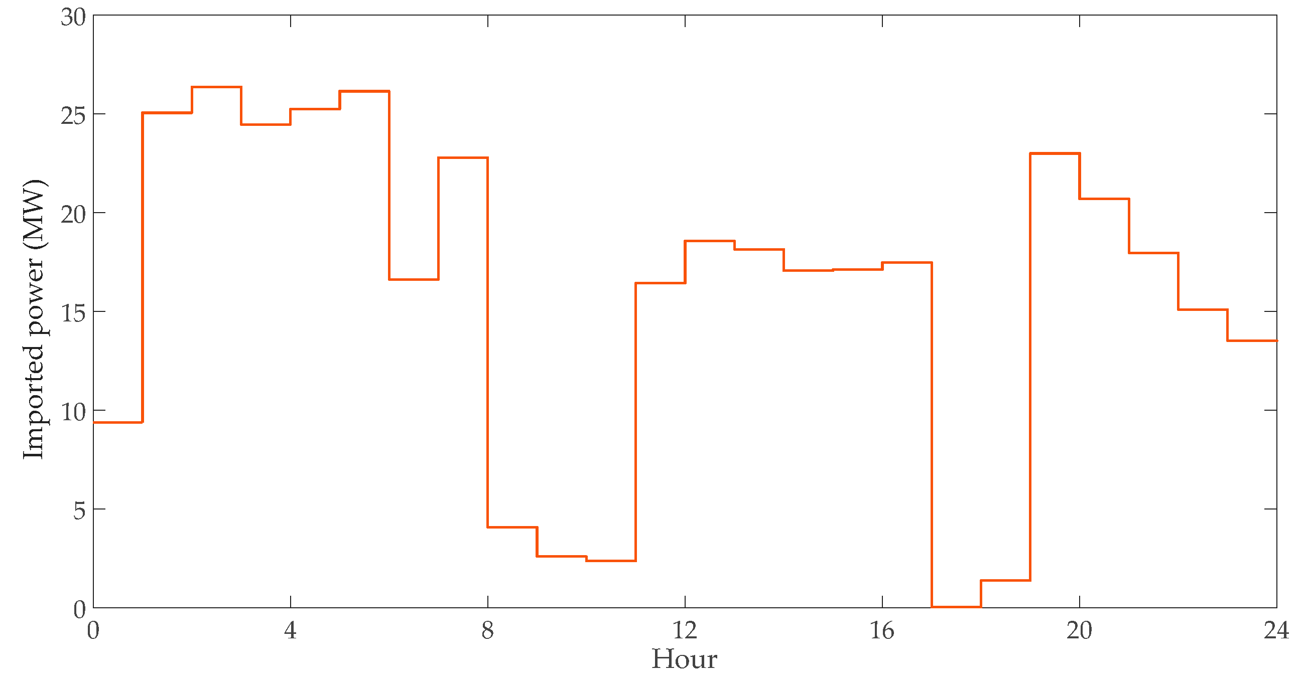
Still referring to the case study 1—first year of the planning period—Figure 9 shows the active power imported at the PCC. Coherently with the minimum cost strategy, thanks to the use of the EESSs, most of the requested power is shifted from the highest price hours to the lowest price hours.
6. Conclusions
In this paper, the planning of the electrical energy storage systems in the microgrids was considered. A cost minimization approach was proposed including the benefits obtained through the voltage dip compensation. Particularly, the cost reduction is obtained by shifting the load from the hours of high energy price to those of low energy prices and by considering the voltage dip cost avoided thanks to the compensation action. The motivation of this study is twofold. The first relies on the importance of power quality aspects in the modern power systems characterized by widespread use of electronic devices and control systems which are highly vulnerable to the voltage dips. The latter refers to the benefits derived from the ability the storage systems have in providing multiple services, which concur to sustain their high installation cost. The proposed method is based on a multi-step planning tool which allows identifying the optimal location and size of the storage systems. The results of the numerical simulations clearly showed that voltage dip compensation allowed obtaining non-negligible economic benefits. Clearly, these benefits strictly depend on the cost assumed for the voltage dip events, which can be specified only through a deep knowledge of the end-users. Future works will be aimed at improving the procedure in order to better identify the areas of the network that achieve a beneficial effect in terms of dip compensation from the installation of EESSs.
Author Contributions
F.M., D.P., P.V. (Pietro Varilone) and P.V. (Paola Verde) conceived and designed the theoretical methodology and the numerical applications; F.M., D.P., P.V. (Pietro Varilone) and P.V. (Paola Verde) performed the numerical applications and analyzed the results; F.M., D.P., P.V. (Pietro Varilone) and P.V. (Paola Verde) wrote and revised the paper. All authors have read and agreed to the published version of the manuscript.
Funding
Financial support by Italian Ministry of University and Research (MIUR) through the Special Grant “Dipartimenti di eccellenza” Lex. N. 232/31.12.2016 (G.U. n. 297/21.12.2016 S.O. n. 57).
Acknowledgments
The authors thank Guido Carpinelli (University of Naples Federico II) for his invaluable and generous contribution in the continuous development of new ideas to deal with increasingly interesting problems of modern power systems. The authors P. Varilone and P. Verde acknowledge the financial support by Italian Ministry of University and Research through the Special Grant “Dipartimenti di eccellenza”.
Conflicts of Interest
The authors declare no conflict of interest.
References
- Ai Wong, L.; Ramachandaramurthy, V.K.; Taylor, P.; Ekanayake, J.B.; Walker, S.L.; Padmanaban, S. Review on the optimal placement, sizing and control of an energy storage system in the distribution network. J. Energy Storage 2019, 21, 489–504. [Google Scholar] [CrossRef]
- Hemmati, R.; Shafie-Khah, M.; Catalão, J.P.S. Three-Level Hybrid Energy Storage Planning Under Uncertainty. IEEE Trans. Ind. Electron. 2019, 66, 2174–2184. [Google Scholar] [CrossRef]
- Zhang, N.; Li, R.; Jiang, Y. Cost-benefits analysis of battery storage system for industry consumers based on different operation modes. In Proceedings of the 2018 IEEE 2nd International Electrical and Energy Conference (CIEEC), Beijing, China, 4–6 November 2018; pp. 527–531. [Google Scholar] [CrossRef]
- Saboori, H.; Hemmati, R.; Sadegh Ghiasi, S.M.; Dehghan, S. Energy storage planning in electric power distribution networks—A state-of-the-art review. Renew. Sustain. Energy Rev. 2017, 79, 1108–1121. [Google Scholar] [CrossRef]
- Carpinelli, G.; Celli, G.; Mocci, S.; Mottola, F.; Pilo, F.; Proto, D. Optimal Integration of Distributed Energy Storage Devices in Smart Grids. IEEE Trans. Smart Grid 2013, 4, 985–995. [Google Scholar] [CrossRef]
- Grover-Silva, E.; Girard, R.; Kariniotakis, G. Optimal sizing and placement of distribution grid connected battery systems through an SOCP optimal power flow algorithm. Appl. Energy 2018, 219, 385–393. [Google Scholar] [CrossRef] [Green Version]
- Carpinelli, G.; Mottola, F.; Proto, D. Probabilistic sizing of battery energy storage when time-of-use pricing is applied. Electr. Power Syst. Res. 2016, 141, 73–83. [Google Scholar] [CrossRef]
- Electricity Energy Storage Technology Options: A White Paper Primer on Applications Costs and Benefits. 2010. Available online: https://www.epri.com/ (accessed on 12 January 2020).
- Carpinelli, G.; Di Perna, C.; Caramia, P.; Varilone, P.; Verde, P. Methods for Assessing the Robustness of Electrical Power Systems Against Voltage Dips. IEEE Trans. Power Deliv. 2009, 24, 43–51. [Google Scholar] [CrossRef]
- Caramia, P.; Varilone, P.; Verde, P.; Vitale, L. Tools for Assessing the Robustness of Electrical System against Voltage Dips in terms of Amplitude, Duration and Frequency. In Proceedings of the International Conference on Renewable Energies and Power Quality (ICREPQ’14), Cordoba, Spain, 8–10 April 2014. [Google Scholar]
- Küfeoğlu, S.; Lehtonen, M. Macroeconomic Assessment of Voltage Sags. Sustainability 2016, 8, 1304. [Google Scholar] [CrossRef] [Green Version]
- Ding, Z.; Zhu, Y.; Chen, C. Economic loss assessment of voltage sags. In Proceedings of the CICED 2010 Proceedings, Nanjing, China, 13–16 September 2010; pp. 1–5. [Google Scholar]
- 6th CEER Benchmarking Report on the Quality of Electricity and Gas Supply; CEER, 2016. Available online: https://www.ceer.eu/1305/ (accessed on 12 January 2020).
- Nick, M.; Cherkaoui, R.; Paolone, M. Optimal siting and sizing of distributed energy storage systems via alternating direction method of multipliers. Int. J. Electr. Power Energy Syst. 2015, 72, 33–39. [Google Scholar] [CrossRef]
- Nojavan, S.; Majidi, M.; Esfetanaj, N.N. An efficient cost-reliability optimization model for optimal siting and sizing of energy storage system in a microgrid in the presence of responsible load management. Energy 2017, 139, 89–97. [Google Scholar] [CrossRef]
- Lin, Z.; Hu, Z.; Zhang, H.; Song, Y. Optimal ESS allocation in distribution network using accelerated generalised Benders decomposition. IET Gener. Transm. Distrib. 2019, 13, 2738–2746. [Google Scholar] [CrossRef]
- Fantauzzi, M.; Lauria, D.; Mottola, F.; Scalfati, A. Sizing energy storage systems in DC networks: A general methodology based upon power losses minimization. Appl. Energy 2017, 187, 862–872. [Google Scholar] [CrossRef]
- Nick, M.; Cherkaoui, R.; Paolone, M. Optimal Allocation of Dispersed Energy Storage Systems in Active Distribution Networks for Energy Balance and Grid Support. IEEE Trans. Power Syst. 2014, 29, 2300–2310. [Google Scholar] [CrossRef]
- Andreotti, A.; Carpinelli, G.; Mottola, F.; Proto, D.; Russo, A. Decision Theory Criteria for the Planning of Distributed Energy Storage Systems in the Presence of Uncertainties. IEEE Access 2018, 6, 62136–62151. [Google Scholar] [CrossRef]
- Celli, G.; Pilo, F.; Pisano, G.; Soma, G.G. Including voltage dips mitigation in cost-benefit analysis of storages. In Proceedings of the 2018 18th International Conference on Harmonics and Quality of Power (ICHQP), Ljubljana, Slovenia, 13–16 May 2018; pp. 1–6. [Google Scholar] [CrossRef]
- IEC 61000-4-11:2004. Testing and Measurement Techniques—Voltage Sags, Short Interruptions and Voltage Variations Immunity Tests. 2004. Available online: https://webstore.iec.ch (accessed on 12 January 2020).
- Carpinelli, G.; Caramia, P.; Di Perna, C.; Varilone, P.; Verde, P. Complete Matrix Formulation of Fault Position Method for Voltage Dip Characterization. IET Gener. Transm. Distrib. 2007, 1, 56–64. [Google Scholar] [CrossRef]
- IEEE Standard 1346. Recommended Practice for Evaluating Electric Power System Compatibility with Electronic Process Equipment; The Institute of Electrical and Electronics Engineers, Inc.: New York, NY, USA, 1998. [Google Scholar]
- Xu, B.; Oudalov, A.; Ulbig, A.; Andersson, G.; Kirschen, D.S. Modeling of Lithium-Ion Battery Degradation for Cell Life Assessment. Trans. Smart Grid 2018, 9, 1131–1140. [Google Scholar] [CrossRef]
- Han, X.; Lu, L.; Zheng, Y.; Feng, X.; Li, Z.; Li, J.; Ouyang, M. A review on the key issues of the lithium ion battery degradation among the whole life cycle. ETransportation 2019, 1, 100005. [Google Scholar] [CrossRef]
- Fumagalli, E.; Lo Schiavo, L.; Delestre, F. Service Quality Regulation in Electricity Distribution and Retail; Springer: Berlin/Heidelberg, Germany, 2007. [Google Scholar]
- Di Fazio, A.R.; Duraccio, V.; Varilone, P.; Verde, P. Voltage sags in the automotive industry: Analysis and solutions. Electr. Power Syst. Res. 2014, 110, 25–30. [Google Scholar] [CrossRef]
- Weldemariam, L.; Cuk, V.; Cobben, J. Cost Estimation of Voltage Dips in Small Industries Based on Equipment Sensitivity Analysis. Smart Grid Renew. Energy 2016, 7, 271–292. [Google Scholar] [CrossRef] [Green Version]
- Bertazzi, A.; Fumagalli, E.; Lo Schiavo, L. The use of customer outage cost surveys in policy decision-making: The Italian experience in regulating quality of electricity supply. In Proceedings of the CIRED 2005—18th International Conference and Exhibition on Electricity Distribution, Turin, Italy, 6–9 June 2005; pp. 1–5. [Google Scholar]
- Delibera n. 155/02, Testo Integrato delle Disposizioni Dell’autorità per L’energia Elettrica e il Gas in Materia di Continuità del Servizio di Distribuzione Dell’energia Elettrica, G.U. Serie Generale n. 201 del 28 Agosto 2002. Available online: https://www.arera.it/it/docs/02/155-02.htm (accessed on 12 January 2020). (In Italian).
- Bollen, M.; Beyer, Y.; Styvactakis, E.; Trhulj, J.; Vailati, R.; Friedl, W. A European Benchmarking of voltage quality regulation. In Proceedings of the 2012 IEEE 15th International Conference on Harmonics and Quality of Power, Hong Kong, China, 17–20 June 2012; pp. 45–52. [Google Scholar]
- Delfanti, M.; Fumagalli, E.; Garrone, P.; Grilli, L.; Lo Schiavo, L. Toward Voltage-Quality Regulation in Italy. IEEE Trans. Power Deliv. 2010, 25, 1124–1132. [Google Scholar] [CrossRef]
- Weldemariam, L.E.; Cuk, V.; Cobben, J.F.G. A proposal on voltage dip regulation for the Dutch MV distribution networks. Int. Trans Electr. Energy Syst. 2019, 29, e2734. [Google Scholar] [CrossRef] [Green Version]
- Relazione Annuale Sullo Stato dei Servizi e Sull’ Attività Svolta. AEEGSI Annual Report AEEGSI. 2018. Available online: www.autorita.energia.it (accessed on 12 January 2020). (In Italian).
- Benchmark Systems for Network Integration of Renewable and Distributed Energy Resources, Cigré Task Force C6.04, Cigré Brochure 575. 2014. Available online: https://e-cigre.org/ (accessed on 12 January 2020).
- Gestore Mercati Energetici. Esiti Mercato Elettrico, November 2019. Available online: https://www.mercatoelettrico.org/it/ (accessed on 12 January 2020).
- IRENA. Electricity Storage and Renewables: Costs and Markets to 2030, International Renewable Energy Agency, Abu Dhabi. 2017. Available online: http://www.irena.org/publications/2017/Oct/Electricity-storage-and-renewables-costs-and-markets (accessed on 12 January 2020).
Figure 1.
Flow chart of the proposed planning procedure.

Figure 2.
Flow chart of the iterative procedure for the determination of the EESS profile during (a) and (b) .
Figure 2.
Flow chart of the iterative procedure for the determination of the EESS profile during (a) and (b) .
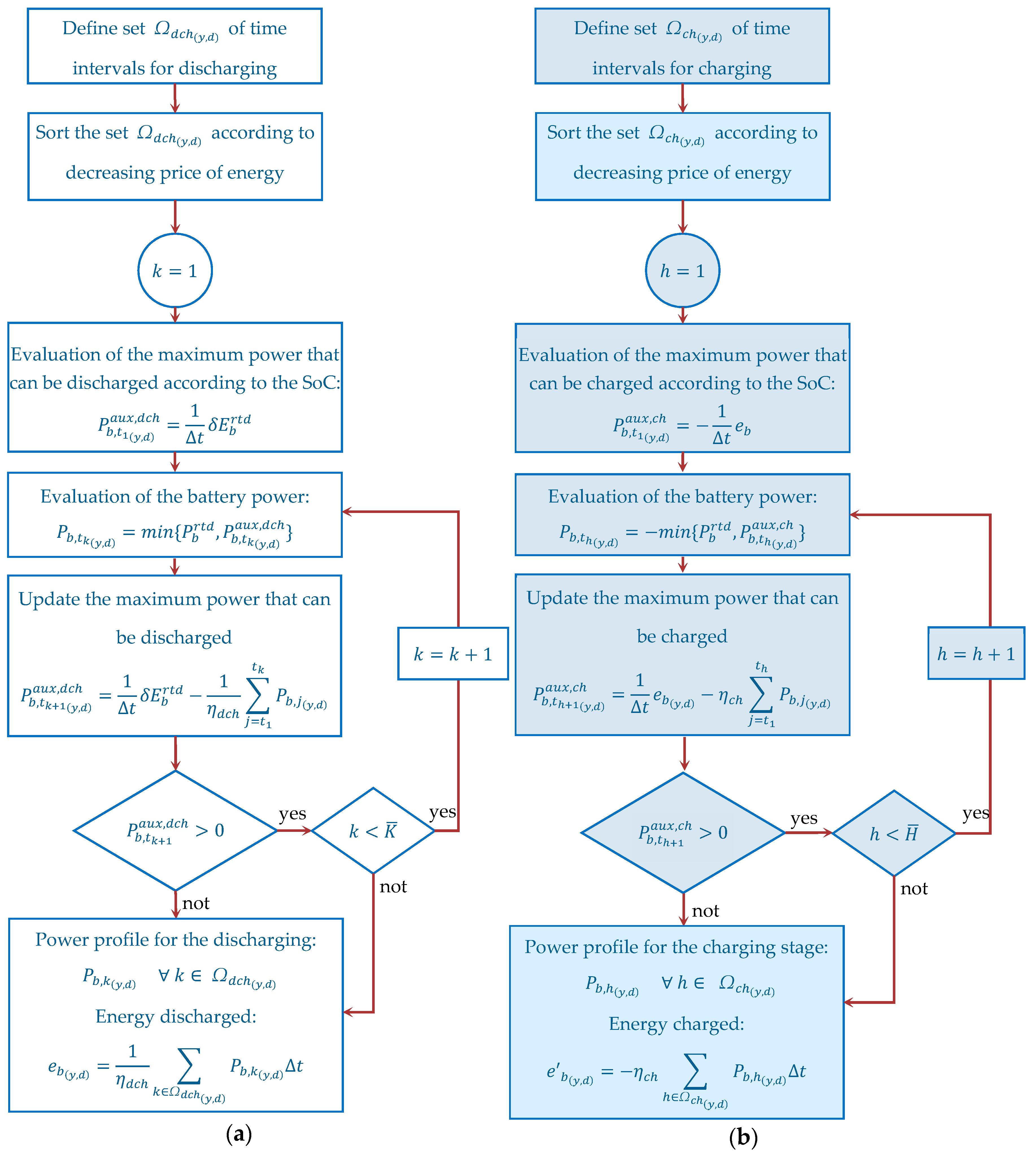
Figure 3.
The microgrid under study.

Figure 4.
Load profile at bus #6.

Figure 5.
PV power profile at bus #15.
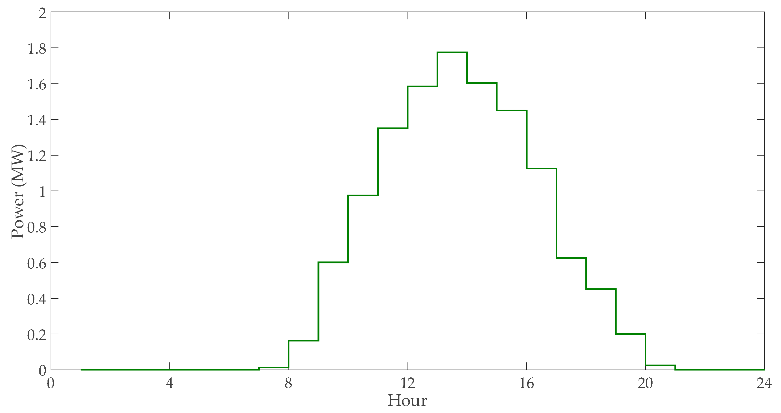
Figure 6.
Market energy price (data taken from [36]).
Figure 6.
Market energy price (data taken from [36]).
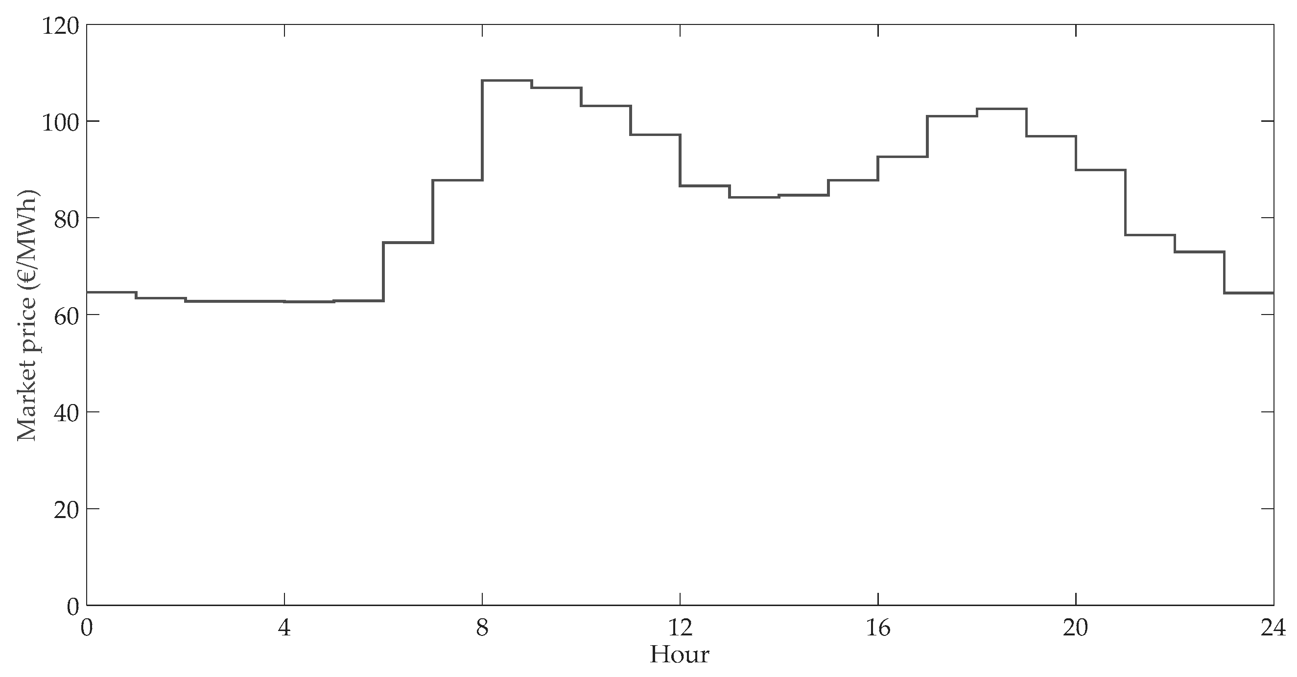
Figure 7.
Active power of the EESS connected at the bus #6 (case study 1).
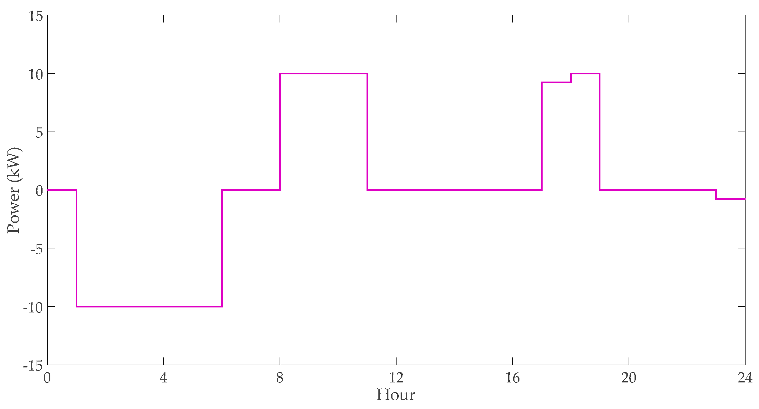
Figure 8.
Voltage values along a day of the first year of the planning period at the bus where EESS (bus #6) and PV unit (bus #16) are connected (case study 1).
Figure 8.
Voltage values along a day of the first year of the planning period at the bus where EESS (bus #6) and PV unit (bus #16) are connected (case study 1).
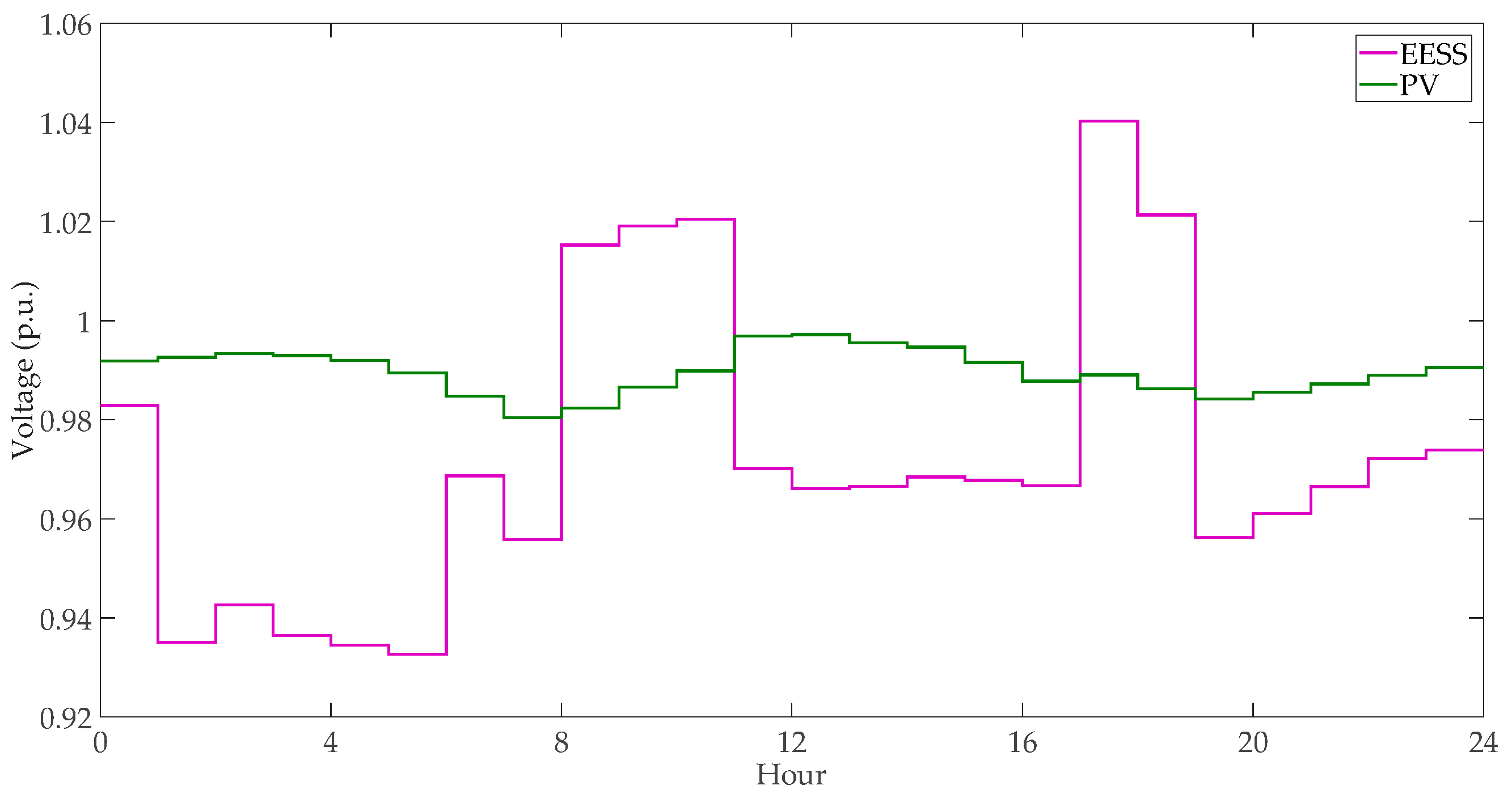
Figure 9.
Active power imported from the whole µG along a day of the first year of the planning period.
Figure 9.
Active power imported from the whole µG along a day of the first year of the planning period.


Table 1.
Annual Average Voltage Dip Number for MV substations connected to the Italian National Grid (data taken from [34]).
Table 1.
Annual Average Voltage Dip Number for MV substations connected to the Italian National Grid (data taken from [34]).
| Residual Voltage [%] | Annual Average Voltage Dip Number | ||||
|---|---|---|---|---|---|
| Duration of the Voltage Dips [ms] | |||||
| 20–200 | 200–500 | 0.5–1 × 10³ | 1–5 × 10³ | 5–60 × 103 | |
| 80 ≤ u ≤ 90 | 33.93 | 4.35 | 0.93 | 0.34 | 0.05 |
| 70 ≤ u ≤ 80 | 12.91 | 3.01 | 0.38 | 0.21 | 0.07 |
| 40 ≤ u ≤ 70 | 17.07 | 3.95 | 0.31 | 0.11 | 0.03 |
| 5 ≤ u ≤ 40 | 5.22 | 1.39 | 0.12 | 0.02 | 0.00 |
| 1 ≤ u ≤ 5 | 0.27 | 0.05 | 0.07 | 0.03 | 0.10 |
| Total | 69.4 | 12.74 | 1.82 | 0.72 | 0.25 |
Table 2.
Load Input data.
| Bus # | Rated Power (MVA) | Load Type | cos φ | Bus # | Rated Power (MVA) | Load Type | cos φ |
|---|---|---|---|---|---|---|---|
| 2 | 13.8 | Residential | 0.93 | 8 | 0.30 | Comm./industrial | 0.95 |
| 9.16 | Comm./industrial | 0.87 | 9 | 0.25 | Residential | 0.90 | |
| 3 | 0.35 | Residential | 0.95 | 0.20 | Comm./industrial | 0.90 | |
| 0.80 | Comm./industrial | 0.85 | 10 | 0.35 | Residential | 0.95 | |
| 4 | 0.25 | Residential | 0.90 | 11 | 0.50 | Residential | 0.90 |
| 0.24 | Comm./industrial | 0.80 | 12 | 0.10 | Residential | 0.95 | |
| 5 | 0.40 | Residential | 0.90 | 0.45 | Comm./industrial | 0.85 | |
| 6 | 0.20 | Residential | 0.95 | 13 | 3.20 | Residential | 0.90 |
| 0.30 | Comm./industrial | 0.85 | 3.78 | Comm./industrial | 0.87 | ||
| 7 | 0.15 | Residential | 0.95 | 14 | 0.68 | Comm./industrial | 0.85 |
| 8 | 0.10 | Residential | 0.95 | 15 | 0.27 | Comm./industrial | 0.90 |
Table 3.
EESS Data (data taken from [37]).
Table 3.
EESS Data (data taken from [37]).
| Parameter | Value | Parameter | Value |
|---|---|---|---|
| Battery round trip efficiency | 99 % | Battery Cycle life | 4800 cycles |
| Maximum Depth of Discharge | 100 % | Converter round trip efficiency | 98 % |
| Battery installation cost | 153 $/kWh | Converter installation cost | 59.6 $/kW |
| Battery replacement cost | 110 $/kWh | Maintenance cost | 1.5% |
Table 4.
Candidate buses (70% threshold values).
| Case Study | |||||
|---|---|---|---|---|---|
| Case 1 | Case 2 | Case 3 | Case 4 | Case 5 | Case 6 |
| 3 | 6 | 8 | 3 | 3 | 8 |
| 4 | 7 | 9 | 4 | 4 | 9 |
| 5 | 8 | 10 | 5 | 5 | 10 |
| 6 | 9 | 11 | 6 | 6 | 11 |
Table 5.
Siting and sizing of EESSs.
| Case Study | Accounting for Voltage Dip Costs | BF (M$) | Voltage Dip Cost Reduction (M$) | EESSs’ Nodes | EESSs’ Sizes (MW) | ||
|---|---|---|---|---|---|---|---|
| EESS n. 1 | EESS n. 2 | EESS n. 1 | EESS n. 2 | ||||
| 1 | Yes | 4.81 | 1.63 | 3 | 6 | 10 | 10 |
| No | 3.19 | - | 3 | 6 | 10 | 10 | |
| 2 | Yes | −0.16 | 0.44 | 6 | - | 5 | - |
| No | −0.59 | - | 9 | - | 5 | - | |
| 3 | Yes | −0.34 | 0.31 | 9 | - | 5 | - |
| No | −0.65 | - | 9 | - | 5 | - | |
| 4 | Yes | 4.75 | 1.63 | 3 | 6 | 10 | 10 |
| No | 3.16 | - | 3 | 4 | 15 | 5 | |
| 5 | Yes | 4.70 | 1.63 | 3 | 6 | 10 | 10 |
| No | 3.21 | - | 3 | 5 | 5 | 15 | |
| 6 | Yes | 4.46 | 0.50 | 8 | 10 | 15 | 10 |
| No | 3.96 | - | 8 | 10 | 15 | 10 | |
Table 6.
Benefit corresponding to the voltage dip cost reductions.
| Case Study | Percentage Value of the Voltage Dip Cost Reduction on the Total Benefit (%) | Percentage of Value of the Voltage Dip Cost Reduction on the Installation and Replacement Cost (%) |
|---|---|---|
| 1 | 33.89 | 6.55 |
| 4 | 34.32 | 6.55 |
| 5 | 34.68 | 6.55 |
| 6 | 11.21 | 1.61 |
© 2020 by the authors. Licensee MDPI, Basel, Switzerland. This article is an open access article distributed under the terms and conditions of the Creative Commons Attribution (CC BY) license (http://creativecommons.org/licenses/by/4.0/).
Share and Cite
MDPI and ACS Style
Mottola, F.; Proto, D.; Varilone, P.; Verde, P. Planning of Distributed Energy Storage Systems in μGrids Accounting for Voltage Dips. Energies 2020, 13, 401. https://doi.org/10.3390/en13020401
AMA Style
Mottola F, Proto D, Varilone P, Verde P. Planning of Distributed Energy Storage Systems in μGrids Accounting for Voltage Dips. Energies. 2020; 13(2):401. https://doi.org/10.3390/en13020401
Chicago/Turabian StyleMottola, Fabio, Daniela Proto, Pietro Varilone, and Paola Verde. 2020. "Planning of Distributed Energy Storage Systems in μGrids Accounting for Voltage Dips" Energies 13, no. 2: 401. https://doi.org/10.3390/en13020401
Note that from the first issue of 2016, this journal uses article numbers instead of page numbers. See further details here.