1. Introduction
The share of renewable power generation in the global electricity generation is anticipated to expand from today’s 23% to levels between 30%–45% by 2030 [
1]. This technological alteration requires a rethinking in the way power systems are planned, maximize the benefits from renewables affordably and securely. Since renewable energy integration brings new challenges into the distribution network planning an accurate planning model, which incorporates system uncertainty introduced by renewable resources and loads, is necessary for making planning decision.
The technological development of large-scale electrochemical energy storage system (ESS) has resulted in capital cost reductions and increased roundtrip efficiency enables them to become a feasible option to deploy in the distribution network [
2,
3]. Storage applications such as energy arbitrage [
4], peak shaving [
5], frequency regulation [
6], voltage support [
7], and congestion management [
8] have made it vital to integrate more ESS in the distribution network. Thus, optimal planning and management of ESS are essential to identify ideal configurations. However, many of the optimization algorithms proposed in recent literature do not adequately deal with uncertainties. For instance, the real amount and position of distributed generation (DG) that is going to be connected to the system, the mix of renewable energy sources (RES), the cost of ESS or the level of participation and the cost for active demand [
9].
Sizing of ESSs in distribution networks from DSO has been discussed in [
10]. The number and locations of the ESSs are assumed to be given. An AC-optimal power flow (AC-OPF) with semidefinite programming (SDP) convex relaxation is adopted for network simulation. To consider uncertainties in the model, a stochastic optimization approach has been considered. Two different problems have been formulated respectively for the siting and sizing of ESS in distribution networks coupled with a wind farm in [
11]. However, the authors considered a linearized DC-optimal power flow (DC-OPF), and the wind power forecast is assumed perfect. Apart from siting and operation, the authors of [
12] suggest the life cycle payment of storage. They present two models for a transmission-constrained power network with storage. Both models use a DC-OPF framework. The first model selects optimal siting and operation of the storage assuming a fixed group of different storage technologies. The second model expands the DC-OPF framework to optimize the storage technology mix, new storage capacity investments, and the network allocation of these resources. The authors of [
13] provide a mathematical model that simultaneously optimizes transmission switching operations, ESS siting and sizing decisions and taking into account the limits on maximum allowable load shedding and renewable energy curtailment amounts in the power system. The methodology proposed in [
4], based on a linearized DC-OPF, captured both the monetary and technical advantages of investment in storage and adopted a sensitivity analysis to assess the impact of uncertain parameters. As opposed to an analytical approach, the authors of [
14] detail a heuristic approach for finding the optimal location(s) and size of a multi-purpose ESS including transmission and distribution parts without considering the uncertainty in the model. In the transmission storage part, a sensitivity analysis is performed using complex-valued neural networks (CVNN) and time domain power flow (TDPF) to obtain the optimal ESS location(s). In [
15] a multi-criteria approach where a genetic algorithm (NSGA-II) has been used to identify the optimal place, size, and scheduling of energy storage in the distribution network. The authors created a full multi-objective (MO) optimization procedure able to identify the Pareto set of design options with fixed network topology for a given medium voltage (MV) network. In addition to that, the same authors of [
15] have proposed a multi-criteria analysis approach selecting the best planning alternative for energy storage integration in the distribution system [
16]. However, heuristic techniques often required a high computational burden and are not guaranteed to converge in global optima [
17].
Convex relaxation techniques have been developed to obtain an acceptable solution while ensuring algorithmic efficiency. The two most commonly used relaxations for distribution network are semi-definite program (SDP) and second-order cone programming (SOCP). Though both SOCP and SDP have been proven exact under certain conditions [
18,
19]. In this paper, SOCP has been adopted due to its higher algorithmic performances that imply fast convergence to global optima and to reduce the heavy computation cost.
The current literature on energy storage study is divided into three classifications: (i) storage sizing, (ii) storage operation, and (iii) storage siting. Less publications exist about the optimal location(s) of the ESS than publications on optimal sizing likely due to the difficulty of finding optimal sites [
20,
21]. Storage siting is the least researched and most complicated of these three classifications. The optimal operation studies of ESS consider that energy and power ratings of a storage unit are given, the purpose of these studies is to identify operation strategies to optimize the exploitation of resources able of contributing to network support at minimum cost. These studies typically do not address network constraints. The optimal ESS size (i.e., energy and power ratings) depends on the state at which the storage is optimally operated [
22]. In turn, optimal storage siting depends on the amount of the storage being considered and how it will be controlled. This problem becomes even more complicated when it considers distributed storage rather than a single storage unit. If this is the case, the amount of storage located is typically undefined at first. ESSs are considered one of the solutions to manage the DG downsides and to help incorporate RES in the distribution networks, which rely largely on the flexibility of resources [
23,
24].
Capital intensity is the main barrier to the deployment of ESS [
25]. Investment in the ESS, therefore, requires a trade-off between long-term investment costs, short-term operating conditions, and the benefits that these services will offer. It includes optimizing their network position (i.e., location) and operating parameters (e.g., size and operating profile) simultaneously [
26]. The objective of the optimization is generally multiple since it spans from the reduction of CAPEX (Capital Expenditures) for network upgrade to the reduction of energy loss costs as well as power quality costs [
27]. RES and electric vehicles (EVs) integration as well as the engagement of customers in flexibility programs are opening new opportunities for ESS and making clear the need for optimal siting and sizing methodologies [
28].
ESS technologies can operate on different timescales, ranging from seconds to hours. The services offered by ESS can be divided into power- and energy-related services, based on the timescale of interest [
29]. Transient stability and ancillary services, such as frequency regulation, spinning reserve, and voltage control are power-related services. Back-up power provision, black-start, uninterruptible power supply (UPS), standing reserve, and seasonal energy storage are typical examples of energy-related services [
28,
30]. Both ESS owners and other system stakeholders can benefit from the provision or the usage of these services.
The ESS optimal positioning and sizing problem aims at the maximization of the benefit-cost ratio subject to the non-linear/non-convex network constraints that make the solution more cumbersome and requires specific mathematical tool [
31]. The research on the topic has been dramatically increasing in the last two years since ESS are crucial for the energy transition towards the carbon free world, but there is still room for new contributions, particularly on dealing with the uncertainties modeling.
For these reasons, the paper proposes an application of the Robust Optimization (RO) to solve the ESS optimal location problem in distribution networks operated by a DSO. The objective of the optimization problem is to use ESS for delivering power without any violation of technical limits (e.g., maximum and minimum nodal voltage), minimizing the resort to RES or combined heat and power (CHP) generation curtailment and load shaving. Indeed, the DSO can evaluate the ESS installation as a non-network option to avoid the expensive and time consuming building or revamping of networks, particularly in the current situation of limited markets of services offered by customers or other producers. However, the convenience to do this strictly depends on the site, size, and operation of the ESS, that in turn, depend on the state of the network, that is intrinsically uncertain. The approach proposed in the paper deals with the uncertainties with an original implementation of the Robust Optimization. The algorithm has been validated with an exemplary distribution network representative of one class of the Italian distribution classes of networks produced by the project ATLANTIDE (Archivio TeLemAtico per il riferimento Nazionale di reTI di Distribuzione Elettrica” that means “Digital archive for the national electrical distribution reference networks”) [
32].
The paper is organized as follows:
Section 2 describes the detailed formulation of energy storage placement problem.
Section 3 discusses the uncertainty modeling approach.
Section 4 describes the solution methodology of a robust optimization problem.
Section 5 and
Section 6 present the case study with real data and conclusion, respectively. Finally, in the nomenclature of the symbols used in the mathematical formulation has been reported.
2. Deterministic Formulation of Energy Storage Planning
The objective function (OF) of the deterministic model consists of minimizing the operational extra-cost that should be sustained for complying with the technical constraints. Such cost includes the penalty terms for RES (
) and biomass CHP generation curtailment (
), and the cost of shaving the peak loads (
). Furthermore, since the goal of the paper is to evaluate the contribution of energy storages to the management of the network, even in uncertain conditions, the investment cost
to be sustained for the storage allocated in the network is added to the operational cost, as in (1).
This minimization is subject to voltage and current limits, power flow equations, and storage technical constraints. In the following, each cost term and constraints are detailed.
2.1. Penalty for RES Curtailment
To strongly penalize the generation curtailment of RES, the cost of curtailed energy due to network constraint violations has been monetized as twice the price of energy paid in the wholesale market
cEN (here, 58 €/MWh, according to the average Italian energy selling price) [
33], as in (2).
where
is the energy curtailed at the time interval
t by the RES generator connected to the
n-th bus of the network.
Since the increment of the network hosting capacity may be quantified via the possibly avoided curtailment of RES production, the smaller this term, the better the storage allocation solution.
2.2. Penalty for Biomass CHP Curtailment
This cost for biomass CHP curtailment is assumed proportional to the avoided cost for fuel saving
F [€/MWh], increased by 20%. The fuel cost
F has been considered here equal to 80 €/MWh, by assuming the average gas price ≈ 35 c€/m
3 ≈ 36 €/MWh
t and by hypothesizing an efficiency for the electric conversion about 45%. This assumption allows penalizing also the CHP curtailments, with high cost, as in (3).
where
is the energy curtailed at the time interval
t by the biomass CHP connected to the
n-th bus of the network.
2.3. Peak Load Shaving Cost
Regarding the term referred to the active customers, in this paper only the cost of shaving the peak loads has been considered, by assuming that it is not possible to fully control the customer demand but only cut a quote of their consumption in some critical conditions. It is assumed, as the RES curtailment, that this curtailed energy is paid at twice the energy price
to penalize load curtailment with the higher cost, as renewable generation curtailment, according to (4).
where
is the energy curtailed at the time interval
t to the customer connected to the
n-th bus of the network.
2.4. Storage Investment Cost
The storage investment cost (
) is a function of the size of the storage in terms of rated power and energy as in (5).
where
cP and
cE are the specific costs of the ESS adopted technology, reliant respectively on the power rating
and the nominal capacity
of the
n-th ESS located in the network (here
cP = 200 €/kW and
cE = 400 €/kWh, according to the market cost of lithium-ion technology [
15]).
To consider this cost in the objective function (1), only a daily quote of
SCn is added to the operational terms of (1), calculated as in (6).
where
Ks is a capital recovery factor (here
Ks = 0.1, for considering 10 years as ESS lifetime).
In this paper, it is assumed that the storages are DSO owned and managed for relieving contingencies. Thus, the ESS OPEX (operational expenditures) is not considered in the optimization. According to this point of view, it is supposed that the minimization of the network operational cost, in terms of reduction of the curtailed power from RES and to loads, that would be necessary to relieve contingencies, represents the only incomes that allow DSO to pay back EES CAPEX (capital expenditures) and ESS OPEX. The depreciation of the ESSs is assumed negligible and not added to the ESS cost term.
2.5. Load Balancing Constraints
The SOCP convex relaxation has been used in the proposed multi-temporal AC-OPF model.
Equations (7) and (8) are the nodal active and reactive power balance.
where
and
define the expected RES and CHP production in terms of active and reactive powers,
and
are the active and reactive power delivered to the load connected to the
n-th node,
and
are respectively the current, the active and the reactive power flowing in the branch from the
m-th bus to the
n-th one,
and
are the resistance and reactance of the
mn-th branch.
and
are the charging and discharging power of the storage at time
t.
and
are the active and reactive power provided by the upstream connections (slack bus of the network). The values of
and
are zero except for the first node.
2.6. Network Constraints
The current magnitude quadratic term can be defined as the function of the corresponding active and reactive power quadratic terms (Equations (9)–(11)).
Equation (9) is relaxed ultimately by relaxing the magnitude of currents within each branch and using a conic formation on the limitation of exchanged active power. For linearization purposes, the quadratic terms of voltage and current magnitude have been replaced with the linear ones as in (12).
The new variables (
,
) successfully formulate the SOCP problem according to the following constraint,
The Equation (13) provides the voltage limits of each bus.
Bus 1 is modelled as a swing bus with fixed complex voltage .
2.7. Constraints for RES and Controllable Generator
Equations (14) and (15) impose the limits to the active and reactive power curtailment associated with RES and CHP generators. In Equation (14),
represents the lower bound of the active power curtailment of RES and CHP generators. In this study, the lower bound value of curtailment has been chosen as 0, which means the generators curtail all of their capacity. The upper bound,
, has been considered the capacity of the generators based on the expected values of each time step.
Furthermore, the constraints about storages may be formulated as in (16)–(20).
where
ϵ [0 or 1] and
ϵ [0 or 1].
The state of charge (SoC) of ESSs is calculated by considering the initial SoC and the charging and discharging efficiencies
and
(Equation (16)). To restrict the maximum charging and the depth of discharging and for avoiding the simultaneous charging and discharging, the binary variables
and
, of which only one can be different from zero, have been considered in Equations (17)–(20). Finally, Equation (21) is added to force the SoC to be equal at the beginning and the end of the considered time horizon
T.
The multiplication of binary and integer variables during the estimation of the charging and discharging power of the storage unit generates a quadratic term. A decomposition technique has been used to linearize the relevant constraints by rewriting constraints in the form of (22) as in (23) and (24) to avoid the bilinear terms.
and are continuous, binary, integer. The continuous and integer variables are respectively variable in [0, zmax].
3. Uncertainty Management
Uncertainties are mostly involved in decision-making problems. The uncertainty from electric loads, wind, and solar power generation typically influence distribution planning in general and storage allocation in particular. Several factors determine the evolution of each uncertainty. For example, the consumers’ activities, energy savings and electricity providers’ rate policies influence the electric load; the radiation of the sun and the velocity of air impact on the power output of PV and wind [
34].
A static robust optimization is used to consider the uncertainty in the optimal planning model. To define the uncertainty set, an interval uncertainty model has been adopted with the flexibility to regulate the robustness, called budget of uncertainty (. Static robust optimization devising seeks for optimal solutions that optimize the objective function and encounter the problem requirements for every possible revealing of the uncertainty in constraint coefficients. Hence, the variables are independent of the uncertain parameters.
For a worst-case analysis, when considering the uncertainty, the following problem (25)–(27) is dealt with:
In the above optimization problem, Equations (25) and (26) represent the objective function and inequality constraint, respectively. The uncertainty bound of the uncertain parameter that must assume values between lower l and upper u bounds, as formulated by the Equation (27). is the value of the right-hand side of i-th constraint.
For the
i-th constraint, the auxiliary problem can be formulated as follows:
To make the model tractable, that means to convert the inner maximization problem to a minimization problem, the dual of the above problem (28)–(30) needs to be formulated as follows:
Subject to
where
,
are the dual decision variables for constraints of the auxiliary problem.
Incorporating model (31)–(34) into the original problem (25)–(27), the robust linear counterpart is formulated as:
4. Robust Counterpart
Assume that all the decision variables should be considered before the revealing of the uncertainty from solar power, wind generation, and electric loads. In the active power balance (7), uncertainties
and
are modeled as symmetric and bounded variables
,
. It should be mentioned here that
consists of the solar and wind generations. The uncertainty takes values as in the following Equations (41)–(43).
In the robust model, the objective function (1) is identical to the deterministic model. The only constraint that is affected by uncertainty is the electric power balance equation. The electric power in the network should be met when the worst case of uncertainties occurs. For the power balance equation, the worst case would occur at the maximum increase of the electric loads and the maximum decrease in solar (PV) and wind power generation. Therefore, the robust formulation becomes as in (44)–(47).
Subject to
where
are the scaled deviations from the random electric loads, solar, and wind power generation, respectively.
is the budget of the uncertainty of uncertain parameters at time
t that lies between 0 to 1, where 0 being the deterministic case and 1 defined the most robust case.
To make tractable the above problem, the following subproblem in Equations (48)–(50) need to be formulated into the corresponding dual problem by introducing dual variables , for constraints (49) and (50).
The subproblem can be formulated as in (48).
The robust counterpart after applying the duality theory is formulated as in (51)–(55).
Finally, the tractable robust model can be formulated as the following (56) and (57).
Moreover, the constraints (8)–(21) and (52)–(55) form the tractable problem.
The new model does not contain any uncertainty and is formulated as a mixed-integer second-order conic programming (MISOCP) problem that can be solved efficiently using CPLEX that uses a branch and cut algorithm to find the integer feasible solution.
5. Case Study
The procedure was applied to a test distribution network derived from the ATLANTIDE project [
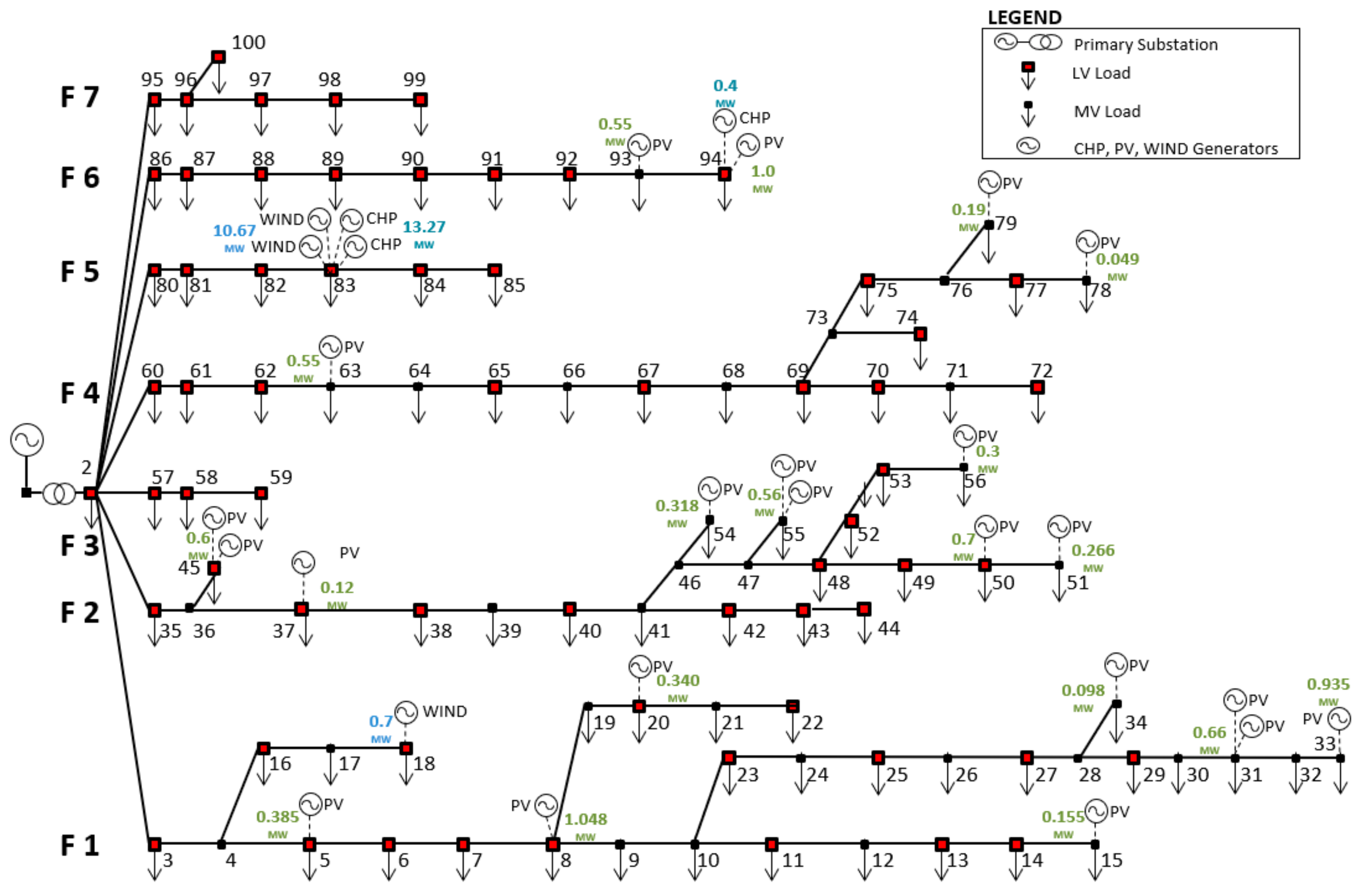
32]. The MV network, shown in
Figure 1, representative of the industrial ambit, was constituted by 100 nodes, subdivided in seven feeders supplied by a primary substation equipped with a 25 MVA high voltage/medium voltage (HV/MV) transformer. The total demand was about 30 MVA (372 GWh/year) and the total installed DG capacity was 34 MW (27.2 GWh/year), as a mix of wind, PV and biomass CHP generators.
The mathematical formulation of the RO for an AC-OPF based energy storage planning tool was programmed in General Algebraic Modeling System (GAMS) (GAMS Software GmbH, Frechen, Germany) and solved using CPLEX 25.1.1 on a 2.30 GHz personal computer with 4 GB RAM. In this experimental study, the worst case was considered when the load was high ( = 1) and wind and PV generation was low ( = −1).
For the sake of a comprehensive view, in the following, the results obtained by the application of the described optimization to the network of
Figure 1 in 12 typical days, differentiated between working days, Saturdays, and holidays (Sundays included), and between seasons, have been reported. The time horizon of 24 h of each typical day has been considered with a time step of 1 h. Three scenarios have been considered: the certain one (solved by the deterministic OPF) and two uncertain scenarios with different values of risk (
and
), both solved with RO. Furthermore, for highlighting the advantages provided by the storage systems the case of deterministic optimization (certain) without storage has been added to the previously described cases.
All the buses of the test network were assumed candidates for storage placement. The available ESS were considered of 1.0 MW/2 h storage capacity. The efficiencies for charging and discharging were considered 90% each, which gives an overall roundtrip efficiency of 0.81. The initial state of charge (SoC) has been considered 25% of its capacity.
In these typical days, some under-voltage conditions occur in the most distant nodes from the HV/MV transformer and, thus, for solving these issues, it is necessary to resort to the load peak shaving. Furthermore, some lines suffer for overloading depending on the non-coincidence of load demand and DG production. ESSs prove to be useful for reducing the curtailment of the demand and production as detailed in the next subsections.
5.1. Generation and Load Profiles
The generation and load profiles were simulated according to the ATLANTIDE load and generation daily curves, that provide for different kinds of customers (i.e., industrial, residential, commercial, and agricultural) and for several technologies of DG (i.e., wind turbine, PV, and CHP biomass-based) the hourly consumption/production for each typical day. An amount of 22 PV systems was assigned to 20 nodes. The size of these systems is between 49–1048 kW. Node 8 had the biggest PV system, whereas the lowest one was connected to node 78. Node 83 comprised two wind generators and two CHP plants.
Figure 1 depicts the nominal power of the PV, wind, and CHP of each node.
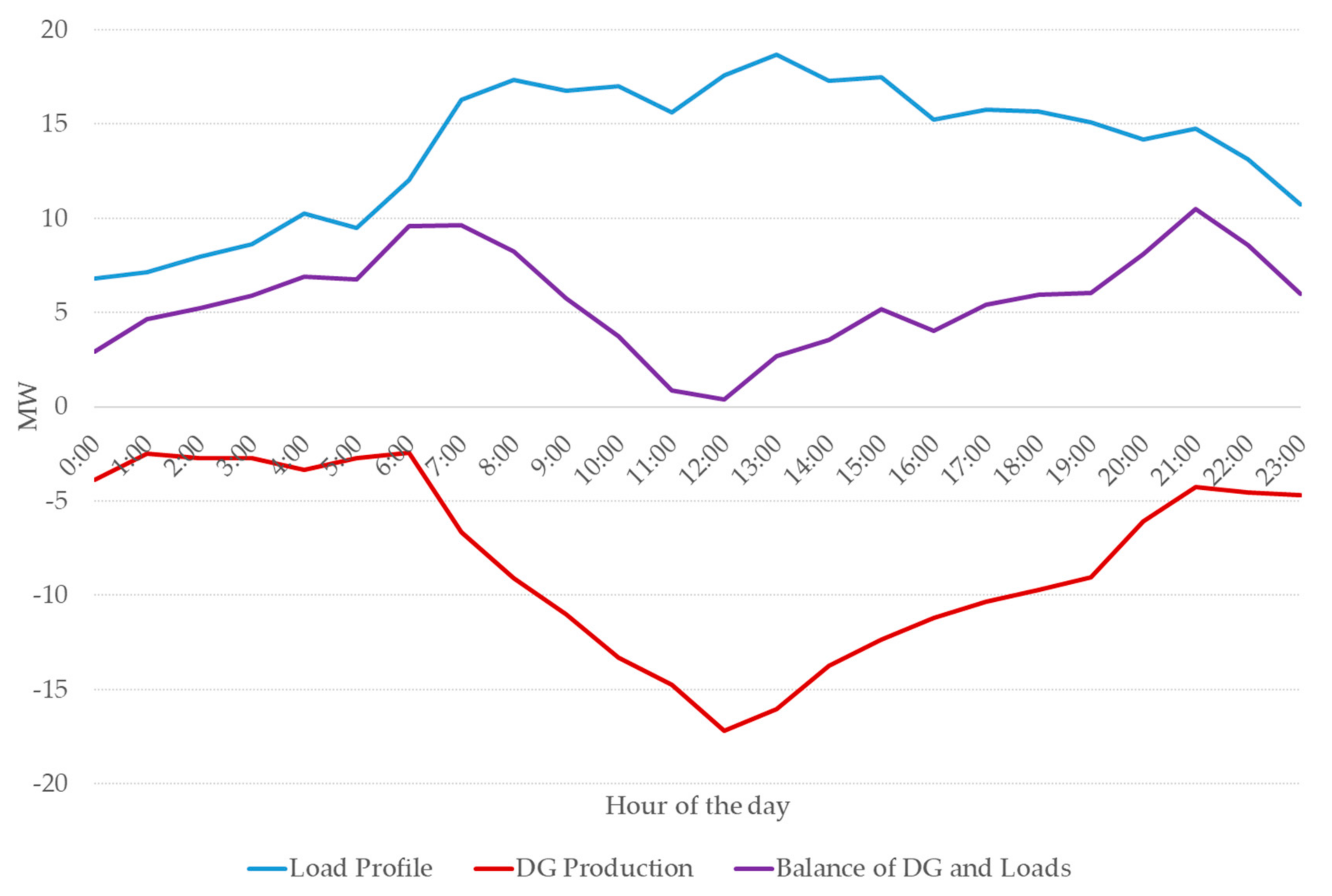
The load profiles indicated a peak load of 18.69 MW during the spring working day and 18.14 MW during the summer working day with an average load of 13.79 MW and 13.38 MW, respectively. As an example, the demand and production profiles and their balance at the HV/MV interface, during the spring working day, are shown in
Figure 2.
5.2. Storage Placement
The optimization results of storage position for each typical day for the three considered cases have been enumerated in
Table 1. The ESS optimal positions may change from one typical day to another even for the same case, but the results can be summarized by considering a given solution valid for all the twelve typical days. In the following, it has been assumed that the placement in one bus or a close one on two different typical days can be considered the same placement. For instance, the bus 83 and the bus 84 in the deterministic case, that are the solutions for the TD8, and the TD5 respectively, can be considered as a unique optimal position around the bus 83.
On the contrary, if two busses, even close, appeared in the solution of the same day they were both considered necessary and two ESSs had to be placed on that nodes (e.g., the busses 83 and 85 in the results of all the cases for the TD12 or the busses 83 and 84 in the results of the intermediate and robust cases for the TD5). By applying these rules, the total number of ESSs that had to be placed in the three cases are reported in the last row of
Table 1. It is worthy of mentioning that the results were substantially incremental: the intermediate case included the location of the deterministic case, and the robust case (no risk) included, in turn, the intermediate one.
To analyze the impact of renewables and load uncertainty on the investment of the energy storage in the distribution network, one of the worst-cases of RES (PV, wind or biomass based) and combination of loads were considered. The worst-case scenario considered in this work was when the loads had upper bound values, and the renewables had lower bound values. Three cases were considered by varying the loads and renewables uncertainty bounds. In the first case, the budget of uncertainty was zero (), i.e., the profiles of load and renewable generations were assumed following the forecasted values. In the second case, the value of budget of uncertainty for both load and renewables considered 0.5 () that is between the zero (deterministic) and 1 (robust or worst case). In the third case (), the considered worst-case scenario was evaluated. In this case, the uncertainty sets of loads and renewables were considered broader to consider the possible extreme coordinates of the uncertainty set.
The following figures compare the results of the studied cases (i.e., no control, deterministic OPF no storage, deterministic OPF with storage, intermediate and robust). These results are related to the most critical typical day, the winter working day (TD1). For the sake of clarity, the figures refer only to the feeder F1 that is the longest feeder of the test network depicted in
Figure 1 (i.e., the last bus is about 14.2 km far from the primary substation).
Figure 3 shows the voltage profiles occurring at 9:00 am of the winter working typical day, because, among other time intervals, this one was proved that experiments the greatest load curtailment;
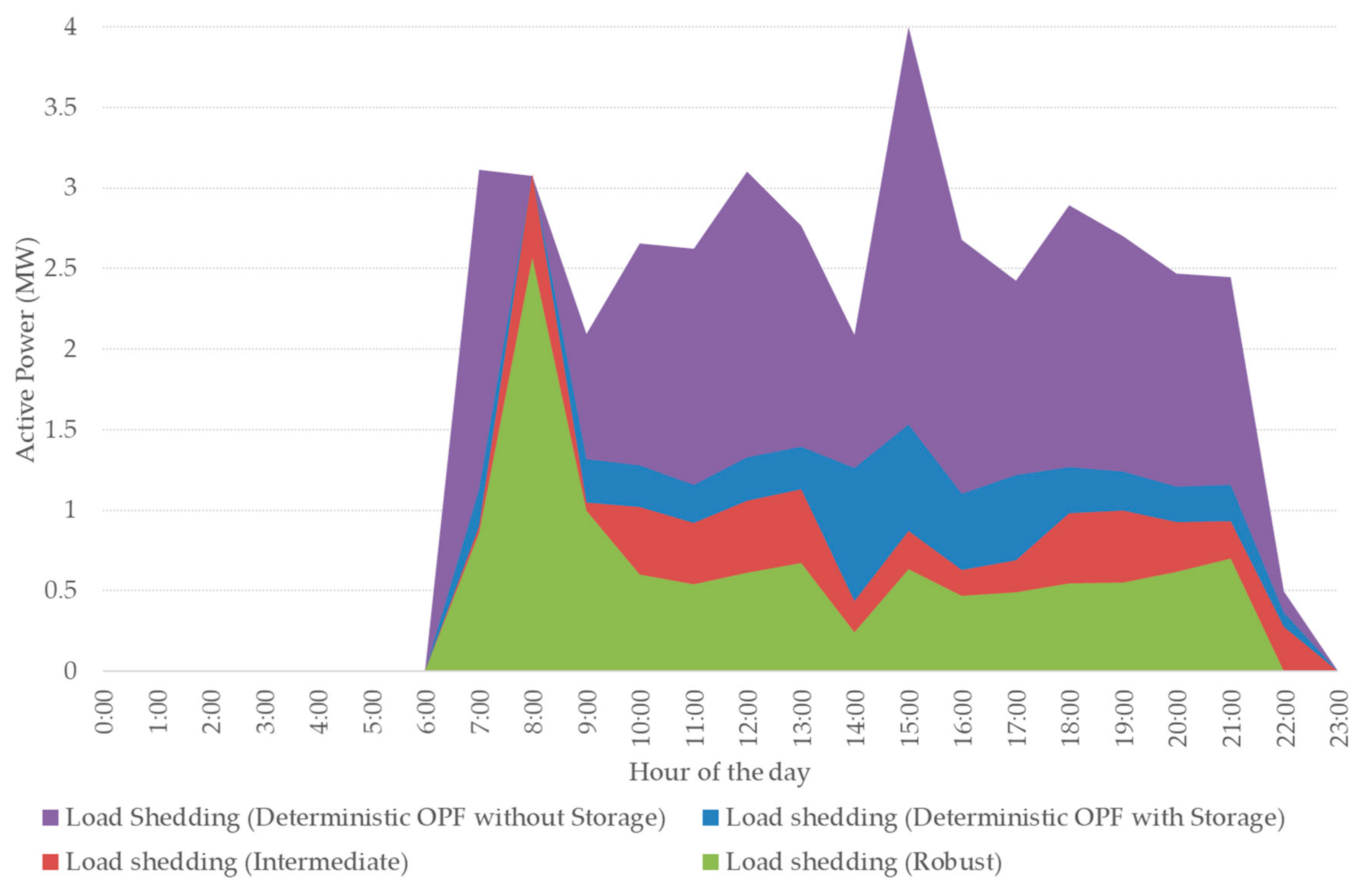
Figure 4 shows the load curtailed during this typical day, in
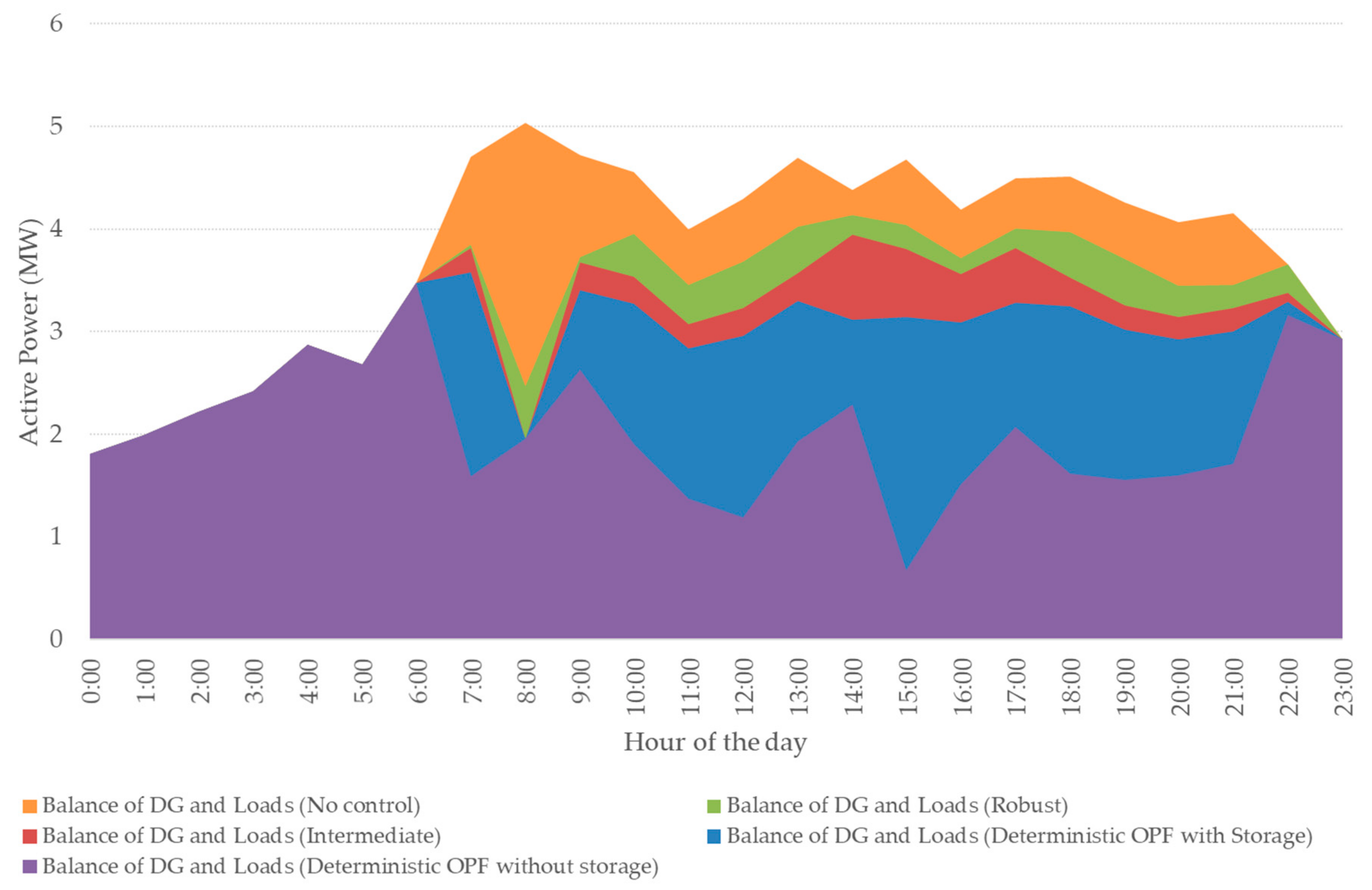
Figure 5 the balances of DG production and curtailed demand, and, finally,
Figure 6 the ESS charging/discharging optimal profiles of one of the ESS optimal positioned in the feeder F1 (bus 10 of
Figure 1). As it is evident by the results, all the optimizations allow to solve the undervoltage conditions occurring in the long feeder F1 (
Figure 3); the more conservative the optimization (i.e., by moving from certain to uncertain, intermediate and robust, optimization) the smaller the demand curtailed (
Figure 4); in the feeder F1 no generation curtailment results from the optimizations, thus the balance of production and demand (curtailed) is closer to the original one (no control) in the robust case (
Figure 5). It is worth noticing that the voltage value at the sending end (the MV busbar of the primary substation) was lower in the no control case than the other cases because the implemented model of the HV/MV transformer is very simple and strongly suffers for the high demand, not curtailed in the control case. In future works, the transformer model will be improved. These results, together with the ESS operation, are discussed more in detail in the next subsections for each optimization case.
5.3. Deterministic Case (with and without Storage)
Due to the absence of uncertainty, in this case, the load and renewables profiles will remain the same as the predicted values. It was witnessed that during the deterministic case with storage, at least four storages need to cover their requirements. The ESS optimal positions can change from one typical day to another, but, by summarizing the results in the 12 typical days (
Table 1), they were located two in the two lateral branches that start from the node 10 (feeder F1, positions are 10 or 12 and 32). The third and fourth ESS had to be located around the node 83 (feeder F5, positions are two among 83, 84 and 85). It is essential to observe that node 83 is the node that had the highest number of renewables and CHP connected; thus, it is noticeable to consider that as a privileged position for storages.
The highest load curtailment was experienced during the typical day of winter working day (TD1) with the amount of 51.77 MWh/day for the case without storage and 30.46 MWh/day for the case with storage.
By focusing on the feeder F1, as it is evident from
Figure 3, the nodes of this feeder had under-voltage issues in the no control case, and any optimization forces to resort load shedding (
Figure 4). By comparing these two certain cases, is it worth noticing that if the ESSs are not available for the optimization (deterministic OPF no storage) much more demand had to be curtailed (i.e., 41.62 MWh/day of the no storage case vs. 20.97 MWh/day in the case with storage).
The daily operation of the ESS was optimized as well as the optimal position. For instance, during the winter working day, the daily operation profile of the ESS located around bus 10 is shown in
Figure 6, together with the balances of demand and production curves, with and without ESS. At the beginning of the day, the ESS started to charge, keeping the final balance of demand, DG production (minimal in the first hours of the day), and charging power for ESS so low to do not negatively impact the network operation. At around 7:00 am, when the morning peak starts, the storage discharges for reducing the power demand and keeping the voltage profile within the limit (
Figure 3).
5.4. Intermediate Case
In this case, a narrow uncertainty bound is considered. The budget of uncertainty for the uncertain parameters has been considered as
. The optimization algorithm will look for a solution inside the specified uncertainty bound. From
Table 1, by considering the simulation results of the twelve typical days, and assuming the most conservative hypotheses (i.e., the final result is the union of the results obtained for each typical day), the intermediate case suggests at least five storage systems to be installed: two in the feeder F1 and two in the feeder F5, as in the deterministic case, plus one ESS in the feeder F4. The positions of the two storages in the feeder F1 and the two in the feeder F5 are more or less the same of the deterministic case (F1 possible locations are the busses 10 or 12 for one lateral and the busses 27, 32, or 34 for the other lateral, and two positions among the bus 83, 84 or 85 for the feeder F5). In the feeder F4, the added storage system has to be installed around the node 77.
The load shedding, in this case, is more reduced and for the critical TD1 is equal to 15.89 MWh/day (about 25% less than the deterministic case), as shown in
Figure 4.
Furthermore, it can be observed in
Figure 6 that the ESS located around bus 10 in the feeder F1 has a similar trend of the same ESS in the deterministic case: it charges and discharges mostly in the same hours for solving local contingencies. In particular, it charges when the load demand is low (at the first hours of the day), and finally, at the end of the day for recovering their initial SoC; on the contrary, it discharges in correspondence of the peaks of demand (7:00–21:00).
5.5. Robust Case
The third case can be considered the worst-case analysis. In this case, the budget of uncertainty for uncertain parameters is equal to 1 (
. This budget of uncertainty allows the algorithm to consider the extreme points of the uncertainty set. Compared to the previous cases, the robust case provides six storage systems to be installed in the network. The locations of storage for feeder F1, F4 and F5 are like the deterministic and intermediate cases. However, the robust case suggests one more ESS in the feeder F2 (bus 48). In
Figure 6, the operation profile of the ESS located around bus 10, resulting from the optimization for the feeder F1 is shown with the demand and production daily curves. The behavior of the ESS is as the one in the other cases: the contribution to reducing the peaks at the cost of a slight increase in demand when they charge. This increase does not alter the network operation and does not produce any technical constraint violation, but it allows a further reduction of load shedding (
Figure 4). For the feeder 1 in the critical TD1, the demand is curtailed of 11.10 MWh/day (−30% than the intermediate case).
5.6. Economic Analysis
In order to analyze the economic feasibility of the investments in storage systems, the comparison between all the cases mentioned above, included the no storage one, has been considered.
Table 2 summarizes the yearly operational costs (operational expenditures—OPEX) for the four considered cases, the amount of load shedding and generation curtailment used for solving the contingencies, the CAPEX for the ESS installation referred to one year only (among the ten years of the ESS life duration), and in the last column, the total yearly cost is calculated as the summation of CAPEX and the OPEX. In the no storage case, the yearly operational cost, of about 1480 k€, consists of penalty cost for load shedding that accounts for 762.90 k€/year, and penalty cost of CHP curtailment worth 717.46 k€/year. The peak shaving drastically decreases by using the ESS even in the deterministic case (the quantity is about halved), and then it is significantly further reduced in the uncertain scenarios. The same behavior can be observed for the generation curtailment of CHP. In the uncertain cases, compared with the base case without storages, the resort to load shedding is much reduced (−44.8% in the deterministic case becomes −60.5% in the intermediate case and −73.9% in the robust one) as well as the generation curtailment (−22.8%, −43.9% and −66.3% in the deterministic, intermediate and robust case respectively). The quantities related to the generation curtailment in
Table 2 for these four cases are referred only to the curtailment of CHPs.
Consequently, a substantial reduction of the annual operational costs can be observed with the ESS inclusion in the deterministic case and much more in the uncertain cases (−34.2%, −52.4%, and −70.4%, in the deterministic, intermediate and robust case respectively). It is worth noticing that, in the deterministic and uncertain cases, apart from the operational costs, an additional cost factor has to be considered: the CAPEX for the ESS installation, split in ten years (the CAPEX of one 1.0 MW/2 h ESS is assumed the same for each year). This negatively impacts on the final cost, much stronger with the increment of budget or uncertainty, due to the growth of the investment costs for the increasing number of storages. However, the reduction of OPEX not only covers such increase but, the final costs of all the cases that use the storage systems for relieving the contingencies are smaller than the case without them (no storage case). In particular, the percentage of total cost reduction is smaller than the one calculated by considering the OPEX only (i.e., −7.2%, −18.6% and −29.9% for deterministic, intermediate and robust cases, respectively), but the results prove the effectiveness of the optimization. In fact, these results demonstrate that not only the ESS helps to reduce the operational cost, for relieving even the worst-case and reducing even more the resort to load shedding and to the generation curtailment, but also that, with the assumed hypotheses, the ESS CAPEX can be amortized during the ten years of their life duration.
6. Conclusions
This paper establishes the use of a SOCP convex relaxation of the power flow equations for optimal placement of energy systems in an MV distribution network. The algorithm proposed in this paper can be used to analyze the economic viability in comparison to investment and operational costs. The application of robust optimization and having the flexibility to modulate the budget of uncertainty helps to find a balance among the factors of economic efficiency and conservatism. The use of this kind of flexibility also assisted in considering additional scenarios other than the worst-case scenarios that most robust optimization problems account for. By considering the worst-case scenario only, such problems do not provide an optimal solution. Rather, they offer only conservative solutions that could be impractical. However, the analytical reformulation technique helped to find the robust equivalent of the original problem that was solved with less computational encumbrance using CPLEX solver.
As planning includes a limited financial budget and resources, this study affords a comprehensive approach, which is a consideration of different situations (budget of uncertainty). Furthermore, the use of this innovative algorithm leads to understanding of the benefits of grid-connected storage devices in distribution systems and the consideration of uncertainties into the planning phase.
In future works, the implementation of the HV/MV transformer model will be improved. Moreover, the reactive power provision from storage will be considered in the future model. A term that takes into account the depreciation of the ESSs due to their use will be included.


