Article

Spatial Downscaling of GRACE TWSA Data to Identify Spatiotemporal Groundwater Level Trends in the Upper Floridan Aquifer, Georgia, USA

by
Adam M. Milewski
1,*,
Matthew B. Thomas
1,
Wondwosen M. Seyoum
2 and
Todd C. Rasmussen
3
1
Department of Geology, University of Georgia, Athens, GA 30602, USA
2
Department of Geography, Geology, and the Environment, Illinois State University, Normal, IL 61761, USA
3
Warnell School of Forestry and Natural Resources, University of Georgia, Athens, GA 30602, USA
*
Author to whom correspondence should be addressed.
Remote Sens. 2019, 11(23), 2756; https://doi.org/10.3390/rs11232756
Submission received: 26 October 2019 / Revised: 16 November 2019 / Accepted: 19 November 2019 / Published: 23 November 2019
(This article belongs to the Special Issue Terrestrial Hydrology Using GRACE and GRACE-FO)

Abstract

:
Accurate assessments of groundwater resources in major aquifers across the globe are crucial for sustainable management of freshwater reservoirs. Observations from the Gravity Recovery and Climate Experiment (GRACE) satellite have become invaluable as a means to identify regions groundwater change. While there is a large body of research that focuses on downscaling coarse (1°) GRACE products, few studies have attempted to spatially downscale GRACE to produce fine resolution (5 km) maps that are more useful to resource managers. This study trained a boosted regression tree model to statistically downscale GRACE total water storage anomaly to monthly 5 km groundwater level anomaly maps in the karstic upper Floridan aquifer (UFA) using multiple hydrologic datasets. Evaluation of spatial predictions with existing groundwater wells indicated satisfactory performance (R = 0.79, NSE = 0.61). Results demonstrate that groundwater levels were stable between 2002–2016 but varied seasonally. The data also highlights areas where groundwater pumping is exacerbating UFA water-level declines. While results demonstrate the applicability of machine learning based methods for spatial downscaling of GRACE data, future studies should account for preferential flowpaths (i.e., conduits, lineaments) in karstic systems.

Graphical Abstract

1. Introduction

Global groundwater reserves are a critical societal and ecological resource. Thirty percent of accessible freshwater in the global hydrologic cycle is stored as groundwater, making it the largest freshwater reservoir available for practical human use. 2.1 billion people rely on groundwater as their primary water source, accounting for 25% of withdrawals worldwide [1]. Factors such as changing climatic regimes, over-pumping, and decentralized management are placing many groundwater systems under stress [2]. Robust monitoring networks are an important component of sustainable groundwater resource management, but these are commonly spatially discontinuous or nonexistent; this is especially true in developing nations [3,4,5,6]. Lack of reliable data at sufficient spatial resolution has motivated research into alternative ways of studying groundwater systems, such as modeling or remote sensing [7,8].
The Gravity Recovery and Climate Experiment (GRACE) has emerged as one of the leading remote sensing platforms used to investigate large-scale (> 200,000 km2) groundwater systems. Since 2002, GRACE has used relative along track motions between two identical satellites to make monthly maps of Earth’s time variable gravity field [9]. At monthly time steps, changes in the gravity field at a given location are generally due to mass movement in the hydrosphere. Total water storage anomaly (TWSA) products are derived from these observations. Further vertical disaggregation of the TWSA signal allows for the isolation of groundwater storage anomalies (GWSA) [10,11]. GWSA observations provided by GRACE have been used to highlight groundwater depletion in regional aquifer systems across the globe [12,13,14,15,16,17] and can be used as part of a water scarcity risk assessment framework [18]. However, GRACE products are limited in use for smaller regions (< 200,000 km2) due to the coarse spatial resolution (1°) of final data products, which led to calls for a focus on improved spatial resolution in future missions and data products [19].
Observations from the GRACE mission can theoretically be described at finer spatial resolutions; such reporting comes with a significant uncertainty cost, however. The higher degree spherical harmonics that provide higher resolution information also carry the largest amounts of error [20]. This effect is minimized during data processing by applying a Gaussian filter with a 300 km smoothing radius to reduce the signal of these higher order harmonics at the cost of a reduction in spatial resolution [20]. Although necessary to produce a better data product, processing causes both signal and resolution loss. While signal loss can be corrected by the application of a gain factor to the final product, spatial resolution cannot be recovered [21].
The coarse spatial resolution of standard GRACE products has motivated a body of work focused on downscaling GRACE observations by both dynamic and statistical methods for use at smaller spatial scales. Dynamic downscaling techniques downscale GRACE by assimilating observations into existing process-based models [22]. For example, Lo et al. (2010) used GRACE with stream baseflow data to constrain and improve parameter estimation in a land surface model, Sun et al. (2012) calibrated the TWSA output of a regional groundwater model to GRACE TWSA, and Houborg et al. (2012) assimilated GRACE observations into the Community Land Surface Model to improve drought prediction skill [23,24,25]. Statistical downscaling techniques attempt to derive empirical relationships between GRACE observations and smaller scale quantities of interest. This typically involves training a non-parametric statistical model to predict local TWSA from GRACE TWSA and other environmental variables that impact groundwater storage [26]. Statistical downscaling methods tend to be less time consuming and more data-driven than dynamic methods [22].
There is growing interest in applying machine learning algorithms to statistically downscale GRACE data due to their ability to derive non-linear relationships between a set of input variables and output variables in complex systems. Machine learning methods notably require no a priori assumptions about the physical system being simulated if appropriate predictor datasets are used [27]. Seyoum and Milewski (2017) trained an artificial neural network (ANN) to estimate GWSA in a 6000 km2 watershed in the Northern High Plains Aquifer based on GRACE TWSA and a suite of remotely sensed and modeled hydrologic inputs [28]. Gemitzi and Lakshmi (2018) estimated groundwater abstractions from the Neon Sidirochorion aquifer in northeastern Greece using a similar ANN-based approach [29].
Among the currently published work discussing GRACE downscaling techniques, few papers have presented spatially downscaled GRACE data in a gridded format which more closely resembles aquifers. These are perhaps some of the most useful products for groundwater managers and researchers investigating spatial patterns in groundwater storage and abstraction. One such study used an ANN-based approach to spatially downscale GRACE to a 4-km gridded product in California’s Central Valley [30]. The other utilized a boosted regression tree (BRT) model to downscale GRACE data in Illinois to 0.25° resolution within the glacial till aquifer that covers most of the state [31].
Although previous studies that downscale GRACE observations to a gridded product have shown promise, neither did so for a karstic aquifer system in a humid environment. Such systems present unique challenges to characterizing groundwater flow and would uniquely benefit from accurate, high resolution groundwater storage change maps [32]. Additionally, while the previous study that downscaled to 4-km resolution reported positive results, it was able to rely on an unusually high amount of wells and data access [30]; it remains to be seen whether statistical spatial downscaling techniques that output fine resolution gridded products are applicable in more common data environments. This study uses GRACE TWSA data along with a set of publicly available hydrologic and geologic datasets to assess the feasibility of using a machine learning approach to downscale GRACE to 5-km resolution within a karstic river basin in southwest Georgia. Downscaling was performed by training a boosted regression tree model to calculated groundwater level anomalies (GWLAs) in 29 spatially-distributed USGS observation wells across the basin. The resulting model outputs were used to determine the spatial characteristics of long-term groundwater level trends in the study area.

2. Materials and Methods
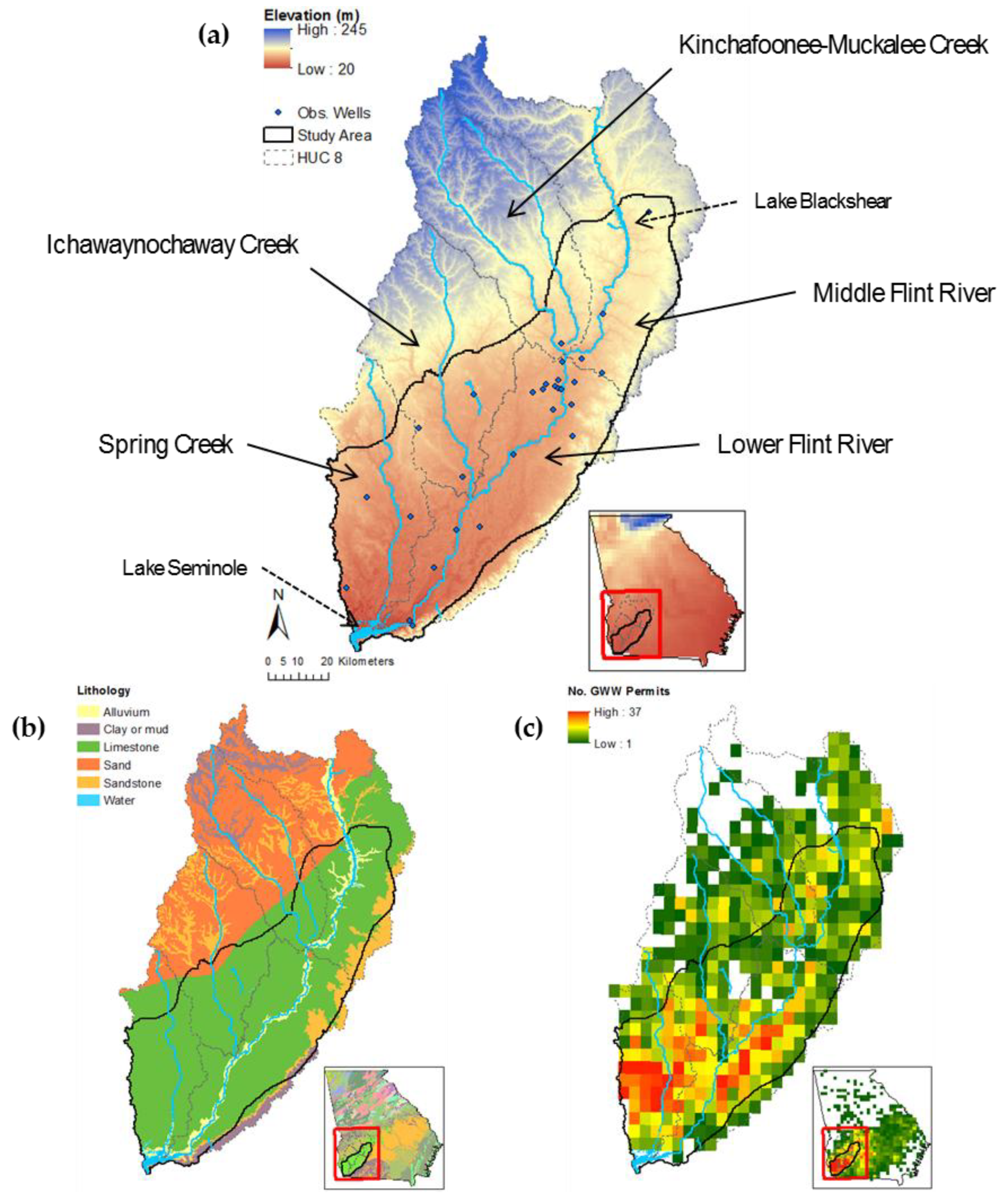
2.1. Study Area

The Flint River Basin (FRB) is a humid subtropical watershed located in the coastal plain of southwest Georgia. Agriculture is the primary industry in the basin, supporting a $5.8 billion economy [33]. The primary feature of the FRB is the Dougherty Plain, a low-lying area that is underlain by the regionally important upper Floridan aquifer (UFA) (Figure 1). Groundwater pumping in support of agriculture began in the mid-1970s with the introduction of center pivot irrigation systems. Today, 72% of irrigated acreage in the Lower FRB (LFRB) is supplied by groundwater [33]. Eighty percent of groundwater withdrawals in the basin come from the UFA, indicating that much of this use is concentrated in the Dougherty Plain underlain by the UFA (Figure 1) [34].
The Dougherty Plain was selected for this study due to observed spatial variability in groundwater flow patterns coupled with a strong seasonal drawdown signal and a large number (29) of USGS observation wells in the region (Figure 1). Dissolution of the Ocala Limestone that makes up the UFA has created a karstic aquifer system with a spatially heterogeneous transmissivity range that spans several orders-of-magnitude [35]. Field investigations indicate that in general, the conduit network of this karstic system is more well developed south and east of the Flint River; diffusive flow patterns tend to be more prevalent to the north and west [36]. Thickness of the UFA ranges from zero at its up-dip limit in the northwest to over 90 m at the southeastern margin of basin [37]. Close proximity of the UFA to the land surface within the Dougherty Plain makes it one of the primary recharge zones supplying the aquifer system (Figure 1). Previous work has also established the existence of strong yet spatially heterogeneous hydrologic connectivity between the UFA and streams within the FRB [38]. Observations of baseflow declines in streams across the FRB have been linked to substantial groundwater pumping for irrigation during the summer months [33,39]. Baseflow declines are seasonal, as winter recharge typically replenishes both surface water and groundwater systems [34].

2.2. Input Datasets and Pre-Processing

Eight hydrologic, climatic, and geologic predictor variables are used as inputs to the BRT model (Table 1). These parameters were chosen due to their impact on groundwater storage changes and previous sensitivity in other GRACE downscaling studies [28,31]. Where possible, raster datasets for each predictor were obtained for April 2002–December 2016, resampled or disaggregated to the target 0.05° (5 km) spatial resolution, and cropped to the study area extent. Variables not available in a gridded data product were converted to raster form.
Land surface temperature (LST) data was acquired from the Moderate Resolution Imaging Spectroradiometer (MODIS) MOD11C3 product with a 0.05° spatial resolution. No further processing was required because this already matched the target resolution. Normalized difference vegetation index (NDVI) data were obtained from the MODIS MOD13A3 product with 0.011° resolution and resampled to match the target resolution. An ensemble TWSA product was calculated by taking the mean of the University of Texas at Austin, Center for Space Research (CSR), the German Research Center for Geosciences (GFZ), and the Jet Propulsion Laboratories (JPL) RL-05 level-3 spherical harmonic solutions at 1° spatial resolution. Prior to the calculation of an ensemble mean, each product was scaled by the relevant scaling factor to correct for any signal loss that occurred during data processing [20].
Parameter-elevation Regressions on Independent Slope Model (PRISM) AN81m outputs provided precipitation data at 4-km resolution and were resampled to the target resolution. Two-meter soil moisture estimates were obtained from the Noah LSM NLDAS_NOAH0125_M product at 0.125° and disaggregated to the target resolution.
Discharge anomalies were derived from the average monthly discharge of the most downstream USGS stream gage in each HUC-8 sub-basin within the study area, preventing sub basins with larger streams from skewing the relationship fitted during model training. Anomalies were calculated relative to the mean monthly discharge at each gage from 2004–2009. Calculated anomalies for each month were then assigned to the entire sub-basin and converted to raster form. Lithology inputs were created by rasterizing a geologic map of the area and treated as a categorical, rather than a continuous, dataset in model training and prediction. Transmissivity of the UFA was estimated by using ordinary kriging to interpolate a transmissivity surface across the study area. Point transmissivity measurements from pump tests at 250 testing wells across the UFA used for interpolation came from USGS data release SIM 3204 [40].
Monthly GWLA at 29 USGS observation wells in the study area were used as the predictand in model training (Figure 1). GWLA was derived by converting mean monthly depth to water measurements to groundwater level measurements. Anomalies were then calculated using the mean monthly groundwater level from 2004–2009. Table 1 provides a summary of each input dataset and the processing steps taken.
Once all inputs were processed into monthly rasters with identical extents and the target 5-km spatial resolution, the predictor variables were associated with GWLA observations based on year, month, and observation well location within the input variable grid. For wells located near the edge of a grid cell, the distance-weighted average method developed by Seyoum et al. (2019) was applied to provide an estimate of predictor values based on the four cells closest to the well rather than simply the value of one grid cell [31].

2.3. Downscaling Method

Spatial downscaling of GRACE TWSA data was performed using a boosted regression tree (BRT) machine learning algorithm [41] applied to each cell in a prediction grid covering the study area. The BRT algorithm was selected because (1) unlike other machine learning methods, no prior data transformation of unit conversion is needed; (2) multiple predictor types (i.e., continuous and categorical) may be used as inputs; (3) the algorithm is unaffected by outliers and missing data within each observation/case; and (4) BRT is good at identifying and avoiding unimportant predictors based on the training data [42,43].
While BRT models are commonly used by ecologists for species distribution modeling [44,45], relatively few studies have used them for hydrologic mapping. Notable uses include the classification and prediction of soil properties [46,47] as well as the potential for groundwater resource development within specific watersheds [48,49]. In one of the more novel applications, Nolan et al. (2015) successfully used a BRT model to predict nitrate concentrations in groundwater within the Central Valley of California [50]. Some studies evaluated several different machine learning methods and found that BRT performed as well or better than other common algorithms [48,50,51,52].

2.4. BRT Training

Regression trees are a machine learning algorithm that utilizes recursive binary splits in an input dataset to determine where a given case falls within the prediction space (Figure 2), and are a form of the more general decision tree algorithm. Each split point—or node—on a tree is based on some value of a single predictor variable from the input dataset. For a given case at a node, if that case’s relevant variable is greater than or equal to some value the case is sent off to one node; if the variable is less than that value, the case is referred to another. This pattern is repeated until a stopping point is reached and the final prediction is made (Figure 2).
Training a single tree to be a so-called ‘strong learner’ may lead to overfitting and lack of model generalization. This may be prevented by using technique called gradient boosting to simultaneously improve model performance and limit overfitting. Rather than train a single strong learner, boosting algorithms use a linear combination of many weak learners to create an ensemble model [53]. As the number of individual trees in the ensemble grows, each new tree is fit to improve predictions for those cases that the current n-tree ensemble performs poorly on. This focused training improves the overall model fit to testing data [54].
Model optimization and training were performed using the “gbm” [55] and “dismo” [56] libraries within the R statistical programming language [57]. The optimal number of trees comprising the final BRT model was determined using 10-fold cross validation with tree complexity set to 10 and a learning, or shrinkage, rate of 0.005. Of the 29 observation wells within the study area with data available for at least half the study period, 20 were selected as training wells while the remaining 9 were withheld from the training phase to be used for model testing. It is also important to note that a monotonic response to the broad GRACE TWSA signal was assumed during model training.
Performance was dependent on which wells were selected for inclusion in the training dataset. Thus, the optimal distribution of training and testing wells was determined by training many models with randomly selected training wells. The ‘best’ distribution was selected by finding the training well set that led to the highest Nash–Sutcliffe Efficiency (NSE) value for predictions made on the corresponding testing well set. Once finalized, the BRT model was used to predict GWLA at each cell within the prediction grid to create monthly GWLA maps for April 2002–December 2016.

3. Results

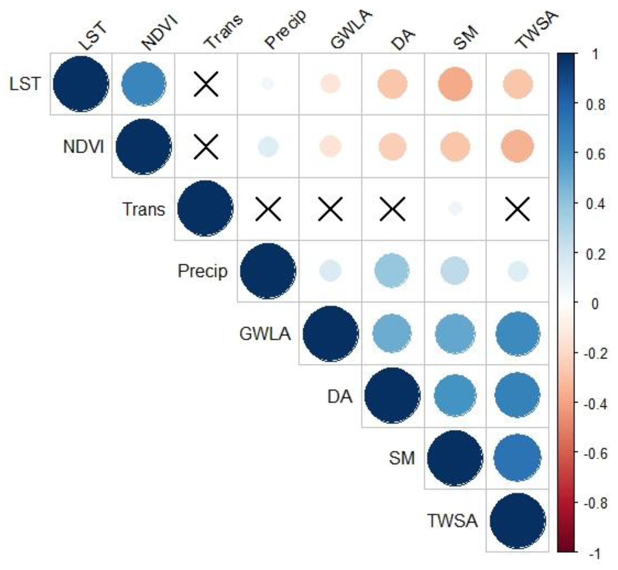
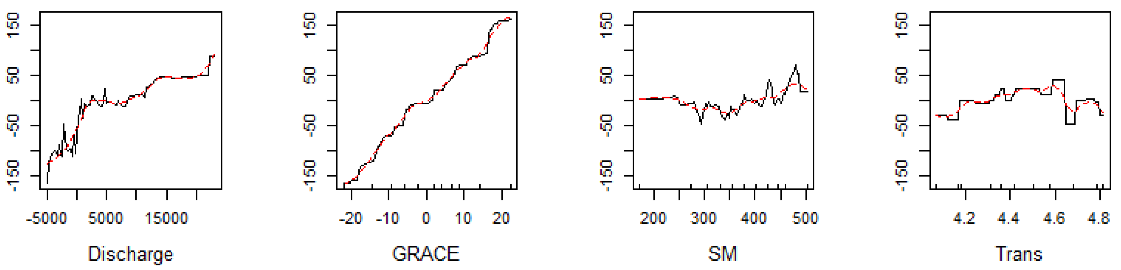
3.1. Data Correlations

Correlation tests between predictor variables and GWLA were performed prior to BRT training to identify interactions between the variables and determine which selected predictors showed the strongest correlation to GWLA in the study area (Figure 3). This served as an independent check on whether the relative importance of each predictor in the final trained BRT model is consistent with correlations observed in the dataset. Additionally, this provides a secondary benefit of looking for other interactions between predictor variables. All tests were performed using Pearson’s correlation coefficient and were significant if p < 0.05 and a critical value of 0.31. Lithology was not included in the correlation matrix, as it was treated as a categorical variable.
In decreasing order, GRACE TWSA, soil moisture, discharge anomaly, and monthly precipitation showed the strongest positive correlation with GWLA (Figure 3). This is to be expected, as TWSA and discharge anomaly control groundwater levels in a productive aquifer with strong hydrologic connectivity to the stream network [38]. Soil moisture is a more spatially heterogeneous indicator of how much water may actually be recharging the UFA. The negative correlation with LST and NDVI coupled with the positive GWLA correlation suggests that soil moisture influence on GWLA is due to recharge in the winter months rather than irrigation during the summer months. Weaker correlation between monthly precipitation in the cell overlaying a given well and GWLA may be due to a time lag in aquifer response to precipitation or a possible stronger dependence on precipitation in other cells overlaying this karstic aquifer [28].
LST and NDVI at each well showed a negative correlation with GWLA. This indicates the seasonality of the GWLA signal, as LST and NDVI are highest during the summer growing season. On the other hand, GWLA is highest during the winter season when most aquifer recharge occurs [34].
Transmissivity was the only selected predictor variable that did not show a statistically significant correlation with GWLA (R = 0.02, p = 0.31). Lack of temporal variation in the transmissivity input means that the transmissivity value at a given well is associated with the entire range of observed GWLAs at of that well. Thus, a correlation between the two cannot identify a unique relationship between transmissivity and GWLA. Transmissivity was still included as a predictor variable despite this artifact due its known importance to aquifer yield and groundwater flow patterns, especially in a karst basin.

3.2. Model Performance

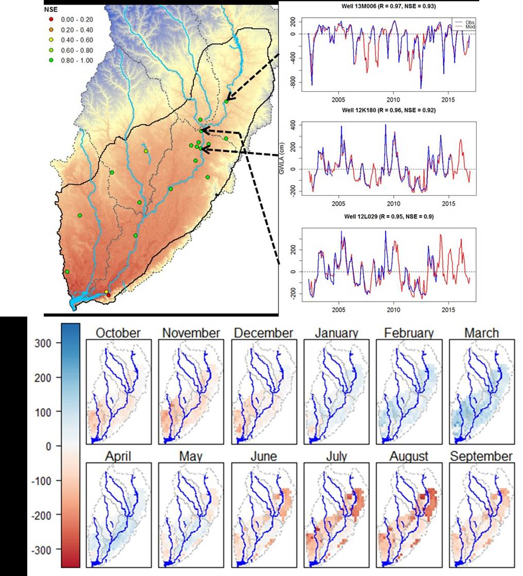
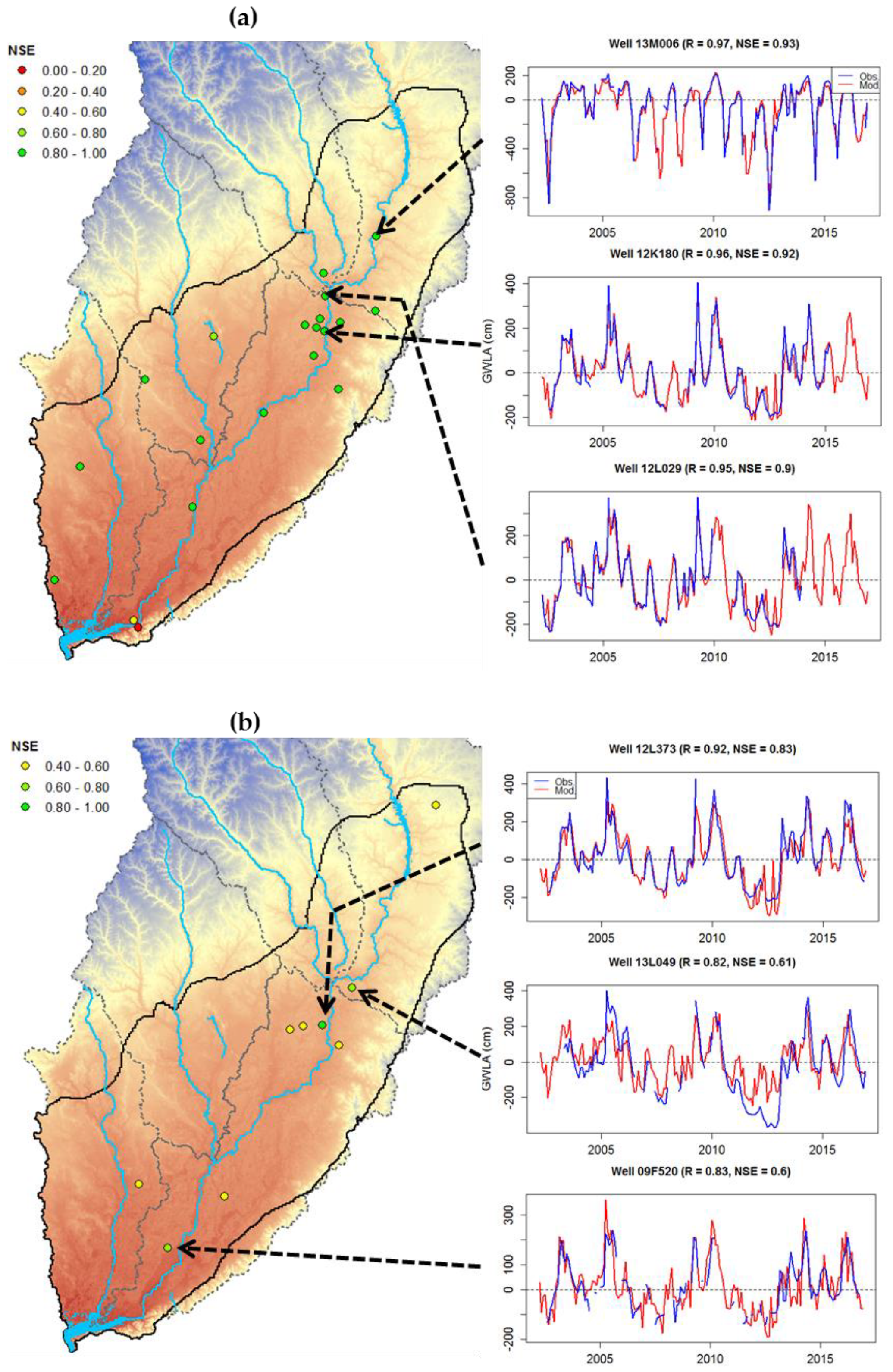
3.2.1. Overall Performance

Figure 4 shows scatter plots indicating the performance of the final BRT model trained using the optimal distribution of training and testing wells. During model training, the BRT algorithm was able to reach a solution that predicts GWLA based on the predictor variables with a high degree of accuracy (R = 0.97, NSE = 0.94). This confirms that the model is able to map a given set of input predictors to the predictand, despite the presence of complex interactions between them. Model performance in the testing phase indicates that the final trained BRT model adequately predicts GWLA at observation wells in the study area, with performance metrics falling within established ranges for satisfactory model performance (R = 0.79, NSE = 0.61, NRMSE = 0.62) [58]. Visual examination of the scatter plot for the testing phase indicates that model predictions have the highest error for predictions of negative GWLAs, over-predicting, and under-predicting in equal parts (Figure 4).

3.2.2. Individual Well Performance

The optimal distribution of training and testing wells as identified by highest testing phase NSE is shown in Figure 5. Training wells (Figure 5a) and testing wells (Figure 5b) are approximately evenly distributed throughout the study area given the original set of observation wells with monthly data for at least half of the GRACE period of record. All individual wells in the training phase had NSE > 0.80 regardless of location. The exceptions in the training phase are wells 10K005 (R = 0.84, NSE = 0.69), 08E039 (R = 0.80, NSE = 0.50), and 08E038 (R = 0.68, NSE = 0.06). Well 10K005 is located in a wetland area and likely is governed by a different groundwater regime than the rest of the karstic UFA, while wells 08E039 and 08E038 are located along the shores of Lake Seminole reservoir at the southernmost extent of the study area. Reservoir levels and dam release schedules play a stronger role in controlling groundwater levels in these wells. NSE in testing phase wells ranges from 0.41 to 0.83, with the best fits occurring at wells in the central region of the study area with the highest concentration of observation wells (Figure 5b).
Plots beside Figure 5 compare observed and modeled time series for the top three simulated wells from each set along with their locations within the study area. All wells shown appear to have the most error relative to the rest of their respective time series from 2010–2013, a period of severe regional drought. These more pronounced errors may be due to other variables beginning to exert more influence on groundwater levels during drought periods that were not included as predictor variables or that the surface water–groundwater exchange is non-existent during drought, causing it to miss important drivers and shows a potential shortcoming in the model during severe drought periods. Despite this, time series for the training well set indicate that a properly parameterized BRT or other machine learning model could be effective for gap filling of missing well data if those wells are used for model training (Figure 5).

3.3. Map Products

GWLA maps were produced for each month in the study period with data from all three GRACE processing centers for calculation of an ensemble mean. Output of the spatial prediction after model training and testing on individual wells is a 5-km raster covering the study area within the LFRB. Sub-basins that were missing stream gage data for calculation of a discharge anomaly in a given month were not modeled for that month.
Figure 6 shows a set of example monthly GWLA maps for water year 2007. These indicate lower groundwater levels across the study area at the beginning of the water year, with the system recovering to conditions either at or slightly above the 2004–2009 GRACE mean (Level 3 GRACE product anomalies are relative to this baseline from the NASA MEaSUREs program) from December 2006–January 2007. Some negative anomalies begin to occur in the beginning of the annual groundwater pumping season (April 2007), which peak in July–September 2007. September spatial predictions begin to show some recovery in the aquifer, however.
The strongest signals are found in the up-dip northwestern and northeastern portions of the study area. In particular, the Spring Creek sub-basin has both one of strongest signals and the most intra-sub-basin variability, with the highest GWLA amplitudes occurring in the northern portion of the sub-basin. This is also the area with the highest density of groundwater withdrawal permits in the entire study area (Figure 1c). In the Middle Flint River sub-basin, the small region of slightly positive GWLA corresponds to the location of the Lake Blackshear reservoir. Spatial predictions correctly identify this reservoir from soil moisture, LST, and NDVI despite the lack of any explicit indication of reservoir locations within the predictor variables. Some of the strongest negative signals are also seen within this sub-basin. Along the southeastern margin of the study area lies a thin sliver of negative GWLA during the growing season, despite the generally positive GWLAs observed in the rest of the basin. This is an upland region marking the beginning of the Pelham Escarpment and the confinement of the UFA (Figure 1a). Although there are no observation wells here, predictor variable distributions in this region are similar to those found at the poorly modeled observation well 08E038 (Figure 5a and Figure 6). Thus, predicted GWLA are likely not representative of groundwater conditions.

3.4. Model Behavior

3.4.1. Relative Influence

One advantage of using a BRT algorithm is the relative transparency of the final model and ease with which the influence of the predictor variables may be evaluated (Figure 7). The relative influence of each predictor is quantified by counting how often a given variable is used for splitting. Each count is weighted by the model improvement it accounts for and is averaged over all trees in the ensemble model. Finally, this sum of weighted counts for each variable is converted to a percentage [41,59].
Discharge anomaly, rather than GRACE TWSA, was the most important predictor variable identified by the model with TWSA the second most important by a wide margin. This is consistent with prior determinations of the significance of groundwater–surface water interactions relative to groundwater conditions in the study area. Additionally, the importance of discharge anomalies explains the occasional sharp changes in predicted GWLA across sub-basin boundaries, as discharge anomaly was discretized at the sub-basin scale. Soil moisture and transmissivity are nearly identical in terms of relative influence within the model. As discussed earlier, soil moisture may serve as a proxy for potential recharge to the UFA while transmissivity is the only input that provides information on subsurface flow patterns.
Relative influence of predictor variables within the model is mostly consistent with the correlations to GWLA observed in Figure 3. Although the ordering is slightly different, the three variables with the highest correlation to GWLA are also the three variables with the most influence in the BRT model trained to predict GWLA. Notably, transmissivity is nearly as influential in predicting GWLA as soil moisture despite the lack of a statistically significant correlation in Figure 3. The minimal influence of lithology as a predictor is due to the nearly homogenous presence of limestone within the study area (Figure 1b).

3.4.2. Partial Dependence

Partial dependence plots were used to further investigate the role of the four most influential predictors in the final BRT model (Figure 8). Such plots serve as a form of sensitivity analysis for machine learning models by determining the marginal effect a given predictor has on the output of a trained model [41]. As expected, discharge anomaly and GRACE TWSA exert a strong influence on predicted GWLA. Negative discharge anomalies have a stronger effect than positive anomalies, quickly decreasing GWLA and pulling it into the negative range. The relationship between GRACE TWSA and GWLA is approximately linear partially due to the forced monotonic relationship during model training, although it is far from 1:1.
Soil moisture and transmissivity show less definite effects on model predictions. Low to mid-range soil moisture conditions in the growing season generate negative GWLA predictions, while higher winter soil moisture conditions lead to positive GWLA. Transmissivity creates negative predictions on either end of the domain with a positive peak in the middle. Given that the transmissivity inputs were constant, this is more reflective of observation well positioning rather than a true relationship; however, it is notable that at a certain threshold GWLA predictions drop sharply into the negative range.

3.4.3. Role of Soft Data in Predictions

GRACE TWSA and discharge anomaly may both be considered as soft data inputs to the BRT model in this study [60]. Soft data inputs include areal estimates and large scale information that integrates the effects of several processes (e.g., regional ET estimates, average annual runoff coefficients) [60]. Given the unique characteristics of this karstic basin, there is a possibility that both inputs provide similar water storage information to the model and may be redundant. Although GRACE TWSA shows a stronger correlation with GWLA than discharge anomaly in the training and testing datasets, the greater influence of discharge anomaly as a predictor in the model calls into question the predictive value added by including GRACE as a redundant input.
Two additional BRT models were trained on the same wells as the original model to evaluate whether a model trained on a given set of wells would perform better by only including one of these soft datasets. One of these models dropped GRACE TWSA as an input, while the other dropped discharge anomaly. Relative influence plots of each model show that in the respective soft data input in each model remained the most important predictor (Figure 9). Model performance on the testing data (as indicated by NSE) decreased by 23% and 18%, respectively. Results indicate that GRACE does indeed add predictive value to the model despite providing similar information to discharge anomalies. Furthermore, the use of both inputs still provides a significant improvement in performance. This indicates that the soft information provided to the model by both datasets has a synergistic effect in the study area by capturing large-scale behaviors of the strongly related systems they represent.

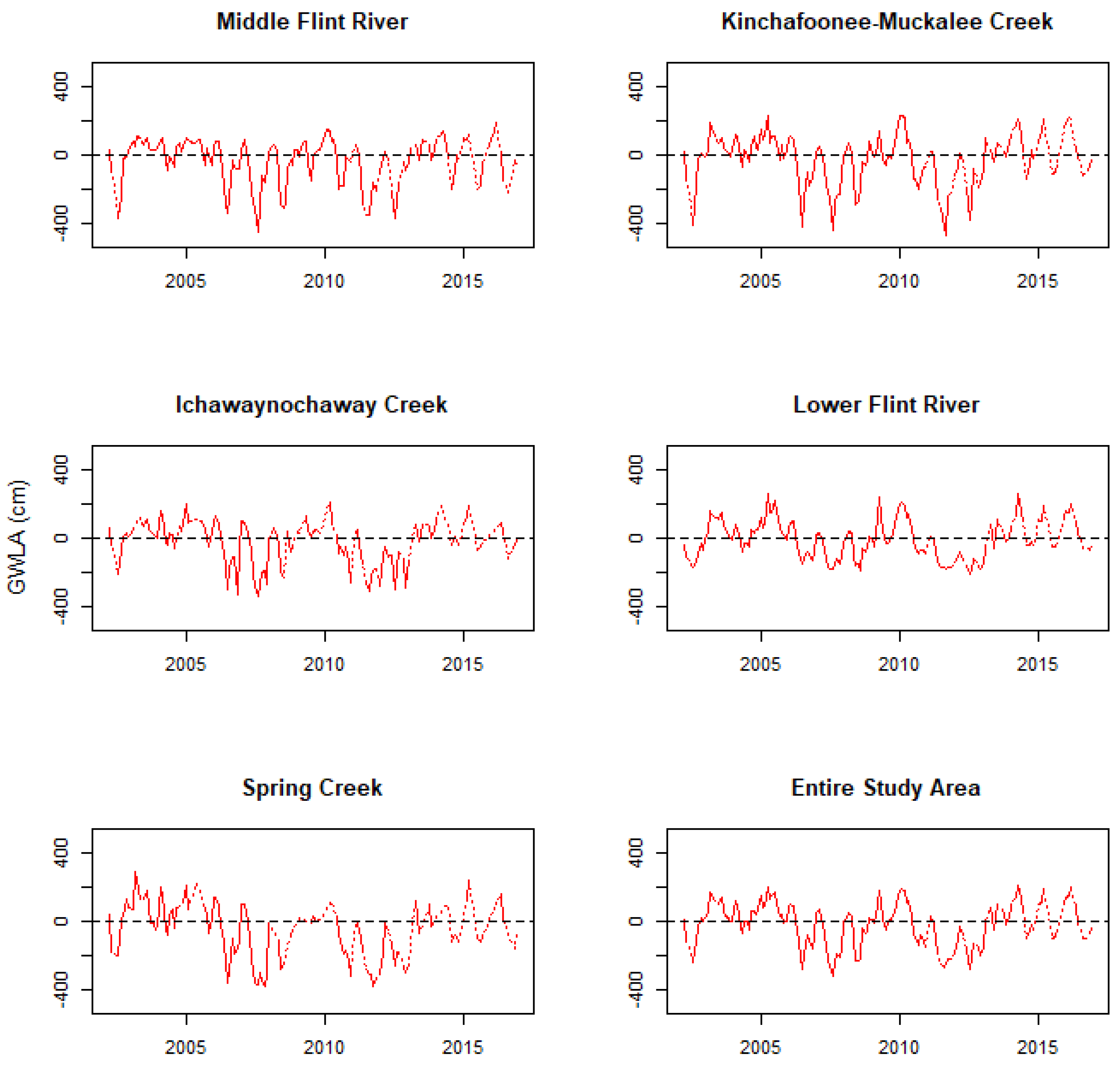
3.5. Spatial Patterns of Groundwater Drawdown

3.5.1. Overall Patterns

While investigating the interactions present in the trained model illuminates drivers of GWLA within the study area, aggregating spatial predictions from the model allows for an investigation of long-term and intra-annual patterns of GWLA that are informed both by in situ data and GRACE observations (Figure 10). Figure 10a shows the mean predicted GWLA for each grid cell across the entire study period. Results show that groundwater levels generally remain stable in much of the study area. The Lower Flint River is the only sub-basin that shows substantial areas of positive mean GWLA, with neutral and negative values spread throughout. Despite the prevalence of positive values, most are < +50 cm. Ichawaynochaway Creek, Kinchafoonee-Muckalee Creek, and Middle Flint River sub-basins have slightly negative mean GWLA predictions, again rarely > -50 cm in magnitude. Grid cells overlying Lake Blackshear have almost no mean anomaly, again pointing to consistent identification of this feature by the model. The relatively lighter cells on the eastern margin of Ichawaynochaway Creek sub-basin correspond to extensive wetlands, shifting more toward negative anomalies in the central and western regions of the sub-basin. Spring Creek sub-basin has the highest magnitude negative mean GWLA predictions in the study area. In particular, one group of cells in the south-central region shows anomalously high negative GWLA predictions approaching -100 cm. The northwestern portion of the study area near the up-dip extent of the UFA also shows consistently high GWLA predictions, along with isolated cells along the eastern margin of the sub-basin.
Variability of model predictions was quantified by calculating the interquartile range (IQR) of GWLA predictions in each cell (Figure 10b). This allows for determining the typical amplitude of predictions for each cell without being driven by outliers in the data. Much of the study area shows a typical fluctuation of < 300 cm. Regions of the study area with the lowest IQR generally correspond to water bodies (i.e., Lake Seminole and Lake Blackshear) and forested or wetland areas. The most prominent feature of Figure 10b is the presence of IQR values > 300 cm in the northern half of the Spring Creek sub-basin. Rather than corresponding to the isolated central hotspot of large negative mean anomalies seen in Figure 10a, which have and average to below average IQR, this area corresponds to the northern cells with varying magnitudes of negative GWLA. Notably, the highest IQR values occur in the cells with the largest negative mean GWLA.

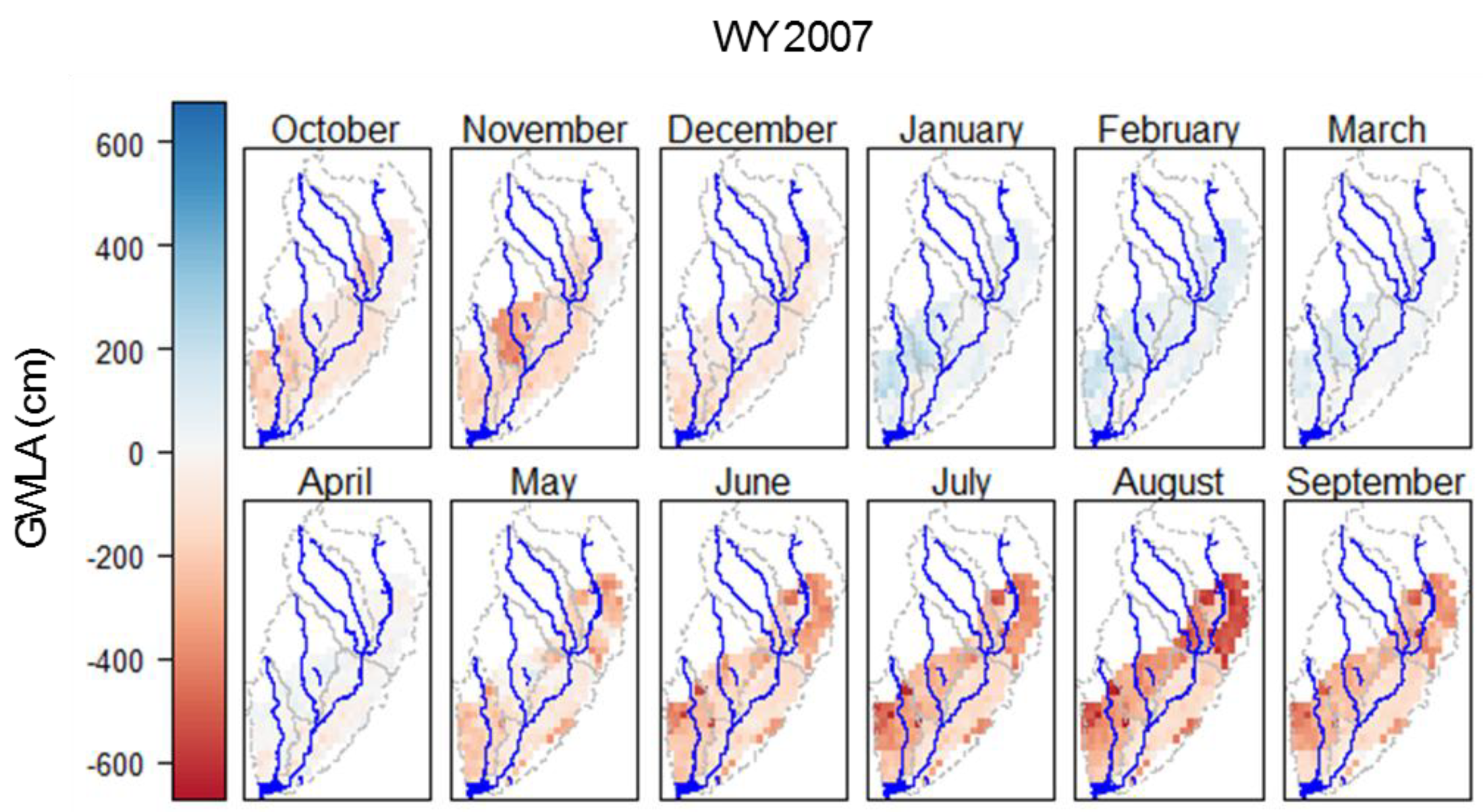
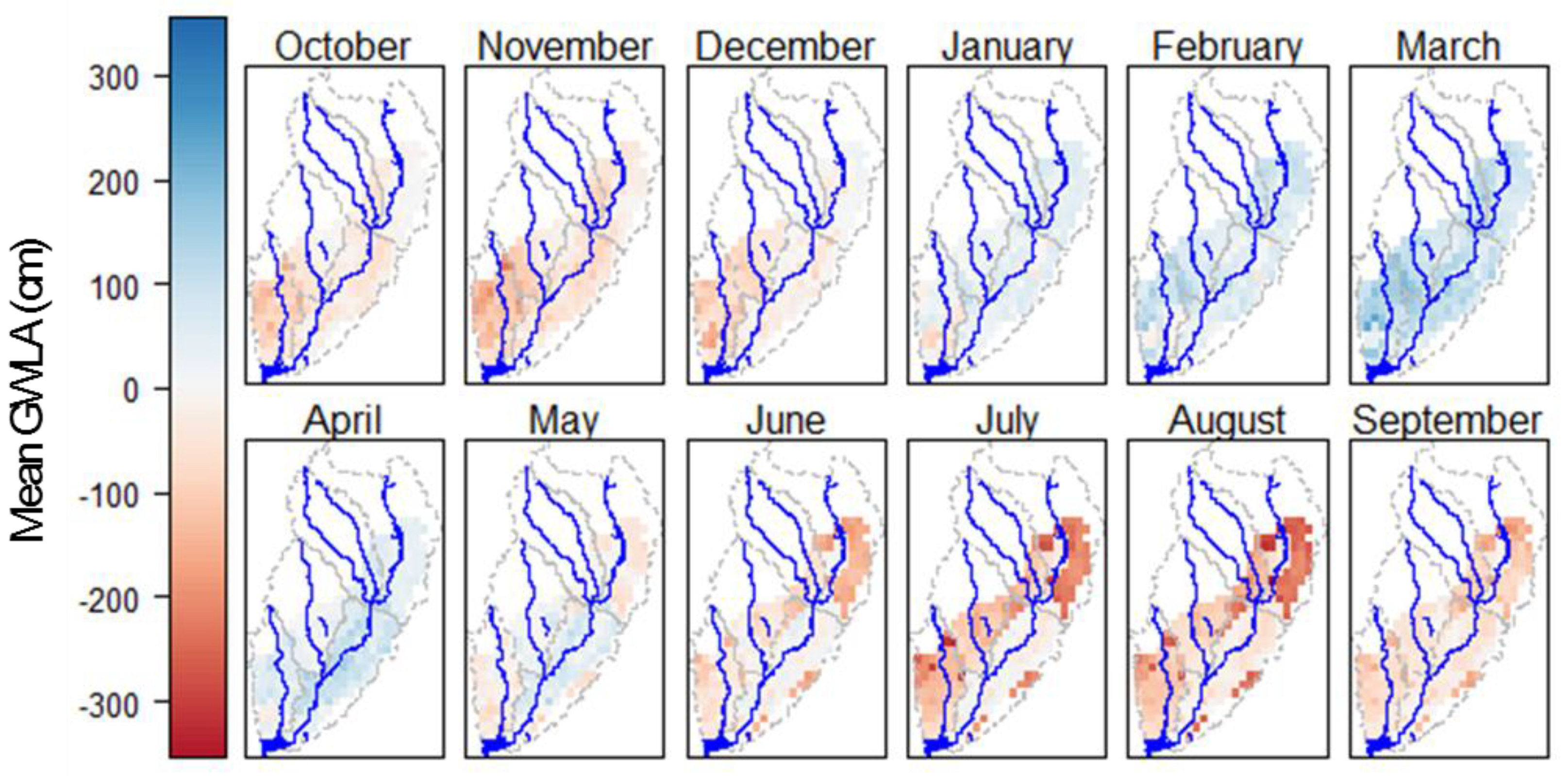
3.5.2. Monthly Patterns

Calculation of monthly mean GWLA predictions allows for an assessment of seasonal oscillations within the study period, revealing a cyclical pattern of aquifer drawdown and recharge (Figure 11). Across the study area negative GWLA reaches a maximum in July and August, particularly in the Middle Flint River and Kinchafoonee–Muckalee Creek sub-basins. Groundwater levels begin to recover September–October, with full recovery occurring by January. Most recharge occurs from January–March, when groundwater levels peak across the study area before levels drop from April–August. While negative anomalies are highest in the Middle Flint River sub-basin, positive anomalies are highest in the Spring Creek sub-basin with the exception of single anomalous cells seen in Figure 10. In addition, the hotspot of negative mean GWLA in the central Spring Creek sub-basin reaches anomalously low positive values, taking longer to recharge than the surrounding areas and beginning to deplete earlier.

4. Discussion

4.1. Efficacy of the BRT Downscaling Approach

Performance metrics during the model training and testing phases indicate that the model is successful in creating GWLA predictions for observation wells (Figure 4 and Figure 5). This points to the success of the model as a means to downscale GRACE TWSA observations by using it as a “soft data” input for spatial predictions of GWLA [60]. Although discharge anomalies proved to be more important than GRACE data for model predictions, GRACE is still the second most important predictor. In early model runs that did not include discharge anomaly as an input, GRACE data were generally always the most influential variable in trained models. The diminished importance of GRACE is due to the unusually high degree of hydrologic connectivity between groundwater and surface water systems in the basin, which mean stream discharge anomalies serve as strong indicators of overall groundwater conditions. Future work should consider applying a similar approach in aquifer systems that are disconnected from the overlying surface water system. These more pronounced errors in Figure 5 might be due to other variables beginning to exert more influence on groundwater levels during drought periods that were not included as predictor variables or that the surface water– groundwater exchange is non-existent during drought causing it to miss important drivers and shows a potential shortcoming in the model during severe drought periods. Houborg et al., (2012) assimilated GRACE observations into a CLM to improve drought prediction, which demonstrates the utility of GRACE in drought research. Nevertheless, time series for the training well set indicate that a properly parameterized BRT or other machine learning model could be effective for gap filling of missing well data if those wells are used for model training (Figure 5).
Although more investigation is needed, properly executed machine learning based downscaling techniques have several potential benefits provided appropriate predictors and validation is applied. (1) Investigations may be performed remotely using publically available datasets and open access software. (2) The ability of machine learning techniques to identify complex relationships in the input dataset could provide new insights into the interplay between predictors and how they interact to make model predictions. (3) The final BRT model proved to be effective for gap-filling of missing groundwater level data at observation wells included in the training dataset (Figure 5), a by-product that has been more fully studied by others [26]. It is important that models are trained on wells to be gap-filled though, as predictions for testing wells tend to have a higher error associated with them.

4.2. Model Insights

Model predictions generally confirm conclusions by previous researchers [34,36] that the portion of the UFA within the study area is not experiencing long-term groundwater depletion (Figure 10, Figure 11 and Figure 12). While most cells show non-zero mean GWLA predictions, these deviations are small in magnitude. Additionally, relationships in the assembled dataset identified by the model confirm the strong relationship between the groundwater and surface water systems in the FRB (Figure 8) [38,39]. The partial dependence plot for discharge anomaly shown in Figure 8 indicates some asymmetry in model predictions during high and low flow conditions. Predicted GWLAs are less stable for negative values of discharge anomaly than for positive values; this may be due to changes in the groundwater flow regime during low flow conditions in the surface water system or simply seasonal influences.
Notable exceptions to the stability of the groundwater system during the study period include the Middle Flint River and Spring Creek sub-basins. Hicks et al. (1987) determined that the eastern and northeastern portions of the Middle and Lower Flint River sub-basins, respectively, are underlain by a higher density of dissolution features in the Ocala Formation [36]. However, the region of positive GWLA predictions across the Flint River in the northern Lower Flint River sub-basin was found to exhibit diffuse flow properties. The area of negative predictions west of that and extending into the Ichawaynochaway Creek sub-basin is possibly underlain by caverns in the UFA [61].
Strong signals seen in the Spring Creek sub-basin are supported by other observations, however. This sub-basin is the most heavily allocated in Georgia in terms of groundwater resources, with documented decreases in summer baseflow and transition from a perennial to an ephemeral stream since the beginning of widespread groundwater pumping for irrigation in the mid-1970s [39]. The hydrograph from a USGS stream gage near the central hotspot of negative mean GWLA confirms that stretch Spring Creek periodically ran dry throughout the study period. Additionally, the highest groundwater withdrawal permit density in the study area almost completely overlaps with this area (Figure 1c). Groundwater flow is north to south, potentially explaining the slight southern shift of the hotspot and suggesting that groundwater levels in the UFA are more sensitive to groundwater pumping in this area. However, further investigation would be required to confirm this.

4.3. Potential Issues and General Applicability

Although the downscaling method used here shows promise, there are key points that should be stated for future use. First, the use of this method is limited by the number of observation wells with continuous data over long periods. This also means that is difficult to set aside sufficient wells for the creation of independent GWLA surfaces for the evaluation of spatial predictions. Additionally, model predictions are only as good as the dataset the model is trained on. It is possible the important predictor datasets may not be available in some areas. In the absence of critical datasets, the model may not be general enough and provide too much importance to irrelevant predictors in pursuit of satisfying the objective function. Finally, this method assumes that GWLA in a particular cell is a function of co-located predictor values. While the spatial autocorrelation of predictor values and the interpolation of a transmissivity surface for this study means that the model is partially informed by surrounding grid cells, the conduit network of the karstic UFA likely plays a strong role in groundwater behavior in the eastern portion of the study area [36]. This is a critical component of the flow regime in karstic groundwater systems, and one that previous researchers using machine learning models to predict point groundwater levels in karstic systems have ignored [62]. Ideally, future studies would include a stronger accounting of parameters controlling subsurface flow in this and other heterogeneous systems.

5. Conclusions

In the face of groundwater depletion issues affecting dependent populations worldwide, TWSA observations from the GRACE satellite system have become a powerful tool for assessing the degree and spatial pattern of groundwater change. However, the coarse spatial resolution of these observations has plagued efforts to understand more local changes in groundwater. More studies are beginning to use powerful machine learning algorithms to downscale GRACE observations, but relatively few have generated the type of spatially downscaled gridded products that are most useful to resource managers [30,31]. This study successfully trained a BRT model to downscale GRACE TWSA observations to 5 km GWLA predictions in the heavily allocated karstic UFA using a suite of other hydrologic and geologic datasets. Monthly spatial predictions of GWLA output by the model confirmed previous conclusions that, despite widespread drawdowns during the summer months, groundwater levels are mostly stable in the long term. Model outputs also identified a part of the study area in the Spring Creek sub-basin that consistently experiences anomalously strong drawdowns. Although the high density of groundwater withdrawal permits region suggests this may be due to groundwater pumping, more work would be required to test this hypothesis. While machine learning based GRACE downscaling approaches are easily applicable to other regions, users should ensure availability of proper datasets for model training and validation. Future studies in karstic systems should pay particular attention to better inclusion of conduit networks when selecting predictor variables.

Author Contributions

A.M.M. was responsible for project administration, conceptualization of the project, interpreting the results, and manuscript preparation and writing. M.B.T. helped carry out the methodology, provided R software processing, analysis, and writing of the manuscript. W.M.S. aided in the conceptualization of the project, designing the methodology, interpreting results, and reviewing the manuscript. T.C.R. was responsible for the formal analysis, project oversight, manuscript review, and project conceptualization related to the Flint River and Upper Floridan Aquifer.

Funding

This research was funded by the University of Georgia’s Watts-Wheeler Fund. Publication costs were supported by the Warnell School of Forestry & Natural Resources and the Department of Geology at the University of Georgia.

Acknowledgments

The authors wish to thank Dongjae Kwon for sharing his technical knowledge and assisting with the implementation of this work.

Conflicts of Interest

The authors declare no conflict of interest.

References

  1. UNESCO. Water Ethics and Water Resource Management; UNESCO: Bangkok, Thailand, 2011; ISBN 9789292233587. [Google Scholar]
  2. Wada, Y.; Van Beek, L.P.H.; Van Kempen, C.M.; Reckman, J.W.T.M.; Vasak, S.; Bierkens, M.F.P. Global depletion of groundwater resources. Geophys. Res. Lett. 2010, 37, 1–5. [Google Scholar] [CrossRef]
  3. Frimpong, Y.; Oluwoye, J.; Crawford, L. Causes of delay and cost overruns in construction of groundwater projects in a developing countries; Ghana as a case study. Int. J. Proj. Manag. 2003, 21, 321–326. [Google Scholar] [CrossRef]
  4. Mogheir, Y.; De Lima, J.L.M.P.; Singh, V.P. Assessment of informativeness of groundwater monitoring in developing regions (Gaza Strip Case Study). Water Resour. Manag. 2005, 19, 737–757. [Google Scholar] [CrossRef]
  5. Milewski, A.; El Kadiri, R.; Durham, M. Assessment and intercomparison of TMPA satellite precipitation products in varying climatic and topographic regimes in morocco. Remote Sens. 2015, 7, 5697–5717. [Google Scholar] [CrossRef]
  6. Milewski, A.; Sultan, M.; Yan, E.; Becker, R.; Abdeldayem, A.W.; Gelil, K.A. Remote sensing solutions for estimating runoff and recharge in arid environments. J. Hydrol. 2009, 373, 1–14. [Google Scholar] [CrossRef]
  7. Bierkens, M.F.P. Global hydrology 2015: State, trends, and directions. Water Resour. Res. 2016, 51, 4923–4947. [Google Scholar] [CrossRef]
  8. Lettenmaier, D.P.; Alsdorf, D.; Dozier, J.; Huffman, G.J.; Pan, M.; Wood, E.F. Inroads of remote sensing into hydrologic science during the WRR era. Water Resour. Res. 2015, 51, 7309–7342. [Google Scholar] [CrossRef]
  9. Tapley, B.D.; Bettadpur, S.; Watkins, M. The gravity recovery and climate experiment: Mission overview and early results. Geophys. Res. Lett. 2004, 31. [Google Scholar] [CrossRef]
  10. Wahr, J.; Swenson, S.; Zlotnicki, V.; Velicogna, I. Time-variable gravity from GRACE: First results. Geophys. Res. Lett. 2004, 31, 20–23. [Google Scholar] [CrossRef]
  11. Yeh, P.J.F.; Swenson, S.C.; Famiglietti, J.S.; Rodell, M. Remote sensing of groundwater storage changes in Illinois using the Gravity Recovery and Climate Experiment (GRACE). Water Resour. Res. 2006, 42. [Google Scholar] [CrossRef]
  12. Rodell, M.; Velicogna, I.; Famiglietti, J.S. Satellite-based estimates of groundwater depletion in India. Curr. Sci. 2009, 460, 999–1003. [Google Scholar] [CrossRef] [PubMed]
  13. Famiglietti, J.S.; Lo, M.; Ho, S.L.; Bethune, J.; Anderson, K.J.; Syed, T.H.; Swenson, S.C.; De Linage, C.R.; Rodell, M. Satellites measure recent rates of groundwater depletion in California’s Central Valley. Geophys. Res. Lett. 2011, 38, 2–5. [Google Scholar] [CrossRef]
  14. Scanlon, B.R.; Faunt, C.C.; Longuevergne, L.; Reedy, R.C.; Alley, W.M.; McGuire, V.L.; McMahon, P.B. Groundwater depletion and sustainability of irrigation in the US High Plains and Central Valley. Proc. Natl. Acad. Sci. USA 2012, 109, 9320–9325. [Google Scholar] [CrossRef] [PubMed]
  15. Feng, W.; Zhong, M.; Lemoine, J.M.; Biancale, R.; Hsu, H.T.; Xia, J. Evaluation of groundwater depletion in North China using the Gravity Recovery and Climate Experiment (GRACE) data and ground-based measurements. Water Resour. Res. 2013, 49, 2110–2118. [Google Scholar] [CrossRef]
  16. Lezzaik, K.; Milewski, A. A quantitative assessment of groundwater resources in the middle east and north africa region. Hydrogeology 2018, 26, 251. [Google Scholar] [CrossRef]
  17. Sultan, M.; Metwally, S.; Milewski, A.; Becker, D.; Ahmed, M.; Sauck, W.; Soliman, F.; Sturchio, N.; Wagdy, A.; Becker, R.; et al. Modern recharge to fossil aquifers: Geochemical, geophysical, and modeling constraints. J. Hydrol. 2011, 403, 14–24. [Google Scholar] [CrossRef]
  18. Lezzaik, K.; Milewski, A.; Mullen, J. The groundwater risk index: Development and application in the Middle East and North Africa region. Sci. Total Environ. 2018, 628, 1149–1164. [Google Scholar] [CrossRef]
  19. Famiglietti, J.S.; Rodell, M. Environmental science. Water in the balance. Science 2013, 1300–1302. [Google Scholar] [CrossRef]
  20. Landerer, F.W.; Swenson, S.C. Accuracy of scaled GRACE terrestrial water storage estimates. Water Resour. Res. 2012, 48. [Google Scholar] [CrossRef]
  21. Swenson, S.; Wahr, J. Post-processing removal of correlated errors in GRACE data. Geophys. Res. Lett. 2006, 33, 1–4. [Google Scholar] [CrossRef]
  22. Fowler, H.J.; Blenkinsop, S.; Tebaldi, C. Linking climate change modelling to impacts studies: Recent advances in downscaling techniques for hydrological modelling. Int. J. Climatol. 2007, 4, 1547–1555. [Google Scholar] [CrossRef]
  23. Lo, M.H.; Famiglietti, J.S.; Yeh, P.J.F.; Syed, T.H. Improving parameter estimation and water table depth simulation in a land surface model using GRACE water storage and estimated base flow data. Water Resour. Res. 2010, 46, 1–15. [Google Scholar] [CrossRef]
  24. Sun, A.Y.; Green, R.; Swenson, S.; Rodell, M. Toward calibration of regional groundwater models using GRACE data. J. Hydrol. 2012, 422, 1–9. [Google Scholar] [CrossRef]
  25. Houborg, R.; Rodell, M.; Li, B.; Reichle, R.; Zaitchik, B.F. Drought indicators based on model-assimilated Gravity Recovery and Climate Experiment (GRACE) terrestrial water storage observations. Water Resour. Res. 2012, 48. [Google Scholar] [CrossRef]
  26. Sun, A.Y. Predicting groundwater level changes using GRACE data. Water Resour. Res. 2013, 49, 5900–5912. [Google Scholar] [CrossRef]
  27. Haykin, S. Neural Networks and Learning Machines, 3rd ed.; Prentice Hall: Lawrence, KS, USA, 2009. [Google Scholar]
  28. Seyoum, W.M.; Milewski, A.M. Improved methods for estimating local terrestrial water dynamics from GRACE in the Northern High Plains. Adv. Water Resour. 2017, 110, 279–290. [Google Scholar] [CrossRef]
  29. Gemitzi, A.; Lakshmi, V. Estimating groundwater abstractions at the aquifer scale using GRACE observations. Geosciences 2018, 8, 419. [Google Scholar] [CrossRef]
  30. Miro, M.E.; Famiglietti, J.S. Downscaling GRACE remote sensing datasets to high-resolution groundwater storage change maps of California’s Central Valley. Remote Sens. 2018, 10, 143. [Google Scholar] [CrossRef]
  31. Seyoum, W.M.; Kwon, D.; Milewski, A.M. Downscaling GRACE TWSA data into high-resolution groundwater level anomaly using machine learning-based models in the glacial aquifer system. Remote Sens. 2019, 11, 824. [Google Scholar] [CrossRef]
  32. Jacob, T.; Bayer, R.; Chery, J.; Le Moigne, N. Time-lapse microgravity surveys reveal water storage heterogeneity of a karst aquifer. J. Geophys. Res. Solid Earth 2010, 115, 1–18. [Google Scholar] [CrossRef]
  33. Couch, C.A.; McDowell, R.J. Flint River Basin Regional Water Development and Conservation Plan; Georgia Department of Natural Resources-Environmental Protection Division: Atlanta, GA, USA, 2006. [Google Scholar]
  34. Torak, L.J.; Painter, J. Geohydrology of the Lower Apalachicola–Chattahoochee–Flint River Basin, Southwestern Georgia, Northwestern Florida and Southeastern Alabama; USGS: Reston, VA, USA, 2006.
  35. Torak, L.J.; McDowell, R.J. Ground-Water Resources of the Lower Apalachicola-Chattahoochee-Flint River Basin in Parts of Alabama, Florida, and Georgia—Subarea 4 of the Apalachicola-Chattahoochee-Flint and Alabama-Coosa-Tallapoosa River Basins; National Park Service: Washington, DC, USA, 1996. [Google Scholar]
  36. Hicks, D.W.; Gill, H.E.; Longsworth, S.A. Hydrogeology, Chemical Quality, and Availability of Ground Water in the Upper Floridan Aquifer, Albany Area, Georgia; Water-Resources Investigations Report 87–4145; U.S. Geological Survey: Doraville, GA, USA, 1987; 31p.
  37. Torak, L.J. A MODular Finite-Element model (MODFE) for areal and axisymmetric ground-water-flow problems, part 1: Model description and user’s manual. In Techniques of Water-Resources Investigations; Book 6; US Geological Survey: Reston, VA, USA, 1993. [Google Scholar]
  38. Rugel, K.; Golladay, S.W.; Jackson, C.R.; Rasmussen, T.C. Delineating groundwater/surface water interaction in a karst watershed: Lower Flint River Basin, southwestern Georgia, USA. J. Hydrol. Reg. Stud. 2016, 5, 1–19. [Google Scholar] [CrossRef] [Green Version]
  39. Rugel, K.; Jackson, C.R.; Romeis, J.J.; Golladay, S.W.; Hicks, D.W.; Dowd, J.F. Effects of irrigation withdrawals on streamflows in a karst environment: Lower Flint River Basin, Georgia, USA. Hydrol. Process. 2012, 26, 523–534. [Google Scholar] [CrossRef]
  40. Kuniansky, E.L.; Bellino, J.C.; Dixon, J.F. Transmissivity of the Upper Floridan Aquifer in Florida and Parts of Georgia, South Carolina, and Alabama; US Geological Survey: Reston, VA, USA, 2012.
  41. Friedman, J.H. Greedy function approximation: A gradient boosting machine. Ann. Stat. 2001, 29, 1189–1232. [Google Scholar] [CrossRef]
  42. Elith, J.; Leathwick, J.R.; Hastie, T. A working guide to boosted regression trees. J. Anim. Ecol. 2008, 77, 802–813. [Google Scholar] [CrossRef] [PubMed]
  43. Breiman, L. Statistical modeling: The two cultures. Stat. Sci. 2001, 16, 199–231. [Google Scholar] [CrossRef]
  44. De’ath, G.; Fabricius, K.E. Classification and regression trees: A powerful yet simple technique for ecological data analysis. Ecology 2000, 81, 3178–3192. [Google Scholar] [CrossRef]
  45. Leathwick, J.R.; Elith, J.; Francis, M.P.; Hastie, T.; Taylor, P. Variation in demersal fish species richness in the oceans surrounding New Zealand: An analysis using boosted regression trees. Mar. Ecol. Prog. Ser. 2006, 321, 267–281. [Google Scholar] [CrossRef] [Green Version]
  46. Lemercier, B.; Lacoste, M.; Loum, M.; Walter, C. Extrapolation at regional scale of local soil knowledge using boosted classification trees: A two-step approach. Geoderma 2012, 171, 75–84. [Google Scholar] [CrossRef]
  47. Jorda, H.; Bechtold, M.; Jarvis, N.; Koestel, J. Using boosted regression trees to explore key factors controlling saturated and near-saturated hydraulic conductivity. Eur. J. Soil Sci. 2015, 66, 744–756. [Google Scholar] [CrossRef]
  48. Naghibi, S.A.; Pourghasemi, H.R. A comparative assessment between three machine learning models and their performance comparison by bivariate and multivariate statistical methods in groundwater potential mapping. Water Resour. Manag. 2015, 29, 5217–5236. [Google Scholar] [CrossRef]
  49. Lee, S.; Lee, C.-W.; Lee, S.; Lee, C.-W. Application of decision-tree model to groundwater productivity-potential mapping. Sustainability 2015, 7, 13416–13432. [Google Scholar] [CrossRef] [Green Version]
  50. Nolan, B.T.; Fienen, M.N.; Lorenz, D.L. A statistical learning framework for groundwater nitrate models of the Central Valley, California, USA. J. Hydrol. 2015, 531, 902–911. [Google Scholar] [CrossRef] [Green Version]
  51. Cunningham, S.C.; Thomson, J.R.; Mac Nally, R.; Read, J.; Baker, P.J. Groundwater change forecasts widespread forest dieback across an extensive floodplain system. Freshw. Biol. 2011, 56, 1494–1508. [Google Scholar] [CrossRef]
  52. Naghibi, S.A.; Pourghasemi, H.R.; Dixon, B. GIS-based groundwater potential mapping using boosted regression tree, classification and regression tree, and random forest machine learning models in Iran. Environ. Monit. Assess. 2016, 188, 1–27. [Google Scholar] [CrossRef]
  53. Schapire, R.E. The Boosting Approach to Machine Learning: An Overview; Springer: Berlin, Germany, 2003; pp. 149–171. [Google Scholar]
  54. Breiman, L. Arcing classifiers. Ann. Stat. 1998, 26, 801–849. [Google Scholar]
  55. Greenwell, B.; Boehmke, B.; Cunningham, J.; Developers, G. Gbm: Generalized Boosted Regression Models 2019. Available online: http://www.i-pensieri.com/gregr/gbm.shtml (accessed on 15 April 2006).
  56. Hijmans, R.J.; Phillips, S.; Leathwick, J.; Elith, J. Dismo: Species Distribution Modeling. Available online: http://cran.r-project.org/web/packages/dismo/index.html (accessed on 9 January 2017).
  57. R Core Team. R: A Language and Environment for Statistical Computing; R Foundation for Statistical Computing: Vienna, Austria, 2018; Available online: https://www.R-project.org/ (accessed on 17 August 2018).
  58. Moriasi, D.N.; Arnold, J.G.; Van Liew, M.W.; Bingner, R.L.; Harmel, R.D.; Veith, T.L. Model evaluation guidelines for systematic quantification of accuracy in watershed simulations. Trans. ASABE 2007, 50, 885–900. [Google Scholar] [CrossRef]
  59. Friedman, J.H.; Meulman, J.J. Multiple additive regression trees with application in epidemiology. Stat. Med. 2003, 22, 1365–1381. [Google Scholar] [CrossRef]
  60. Arnold, J.G.; Youssef, M.A.; Yen, H.; White, M.J.; Sheshukov, A.Y.; Sadeghi, A.M.; Moriasi, D.N.; Steiner, J.L.; Amatya, D.M.; Skaggs, R.W.; et al. Hydrological processes and model representation: Impact of soft data on calibration. Trans. ASABE 2015, 58, 1637–1660. [Google Scholar]
  61. Wait, R.L. Geology and Ground-Water Resources of Dougherty County: Geological Survey Water-Supply Paper 1539-P; US Geological Survey: Reston, VA, USA, 1963.
  62. Coppola, E.; Poulton, M.; Charles, E.; Dustman, J.; Szidarovszky, F. Application of Artificial Neural Networks to Complex Groundwater Management Problems; Springer: Berlin, Germany, 2003; Volume 12. [Google Scholar]
Figure 1. Maps of the FRB and study area: (a) Elevation, sub-basins, and major water bodies; (b) Lithology; (c) Groundwater withdrawal (GWW) permit density.
Remotesensing 11 02756 g001
Figure 2. Example of a single regression tree progressing from left to right. Green and red lines indicate whether the node condition evaluates to true or false, respectively.
Remotesensing 11 02756 g002
Figure 3. Correlation matrix depicting the results of correlations tests between all variables. Cells marked with an ‘X’ indicate a statistically insignificant correlation (p < 0.05).
Remotesensing 11 02756 g003
Figure 4. Scatterplots and performance metrics showing model performance during the training and testing phases, with the 1:1 line shown.
Remotesensing 11 02756 g004
Figure 5. Map of the study area showing locations and NSE of (a) training wells and (b) testing wells. Time series plots on either side depict the observed and modeled data for top three wells by NSE for each set, along with arrows showing their locations within the study area.
Remotesensing 11 02756 g005
Figure 6. Maps showing the output of monthly GWLA spatial predictions made using the BRT model for water year 2007. Major streams and water bodies are shown.
Remotesensing 11 02756 g006
Figure 7. Relative influence (%) of each predictor variable within the final BRT model.
Remotesensing 11 02756 g007
Figure 8. Partial dependence plots depicting the marginal effect (cm) of the four most influential predictors on model predictions. The dotted red line is a smoothed approximation of the true results.
Remotesensing 11 02756 g008
Figure 9. Relative influence plots for BRT models with (a) discharge anomaly dropped (R = 0.70, NSE = 0.47) and (b) GRACE TWSA dropped (R = 0.71, NSE = 0.50).
Remotesensing 11 02756 g009
Figure 10. (a) Mean GWLA (cm) predictions in the study area; (b) Interquartile range (cm) of predictions in the study area.
Remotesensing 11 02756 g010
Figure 11. Monthly mean GWLA predictions.
Remotesensing 11 02756 g011
Figure 12. Monthly time series of mean estimated GWLA in each sub-basin, as well as the Dougherty Plain overall. Dotted sections indicate periods of missing GRACE data.
Remotesensing 11 02756 g012
Table 1. Summary of input datasets used to estimate GWLA
DatasetSourceData TypeUnitsSpatial ResolutionTemporal ResolutionProcessing
PrecipitationPRISMModeledmm4 km MonthlyResampled to target resolution
LSTMODISRemote Sensing°C0.05° MonthlyN/A
NDVIMODISRemote SensingN/A0.011° MonthlyResampled to target resolution
Soil MoistureNoah LSMModeledkg/m20.125° MonthlyDisaggregated to target resolution
Discharge AnomalyUSGSIn Situft3/sHUC 8MonthlyAnomaly calculated relative to 2004–2009 mean
LithologyGA EPDIn SituN/AN/AN/ARasterized to target resolution
TransmissivityUSGSIn Situlog10(ft2/d)PointN/AKriged to target resolution, log transformed
TWSAGFZ, JPL, CSRRemote SensingcmMonthlyDisaggregated to target resolution
GWLAUSGSIn SitucmPointMonthlyAnomaly calculated relative to 2004–2009 mean

