Constrained Linear Deconvolution of GRACE Anomalies to Correct Spatial Leakage

Abstract

Time-varying gravity observed by the Gravity Recovery and Climate Experiment (GRACE) satellites measures surface water and ice mass redistribution driven by weather and climate forcing and has emerged as one of the most important data types in measuring changes in Earth’s climate. However, spatial leakage of GRACE signals, especially in coastal areas, has been a recognized limitation in quantitatively assessing mass change. It is evident that larger terrestrial signals in coastal regions spread into the oceans and vice versa and various remedies have been developed to address this problem. An especially successful one has been Forward Modeling but it requires knowledge of geographical locations of mass change to be fully effective. In this study, we develop a new method to suppress leakage effects using a linear least squares operator applied to GRACE spherical harmonic data. The method is effectively a constrained deconvolution of smoothing inherent in GRACE data. It assumes that oceanic mass changes near the coast are negligible compared to terrestrial changes, with additional spatial regularization constraints. Some calibration of constraint weighting is required. We apply the method to estimate surface mass loads over Australia using both synthetic and real GRACE data. Leakage into the oceans is effectively suppressed and when compared with mascon solutions there is better performance over interior basins.

1. Introduction

The Gravity Recovery and Climate Experiment (GRACE) satellites, launched on March 17, 2002, provided global gravity solutions from April 2002 to June 2017. Temporal gravity variations from GRACE have been used to measure water and ice mass load redistribution after removal of effects due to atmospheric mass, ocean dynamics [1] and glacial isostatic adjustment in Earth’s mantle [2]. GRACE has provided the leading data type to understand contemporary ice mass loss in polar regions (e.g., [3]) and subsequent sea level rise (e.g., [4]), variations of total water storage (e.g., [5]) and hydrological components, such as river discharge and evapotranspiration (e.g., [6,7]).

GRACE gravity solutions are provided as changes in spherical harmonic (SH) coefficients and subsequently as changes in mass concentrations (mascon) associated with defined geographical regions. GRACE SH coefficients are contaminated by correlated errors associated with satellite orbit resonance [8] and other measurement noise, which are suppressed using various filtering steps. Correlated errors produce a north-south striping pattern, which is suppressed by a decorrelation filter [9]. Other noise, especially at high SH degree and order, is normally suppressed by Gaussian smoothing [10] or special optimum filters [11]. These filters are effective but also cause reduced spatial resolution. The resulting smoothing is particularly problematic in coastal areas because larger land signals contaminate nearby ocean signals. This spatial leakage from land to oceans causes signal amplitude on land to be reduced, while at the same time masking residual ocean dynamic and self-attraction and loading signals [12].

Forward Modeling (FM) [13] is an iterative algorithm that estimates leakage-corrected mass loads by empirically updating terrestrial mass loads until the smoothed updated mass load converges to the smoothed GRACE signal. The FM method can correct leakage into the oceans to estimate average terrestrial mass changes but the spatial distribution over land is not necessarily correct unless surface mass load geography is known in detail. This is often the case for ice mass loss at glacial outlets [14] but for terrestrial water storage changes, change locations are not well-known in advance.

In this study we develop a linear least squares method to correct for spatial leakage that, like FM, works directly with smoothed SH solutions. Spatial regularization constraints are used to preserve general spatial patterns of mass change found in the SH solutions. The method is tested using synthetic GRACE data and applied to real GRACE data to estimate terrestrial mass loads in Australia. Estimated surface mass loads show effective suppression of leakage into the oceans, as with FM, while retaining spatial distribution of surface mass load indicated in the original solutions.

2. Method

A surface mass load estimate is $\widehat{m}$, a vector containing mass changes for locations on Earth’s surface, normally associated with defined geographical regions, for example 1 × 1 degree pixels. Observed values from GRACE are $d_{obs}$. They are linearly related by some matrix G

$$G\widehat{m}=d_{obs}+ϵ$$

(1)

with $ϵ$ a vector of prediction misfits. For $d_{obs}$, previous studies have used gravitational potential differences [15] or gravitational acceleration [16]. Potential differences were estimated from range-rate perturbations of GRACE satellites, while gravitational acceleration is obtained from GRACE SH coefficients. In this study we use smoothed surface mass loads in all pixels as $d_{obs}$. 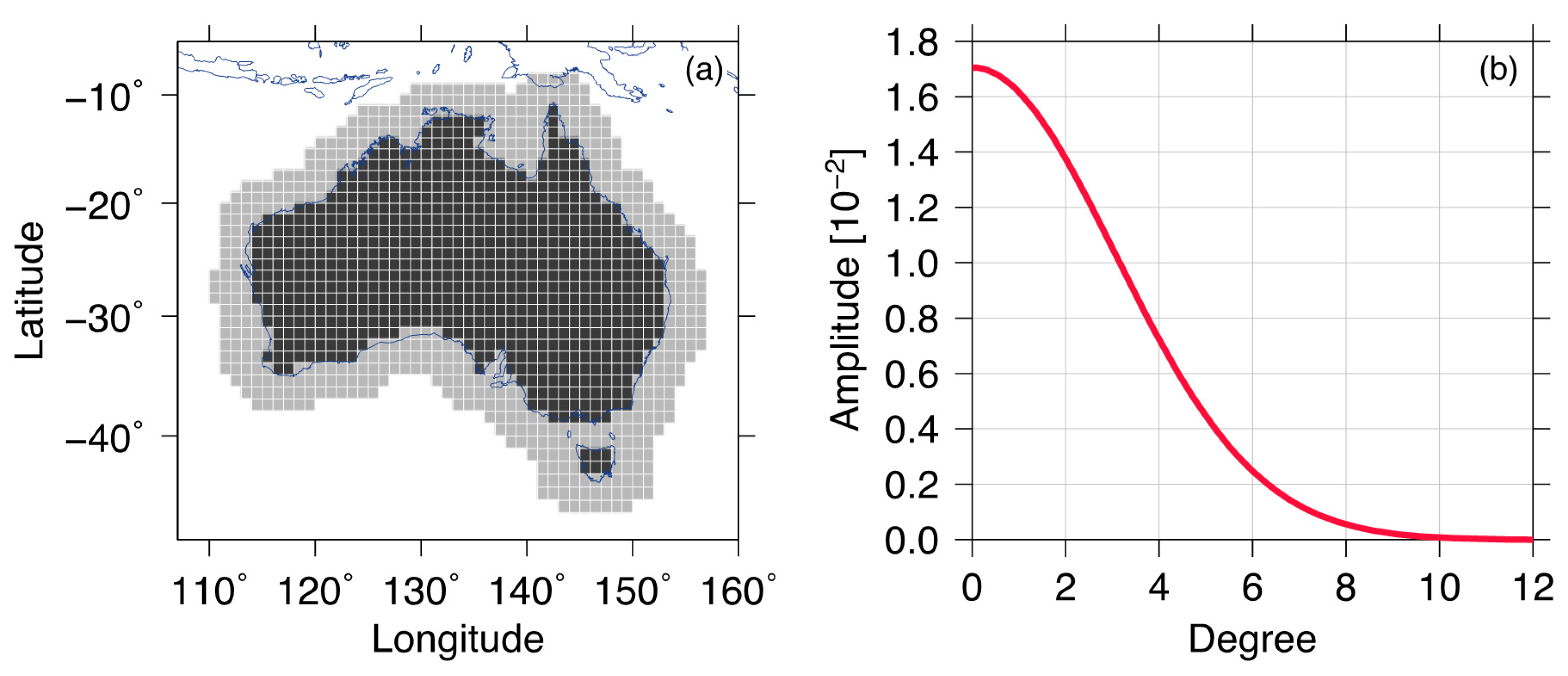In this case, $G$ is approximately the convolution operator associated with Gaussian smoothing. Using the continent of Australia as an example, we divide it into 1 × 1 degree pixels, including regions that extend 400 km into the oceans. Figure 1a shows grid points for both $\widehat{m}$ and $d_{obs}$ and black and gray pixels represent land and ocean grid points, respectively. We build the convolution operator G based on the Green function representing 400 km Gaussian smoothing for a unit mass (Figure 1b). Thus, elements of G, $g_{ij}$, are values shown in Figure 1b determined by the angular difference between ith and jth grid points.

$\widehat{m}$ can be estimated by minimizing the squared misfit:

$$\widehat{m}={\left(G^{T}G\right)}^{-1}{G}^T{d}_{obs}$$

(2)

but generally, this estimation problem is ill-posed because it is a downward continuation of the smoother gravity field at satellite altitude to Earth’s surface where the sources are located. To stabilize the solution, a regularization parameter ${\lambda }_r$ [17] can be used:

$$\widehat{m}={\left(G^{T}G+{\lambda }_{r}I\right)}^{-1}{G}^T{d}_{obs}$$

(3)

where $I$ is an identity matrix. The regularization parameter can be determined empirically or objectively with the L-curve method (e.g., [18]).

In this study we include a penalty that seeks to minimize spatial gradient (steepness) in the cost function [19]. This regularizes the problem and suppresses noise amplified as a result of the deconvolution. The steepness can be represented using the gradient of two surface mass loads. For example, for steepness between the first surface mass load, ${\widehat{m}}_1$, and others (${\widehat{m}}_2, {\widehat{m}}_3,\dots {\widehat{m}}_N)$, $D_1$ matrix can be constructed:

$$D_1=\left[\begin{array}{cc}\begin{array}{cc}-1/r_{12}& 1/r_{12}\\ -1/r_{13}& 0\end{array}& \begin{array}{cc}0& \cdots \\ 1/r_{13}& \cdots \end{array}\\ \begin{array}{cc}⋮& ⋮\\ -1/r_{1N}& 0\end{array}& \begin{array}{cc}\ddots & \cdots \\ \cdots & 1/r_{1N}\end{array}\end{array}\right]$$

(4)

in which $r_{1n} \left(n=2,3,\dots N\right)$ is the distance between the first and nth mass load. Therefore, steepness between the first mass load and all others is $D_1\widehat{m}$. Similarly, a steepness matrix ($D_2$) between the second and all other mass loads can be constructed and similarly for loads in all pixels. We define matrix $D$ considering all:

$$D={\sum }_{n=1}^N{D}_n$$

(5)

Including the steepness, the least squares solution is:

$$\widehat{m}={(G^{T}G+\lambda W)}^{-1}{G}^T{d}_{obs}$$

(6)

where $W=D^{T}D$ and $\lambda$ is a regularization parameter (different from ${\lambda }_r$ in Equation (3)). Larger value of $\lambda$ will suppress more noise but the estimate will be smoother. We empirically determine $\lambda$ in the next section.

Estimated $\widehat{m}$ over oceans (${\widehat{m}}_O)$ via Equation (6) includes three sources: ocean mass signal determined by self-attraction and loading (SAL) effects [12], residual ocean dynamic effects after applying atmospheric and ocean de-aliasing (AOD) fields from numerical models [20] and spurious leakage from terrestrial water mass load (${\widehat{m}}_L$). Terrestrial water mass loads cause leakage into oceans and at the same time, leakage into land by oceanic mass loads is also present. In general, the leakage into the oceans is much larger than leakage onto land. Considering both leakage effects is complicated. In this study, we only attempt to suppress spatial leakage from land to oceans by assuming that ${\widehat{m}}_O$ is zero. This constraint effectively ignores local ocean signals. It can be realized via an additional linear relationship:

$$H\widehat{m}=0$$

(7)

where $H$ is ones for ocean elements in ${\widehat{m}}_O$ and zeros elsewhere. This linear relationship can adjust ${\widehat{m}}_L$ by constraining ${\widehat{m}}_O$ to be zeros. The result is estimation of leakage corrected terrestrial mass loads.

Equation (6) can be modified by including Equation (7) in the cost function and the two equations must be solved simultaneously by combining them into the matrix form (see Section 3.10. in [21]):

$$\left[\begin{array}{cc}{G}^{T}G+\lambda W& H^T\\ H& 0\end{array}\right]\left[\begin{array}{c}\widehat{m}\left(t\right)\\ \widehat{n}\left(t\right)\end{array}\right]=\left[\begin{array}{c}{G}^{T}d{\left(t\right)}_{obs}\\ 0\end{array}\right]$$

(8)

where $\widehat{n}$ is a null parameter. We finally obtain the equation for $\widehat{m}$, which refers to an inversion solution, representing a constrained deconvolution of the GRACE data. We have yet to determine a useful value for the regularization parameter:

$$\left[\begin{array}{c}\widehat{m}\left(t\right)\\ \widehat{n}\left(t\right)\end{array}\right]={\left[\begin{array}{cc}{G}^{T}G+\lambda W& H^T\\ H& 0\end{array}\right]}^{-1}\left[\begin{array}{c}{G}^{T}d{\left(t\right)}_{obs}\\ 0\end{array}\right]$$

(9)

3. Synthetic Experiment in Australia

We apply Equation (9) to estimate surface mass loads over Australia using synthetic GRACE data. For surface mass load, surface water storage from Global Land Data Assimilation System (GLDAS) is used [22]. Surface water storage includes components of soil moisture, snow, and canopy water. Ocean dynamic effects are nominally corrected in GRACE data processing but residual ocean bottom pressure (OBP) signals, which may cause leakage contamination from oceans to land, may remain. We consider such effects using average ocean bottom pressure from CSR [23], GSFC [24] and JPL [25] mascons. Variations of total surface water storage and residual ocean dynamic effects are converted to SH coefficients up to degree and order 60. We also include GRACE noise, taking it to be the difference between GRACE data and smoothed GRACE data [6]. This difference field includes GRACE noise, which likely dominates spatially high frequency components, but it may also include some GRACE signal. The residual signal can be additionally separated from noise using Empirical Orthogonal Functions (EOF) [6]. The synthetic GRACE data is reduced by conventional GRACE data reduction methods, applying a de-correlation filter [9] and 400 km Gaussian smoothing.

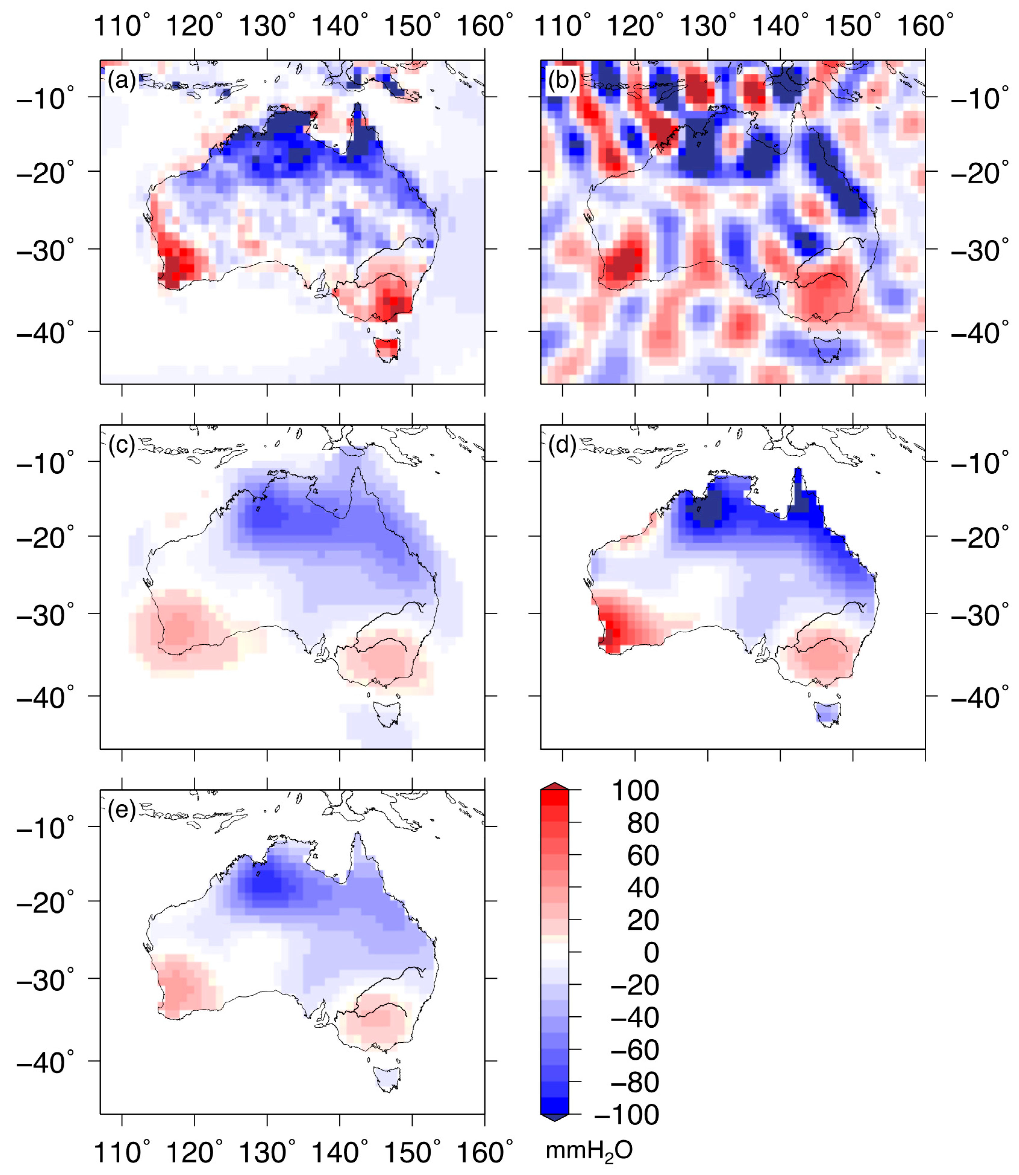
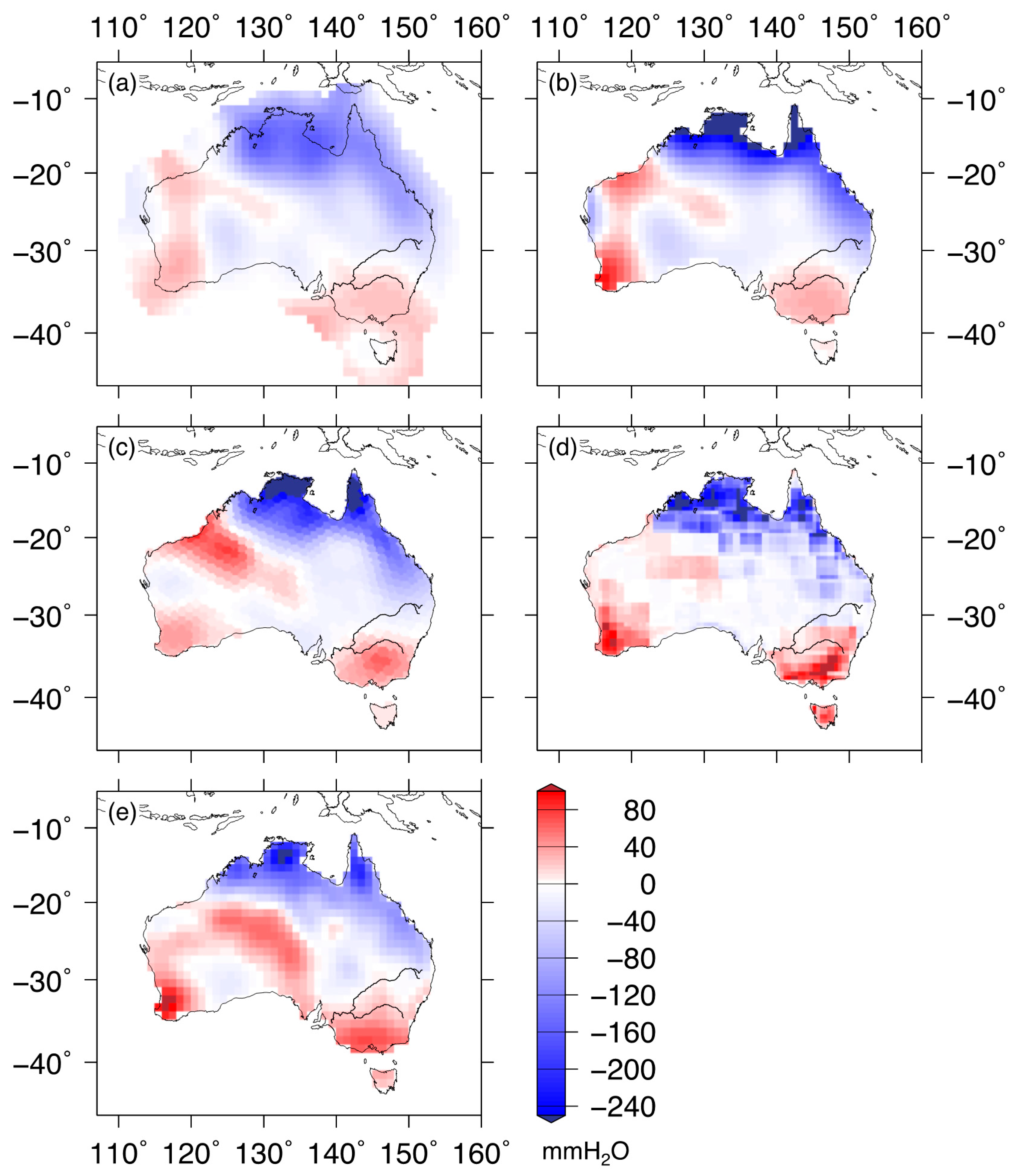
Figure 2a shows GLDAS surface mass loads over Australia and residual OBP for September 2005 and Figure 2b shows synthetic GRACE data, the sum of surface mass load shown in Figure 2a and estimated GRACE noise after applying decorrelation filter. GRACE noise is predominant in the synthetic GRACE data. Figure 2c shows ‘reduced’ surface mass load from synthetic GRACE data after applying a de-correlation filter and 400 km Gaussian smoothing. This is surface water mass load as in a conventional GRACE estimate. The mass load field is global but we only consider Australia and the surrounding 400 km of oceans. Spatial leakage of terrestrial signals into the oceans is evident, leading to reduced signal strength over land along the coast.

Figure 2d shows $\widehat{m}$, in Equation (9) estimated from Figure 2c as $d{\left(t\right)}_{obs}$ for a particular $\lambda =2\times {10}^5$, which was chosen by varying λ, and seeking the best agreement based on the regression coefficients between synthetic surface mass load (modeled by GLDAS) and estimated surface mass loads, $\widehat{m}$, and the root mean squared (RMS) difference between the two.

Table 1. Mean root mean squared (RMS) values with 95% confidence intervals and regression coefficients with coefficients of determinant between GLDAS and estimates surface mass loads from January 2003 to August 2016. Surface mass loads are estimated by different amounts of Gaussian smoothing (300, 400 and 500 km) and varying λ of inversion ($1\times {10}^5$, 2$\times {10}^5$ and $3\times {10}^5$).

	Gaussian			Inversion
	300 km	400 km	500 km	$1\times {10}^5$	$2\times {10}^5$	$3\times {10}^5$
RMS (mm)	31.64 ± 11.31	32.87 ± 12.45	35.15 ± 14.31	35.23 ± 11.58	31.87 ± 9.72	31.08 ± 9.36
Regression Coefficient	0.51 (r2 = 0.55)	0.41 (r2 = 0.55)	0.34 (r2 = 0.53)	0.72 (r2 = 0.52)	0.64 (r2 = 0.55)	0.58 (r2 = 0.55)

shows mean RMS and regression coefficients from Equation (9) with varying λ and different amounts of Gaussian smoothing during the entire period (January 2003–August 2016) of synthetic data. We determine $\lambda =2\times {10}^5$ to estimate $\widehat{m}$ because the regression coefficient is larger than any value from Gaussian smoothing while the RMS difference is close to the case of 300 km Gaussian smoothing, which provides the smallest RMS among Gaussian smoothing. Smaller λ provides a larger regression coefficient but simultaneously larger RMS difference. Estimated loads from Equation (9) with $\lambda =2\times {10}^5$ (Figure 2d) are closer to GLDAS fields relative to those in Figure 2c. For example, large leakage into the oceans is found in South Western and North Eastern Australia in Figure 2c and signal leaking to the oceans is moved back to the continent in Figure 2d. Estimated loads in Tasmania are evidently different from GLDAS loads due to its small spatial scale and the presence of large GRACE noise (shown in Figure 2b).

Figure 2e shows $\widehat{m}$ from Equation (6) without considering the constraint that ${\widehat{m}}_O$ are zeros, which is realized in Equation (7). The estimated surface mass loads shown in Figure 2e are similar to Figure 2c, the case of 400 km Gaussian smoothing. The comparison between Figure 2d,e clearly exhibits effect of the leakage correction in Equation (9), incorporating the constraint.

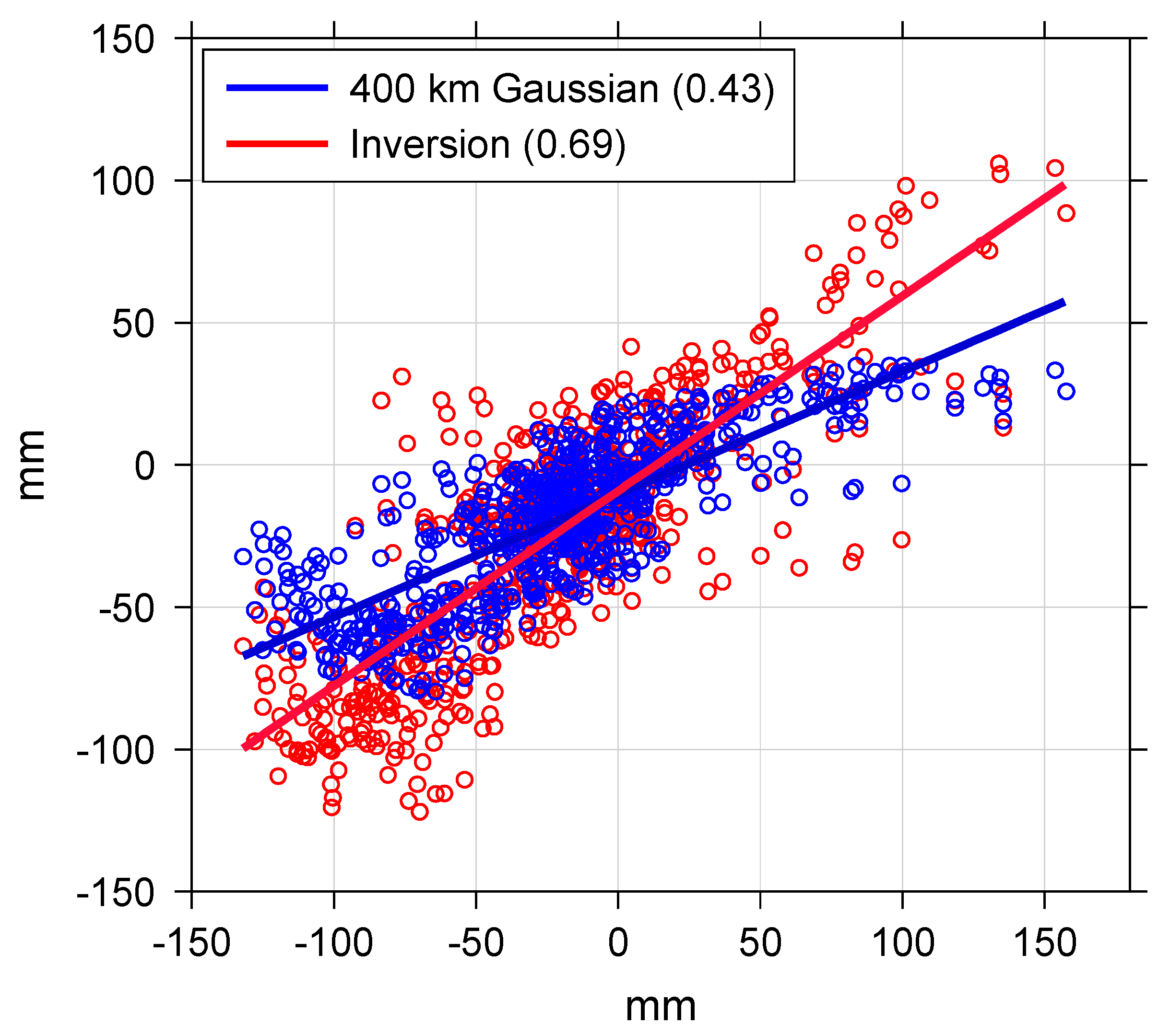
Figure 3 shows scatter plots between GLDAS and estimated surface mass loads from 400 km Gaussian smoothing (blue) and inversion (red) shown in Figure 2c,d, respectively. The linear regression coefficient from inversion (0.69, r² = 0.68) is much higher than that from Gaussian smoothing (0.43, r² = 0.65), with higher significance determined by the coefficient of determination, r². The RMS value from inversion (28.56 mm) is also much lower than that from 400 km Gaussian smoothing (32.78 mm).

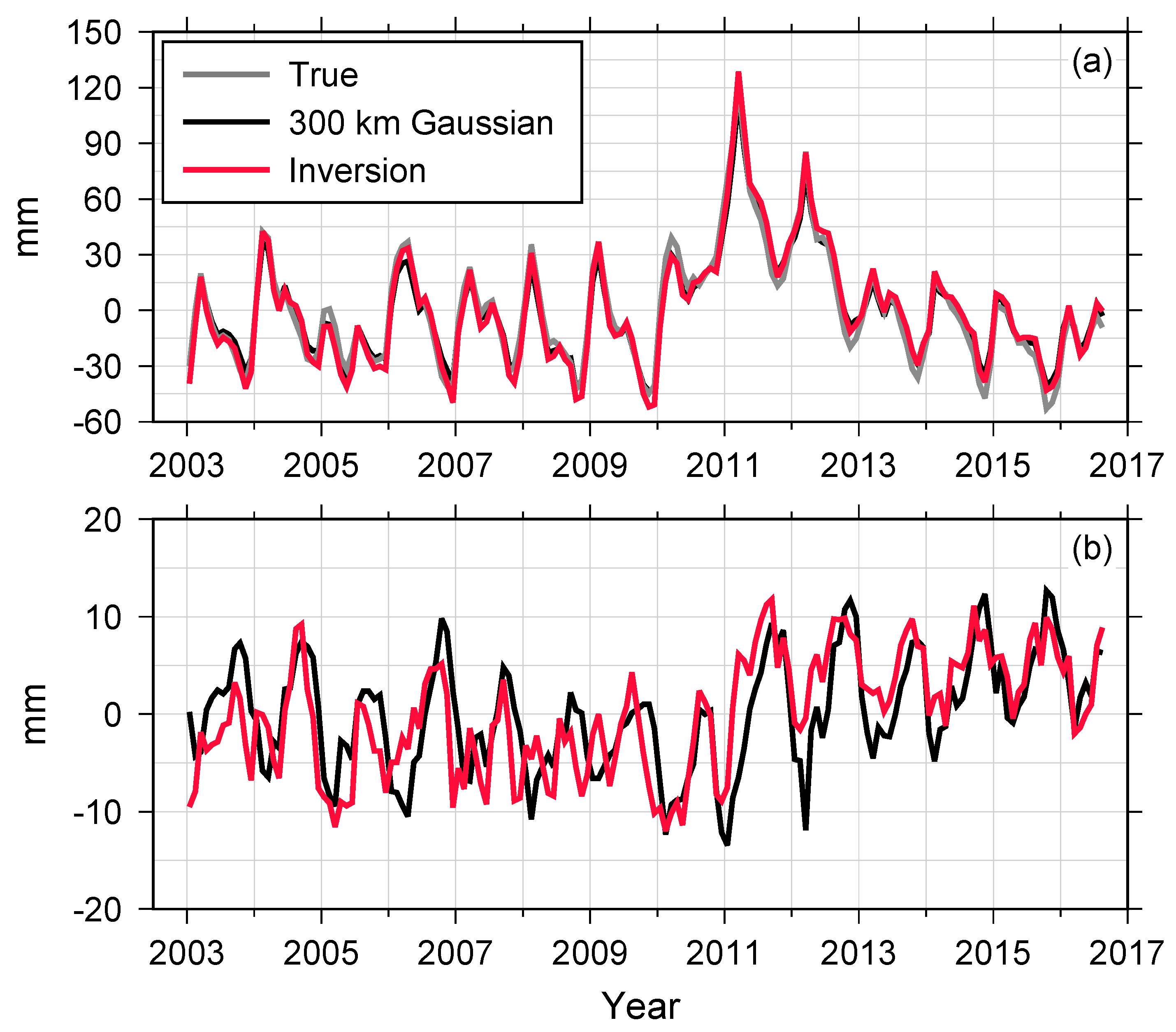
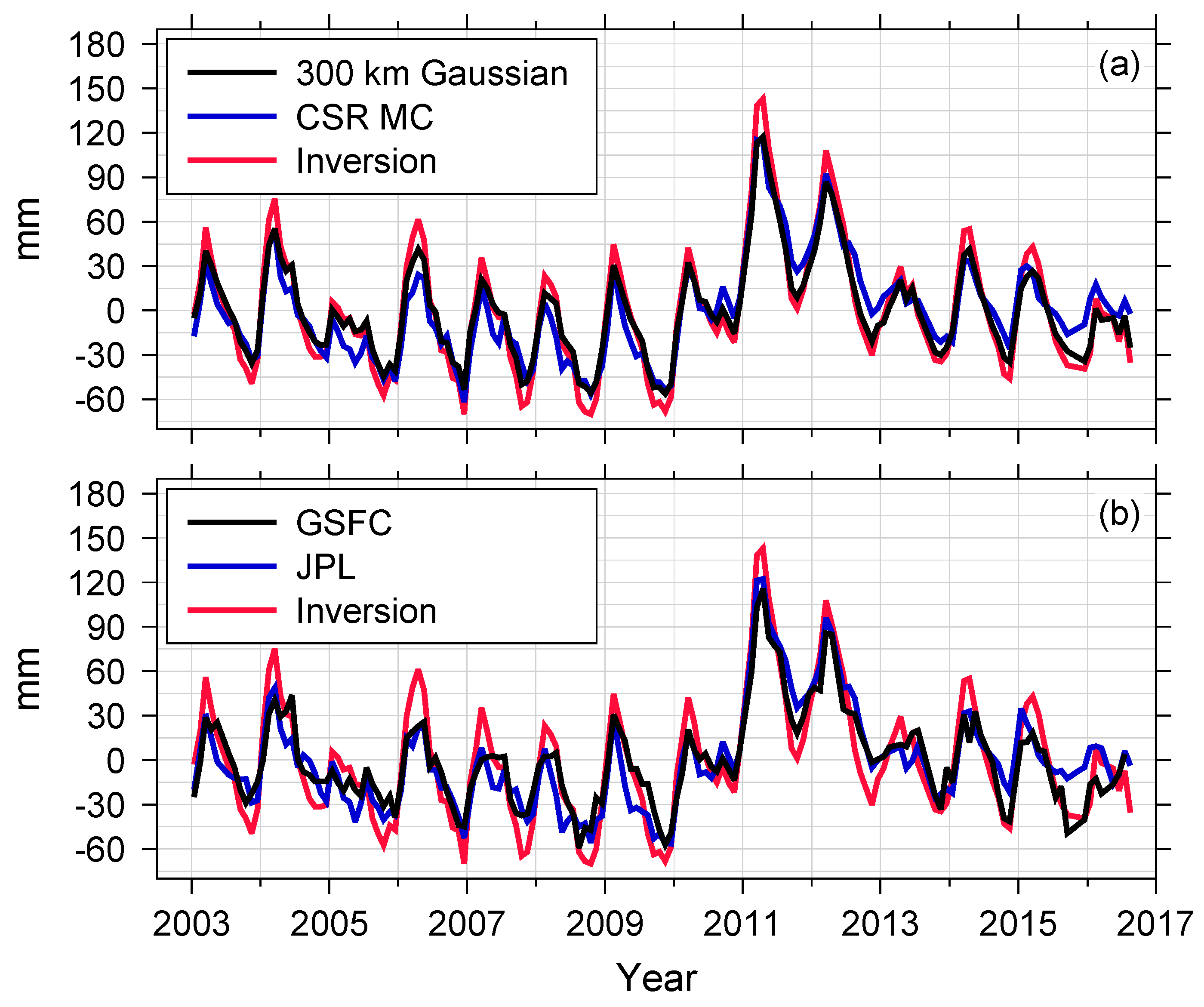
Because Gaussian smoothing with a 300 km length scale is superior to other choices shown in Table 1, we compare terrestrial water storage (TWS) estimates from Equation (9) for the 300 km case. Gray, black and red lines in Figure 4a show mean terrestrial water storage (TWS) time series over Australia associated with GLDAS, 300 km Gaussian smoothing and Equation (9) respectively. Both red (inversion) and black lines (300 km Gaussian smoothing) are close to GLDAS (gray) and similar to one another. As shown in Figure 4b, there are similar differences between estimates and GLDAS loads. This occurs because the sign of leakage differs across the continent. The sign is negative in North Australia and positive in the south as shown in Figure 2c. They tend to cancel in a continental scale average in this synthetic experiment. Cancellation would not be as important for real GRACE data as discussed in the next section.

The synthetic data experiment shows that constrained deconvolution, via Equation (9), with proper choice of λ, is superior to ordinary SH estimates subjected to Gaussian smoothing. TWS changes are closer to GLDAS values by suppressing leakage into the oceans, but they preserve TWS spatial patterns evident in the original SH solutions.

4. TWS in Australia

We now use observed GRACE data (CSR RL06 from January 2003 to August 2016) with Equation (9) to estimate TWS change in Australia. Initially we used the λ value determined from the synthetic data experiment but subsequently modified it as discussed shortly. Glacial isostatic adjustment is corrected by a model prediction based on ICE-6G_C ice thickness history and VM5a radial viscosity profile [26], although its effect is very small in Australia. North-south stripes are removed by a decorrelation filter [9]. Figure 5a shows surface mass loads for September 2005, the same month as the synthetic data experiment (Figure 2), including 300 km Gaussian smoothing. Spatial leakage into the oceans is evident. Pixels are 1 × 1 degrees over Australia out to 400 km from the coast, as in the synthetic experiment.

Comparing GLDAS-derived (Figure 2c) and GRACE fields (Figure 5a) shows that GLDAS has likely underestimated the magnitude of Australian TWS change. A larger TWS signal relative to GLDAS is evident also in Figure 6a, where continent-wide variations from GRACE are larger than GLDAS values.

The value for $\lambda$ is chosen to suppress noise but it also suppresses signal, so must depend upon the signal to noise ratio. From the synthetic data experiment $\lambda =2\times {10}^5$ but if the signal level is higher, relative to GLDAS used in the synthetic experiment, then a smaller value may be appropriate. The RMS value from the black line in Figure 6a is about 1.3 times larger than that of the black line in Figure 4a. The discrepancy reflects lower signal strength in GLDAS relative to GRACE. Therefore, we returned to the synthetic experiments to adjust GLDAS variations by a factor of 1.3 to compensate for the underestimate of GLDAS. From this, we selected an optimum $\lambda =1\times {10}^5$.

Figure 5b shows estimated TWS change from Equation (9). Large TWS signals appear along coastal areas relative to conventional Gaussian smoothed estimates (Figure 5a). The red line in Figure 6a shows resulting continent-wide TWS variations. Variability in black and red lines in Figure 6a is very close to each other (correlation coefficient, 0.99) while peak-to-peak changes in the red line are much larger than the black line. An additional comparison is shown in Figure 6a with CSR mascon solutions [23] (blue line). In general, the CSR mascon solutions show smaller peak-to-peak variations relative to the Equation (9) solution and they are rather close to the case of Gaussian smoothing. We also compare GSFC [24] and JPL [25] mascon solutions with inversion (Figure 6b). Smoothing effects in JPL mascon solutions were corrected by applying gain factors [27]. Similar to CSR mascon solutions, GSFC and JPL mascon solutions also show smaller TWS variations than the Equation (9) solution. Figure 5c–e show TWS from CSR, JPL and GSFC mascons respectively, for the same month as in Figure 5a,b. TWS spatial patterns are different from one another while the CSR mascon solution (Figure 5c) is close to the inversion estimate (Figure 5b).

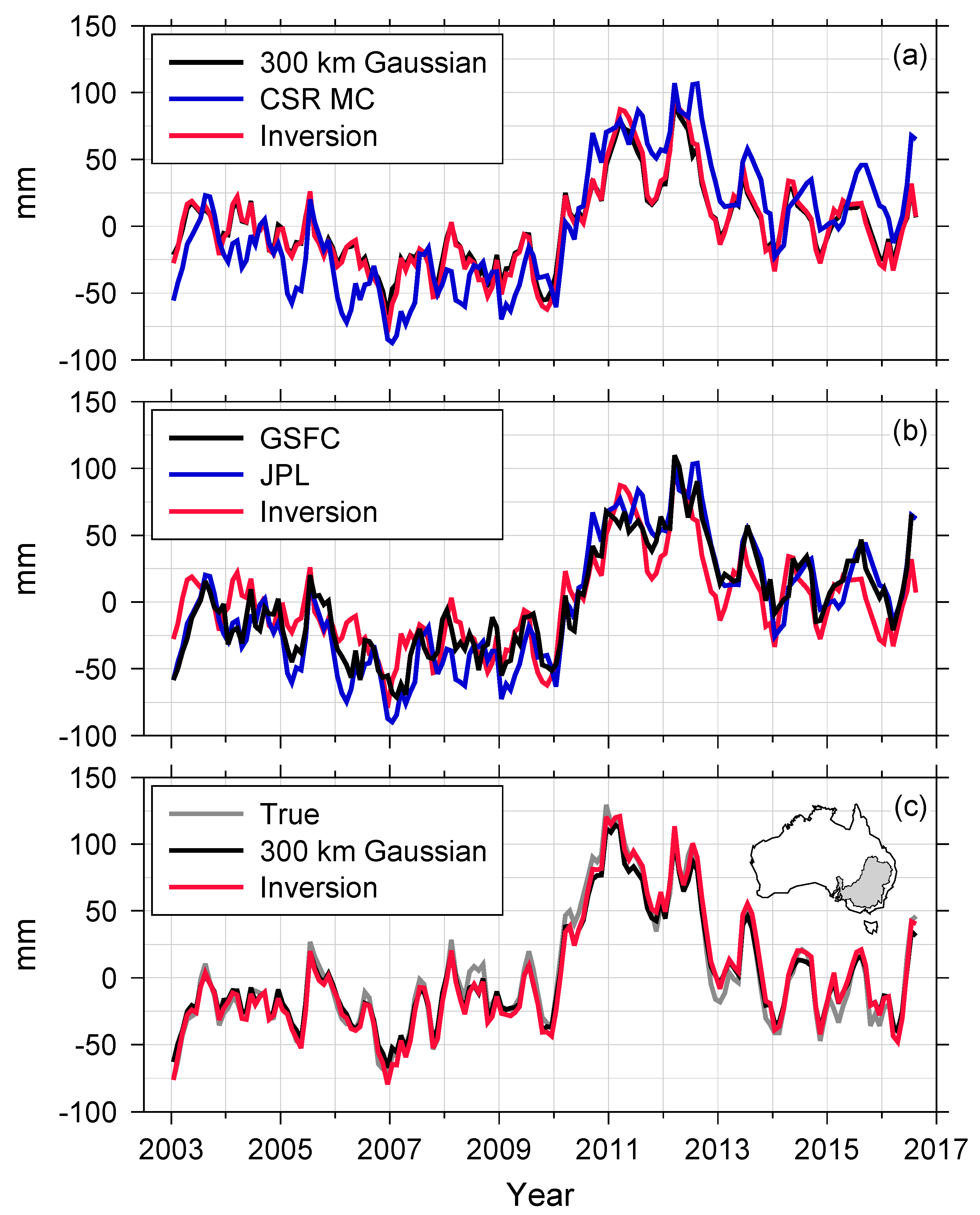
We further compare TWS from Gaussian smoothing, mascons and inversion at basin scales to examine their uncertainty. First, we choose the Timor Sea Basin, located on the north coast of Australia, showing large TWS variations. It is a good choice for studying leakage effect and corrections among the three methods. Figure 7a shows TWS variations from the three methods. Both CSR mascon (blue) and inversion (red) provide similar TWS variations while their peak-to-peak variations are much larger than those from Gaussian smoothing (black). This indicates that the mascon and Equation (9) solutions suppress leakage effects in basins near the oceans. Similar results are also found comparing JPL mascon (blue) and inversion (red) in Figure 7b. The GSFC mascon solution (black), however, evidently underestimates TWS variations relative to inversion and other mascons. Figure 7c shows a synthetic experiment for the Timor Sea Basin, where inversion (Equation (9)) TWS (red) is much closer to GLDAS (gray) than the Gaussian estimate (black). Some discrepancies between red and gray curves are evident in Figure 7c, indicating leakage may not be completely corrected using Equation (9). Despite this likelihood in the case of real GRACE data shown in Figure 7a, Equation (9) estimates removed much of the leakage error associated with Gaussian smoothing. A similar limitation appears in mascon solutions, which show very similar TWS variations in Figure 7a,b.

We apply the same analysis to the Murray Darling Basin, located in the continental interior. It differs from the Timor Sea basin in distance from the ocean, with small TWS variations over a basin of much larger size. The Murray Darling and Timor Sea Basin areas are 1.15 × 10⁶ km² and 0.62 × 10⁶ km² respectively. Figure 8a shows TWS variations over the basin from Gaussian smoothing (black), CSR mascon (blue) and Equation (9) inversion (red). Inversion and Gaussian smoothing provide very similar TWS variations because the effect of smoothing should be small in a large interior basin. The same conclusion can be found in the synthetic experiment (Figure 8c): both Gaussian smoothing and Equation (9) show similar variations as GLDAS. However, mascons (blue line in Figure 8a and black and blue lines in Figure 8b) are distinctly different. The cause of this discrepancy is unknown but it suggests that CSR, GSFC and JPL mascon solutions may not perform well in certain situations. Similar results are found in other basins in Australia, such as the Lake Eyre Basin.

5. Conclusions

We have developed a constrained deconvolution method to estimate surface mass loads from GRACE data. Noise is suppressed by minimizing steepness of the estimated surface mass loads in the cost function. Signal leakage from land to oceans is suppressed by constraining ocean signals to be approximately zero. Testing this method using synthetic GRACE data shows results that are superior to Gaussian smoothing.

Using this method, we estimate surface mass loads over Australia from GRACE data. As in the synthetic case, estimates show higher signal strength near the coast relative to Gaussian smoothing but retain high correlation with Gaussian smoothing estimates. TWS variations are also compared with those from CSR, GSFC and JPL mascon solutions. In the examples studied here, mascon solutions suppress leakage into the oceans but show smaller peak-to-peak variation and may be problematic in interior basins with small signals.

The constrained deconvolution method should be useful in geographical regions adjacent to oceans or lakes to suppress leakage error. Calibration of λ for particular problems is necessary. We show that it likely depends both on signal strength and probably also, to some extent, on pixel size. However, the process should be straightforward, using methods similar to those in the synthetic data experiment. Additional estimates incorporating other data types, such as GPS loading observations, would be particularly useful to enhance spatial resolution while reconciling leakage problems.