Article

Towards Predictive Modeling of Sorghum Biomass Yields Using Fraction of Absorbed Photosynthetically Active Radiation Derived from Sentinel-2 Satellite Imagery and Supervised Machine Learning Techniques

by
Ephrem Habyarimana
1,*,
Isabelle Piccard
2,
Marcello Catellani
1,3,
Paolo De Franceschi
1 and
Michela Dall’Agata
1
1
CREA Research Center for Cereal and Industrial Crops, Bologna 40128, Italy
2
Vlaamse instelling voor technologisch onderzoek N.V., MOL 2400, Belgium
3
Department for Sustainability, Italian National Agency for New Technologies, Energy and Sustainable Economic Development (ENEA), Rotondella (MT) 75026, Italy
*
Author to whom correspondence should be addressed.
Agronomy 2019, 9(4), 203; https://doi.org/10.3390/agronomy9040203
Submission received: 23 March 2019 / Revised: 13 April 2019 / Accepted: 18 April 2019 / Published: 20 April 2019
(This article belongs to the Special Issue Remote Sensing Applications for Agriculture and Crop Modelling)

Abstract

:
Sorghum crop is grown under tropical and temperate latitudes for several purposes including production of health promoting food from the kernel and forage and biofuels from aboveground biomass. One of the concerns of policy-makers and sorghum growers is to cost-effectively predict biomass yields early during the cropping season to improve biomass and biofuel management. The objective of this study was to investigate if Sentinel-2 satellite images could be used to predict within-season biomass sorghum yields in the Mediterranean region. Thirteen machine learning algorithms were tested on fortnightly Sentinel-2A and Sentinel-2B estimates of the fraction of Absorbed Photosynthetically Active Radiation (fAPAR) in combination with in situ aboveground biomass yields from demonstrative fields in Italy. A gradient boosting algorithm implementing the xgbtree method was the best predictive model as it was satisfactorily implemented anywhere from May to July. The best prediction time was the month of May followed by May–June and May–July. To the best of our knowledge, this work represents the first time Sentinel-2-derived fAPAR is used in sorghum biomass predictive modeling. The results from this study will help farmers improve their sorghum biomass business operations and policy-makers and extension services improve energy planning and avoid energy-related crises.

1. Introduction

Sorghum (Sorghum bicolor (L.) Moench) is a cereal with a C4 carbon fixation (the Hatch—Slack pathway) cultivated mainly for food, feed, forage, and fuel [1]. Sorghum grain was historically used for human consumption in developing countries but, because it is gluten-free, with low glycemic index and high contents of macronutrients and antioxidants, its utilization as food extended worldwide.
There are several types of sorghum. Grain sorghums are generally shorter (usually having recessive alleles at three of the four Dw genes) than biomass sorghums (having recessive alleles at two Dw genes at most), and have been selected to have the grain as the primary sink for photosynthates. Biomass sorghum of biofuel production interest was used in this work and includes dual purpose (showing high grain and biomass yields), forage, sweet, and biomass sorghum types [2,3,4,5]. The sweet sorghum type translocates photosynthates to the seeds and stem; their stems are juicy (d recessive to D) instead of dry and sweet (x recessive to X) instead of nonsweet [6]. Sweet sorghums are high biomass and sugar yielding crops, and were traditionally bred for syrup or molasses production. Forage sorghum’s main characteristics include digestible fiber and low lignin content, while biomass and dual purpose sorghums include high biomass yielding genotypes with high contents of structural carbohydrates, which are being developed for feedstock production [5]. Sorghum can therefore supply several products including starch, soluble sugars, structural carbohydrates, and organic matter for energy production purposes. Several countries worldwide, including in higher latitudes [7], are increasingly developing dedicated biomass sorghums in response to the pressing issue for nations to get independent of foreign energy sources and to cut carbon emissions into the atmosphere [7,8]. As a biofuel-dedicated biomass business, growing sorghum will have to meet critical requirements of high and cost-effective productivity of biobased commodities.
Crop yield forecasting is one of the most important strategies in agriculture, which enables sustainable development and helps avoid famines and shortages in several commodities [9,10,11,12]. In industrialized countries, crop yield forecasting provides data to governmental structures, companies, and farmers, which results in strategic advantages such as the rationalization of policy adjustments, price predictions and stabilization, efficient agricultural trade, and simplification of business operations particularly through planning harvest and delivery of the produce, better deployments of machineries and logistics, and a better management at the end user level (e.g., bioreactor owner).
Conventionally, and particularly in developed countries, the information on crop production is collected and disseminated through field surveys and censuses, but this system is rather costly and associated with significant uncertainties [13]. Using satellite imagery resulted in a superior solution [14,15,16]. Remote sensing data has been used for many years to build operational crop yield forecasting systems like the FAO’s Global Information and Early Warning System (GIEWS). The use of remote sensing satellite data for crop yield forecasting is further motivated by wide coverage, near-real time delivery of data and products, and the ability to provide vegetation indicators at low cost. Many studies have shown that forecasting models based on remote sensing data can give similar or better performance comparing to the more sophisticated physiological crop growth models [13,17,18,19].
The use of remote sensing parameters as proxies for biomass yields was documented in previous works. Normalized difference vegetation index (NDVI), leaf area index (LAI), and fAPAR (fraction of absorbed photosynthetically active radiation) are among the most frequently used parameters [14,16,20]. Recently, the use of biophysical parameters, such as fAPAR, gained more attention relative to using vegetation indices [21,22]. Biophysical parameters reflect the state of the crops more adequately and thus could be better suited for predicting crop yield and production [15,23,24]. fAPAR is defined as the fraction of radiation absorbed by the green vegetation elements in the 400 to 700 nm spectral domain under specified illumination conditions [25]. It is directly linked to photosynthesis, and therefore expresses a canopy’s energy absorption capacity [26]. fAPAR values range from 0 to 1, indicating, respectively, bare soil and fully crop covered soil.
Most of the aforementioned studies were focused on common field crops like corn, wheat, barley or soybeans [16,20,27,28,29,30]. A few studies dealt with remote sensing-based yield monitoring and prediction [16] in sorghum. For instance, Shafian et al. [31] described the use of unmanned aerial vehicle-based remote sensing to investigate sorghum crop physiological properties. Yang et al. [32] combined airborne digital videography with ground sampling, regression analysis, and image processing to map spatial sorghum grain yield variability within fields and across the cropping season. Johnson [16] presented a comprehensive assessment of the correlations between commonly used Moderate Resolution Imaging Spectroradiometer (MODIS) products and field crop yields, including sorghum, and used these correlations for biomass yield estimation and prediction.
In most studies, however, remote sensing-based biomass yield estimation or prediction makes use of low- or medium-resolution satellite images from sensors such as SPOT-VEGETATION [14,15,23,24] or MODIS [16]. These satellite products have a coarser spatial resolution (250 to 1000 m) compared to the data collected from the two Sentinel-2 satellites in this work (10-m spatial resolution). With the launch of the Sentinel-2 constellation of satellites the overpass frequency (five days and locally even two to three days) the temporal resolution is nearly as good as for SPOT-VEGETATION and MODIS satellites (one to two days). The high spatial resolution of the Sentinel-2 images is an important asset when monitoring crops in agricultural regions characterized by many small fields. To our knowledge no previous studies assessed the efficiency of high resolution Sentinel-2-derived fAPAR data in predicting within-season biomass sorghum yields, and this paper is therefore aimed at addressing this gap.
Deriving yield information from satellite imagery has shown promising results but this technology is not extensively applied across farmers and crop species worldwide [27,28,29]. In this work, we developed models for within-season prediction of annual and perennial sorghum biomass yields in Emilia-Romagna, Italy, based on fAPAR measurements from Sentinel 2A and Sentinel 2B satellite images on 42 mostly full-fledged commercial sorghum fields. We used machine learning algorithms to create yield prediction equations. These equations can be implemented in decision support systems to allow farmers and/or farming stakeholders to predict biomass yields from sorghum fields of interest early on in the cropping season. This information is very helpful to efficiently schedule fleets of harvesting machinery, transport vehicles, and storage facilities. The fAPAR-derived predictive models for biomass yields can also be implemented by extension services and policy-makers for several purposes, including the possibility to anticipate potential biomass availability and plan ahead, to avoid specific crises such as fuel shortage.

2. Materials and Methods

2.1. Trial Set-Up

Forty-two demonstration trials were run in this work, 23 and 19 of which were evaluated in 2017 and 2018, respectively. In 2017, the experimental sites were located in Conselice, Nonantola, Mirandola, and Anzola dell’Emilia, in the Italian region of Emilia Romagna (Table 1, Figure 1), while in 2018 the sites were established in Anzola, Mirandola, and Conselice (Figure 1, Table 1). The experimental sites were strategically selected to maximize extension impact by conducting most of the trials in the farmers’ fields. The experimental fields in Mirandola and Conselice belonged to respective two big farming cooperatives with more than 2000 members each. In Nonantola, the fields belonged to individual farmers, while in Anzola the fields were established in the experimental station of the Council for Agricultural Research and Economics (CREA). The fields were generally of big size relative to plot sizes commonly used under standard experimental settings [1] in order to serve the purpose of demonstrative pilots with the objective of transferring into the production environment the technology of sorghum crop monitoring using satellite imagery. The fields areas ranged from 0.06 ha to 50.00 ha, with a mean and median of 5.70 ha and 1.10 ha, respectively. All the fields were planted with biomass sorghums including biomass per se (high tonnage), sweet, forage, and dual purpose types. One-grain sorghum trials were established in Anzola in 2017, but it was not included in this work in virtue of a different kind of experiment management and a diverse market of the grain sorghum produce relative to biomass sorghum. Thirty-five out of the 42 trials were sown with a single genotype of Sorghum bicolor (annual), while the 17IT_mat was sown with a diversity panel of 228 biomass Sorghum bicolor genotypes, and six (15R17, 16R17, 16R18, 15R18, 17R18, and 17US_mat) of the trials installed in Anzola were made up of a diversity panel consisting of advanced perennial interploid biomass hybrids deriving from S. bicolor × S. halepense (SB × SH) crosses. The original SB × SH materials originated from The Land Institute (Salina, KS, United States of America). S. bicolor × S. halepense breeding strategy was amply detailed in Piper and Kulakow [33] and in Habyarimana et al. [1]. The 15R, 16R, 17R, and 17US_mat trials were sown in 2015, 2016, and 2017, respectively, meaning that regrowth-derived biomass was evaluated for the 15R, 16R, and 17R trials, while for the 17US_mat trial, the biomass evaluated in this study was produced from direct sowing.
Crop management followed local extension services guidelines and was well described in Habyarimana et al. [1]. Planting density was 26 (0.75 m spacing between rows; 0.052 m spacing of hills within row) plants per square meter for most (35) trials, and 13 (0.75 m spacing between rows; 0.10 m spacing of hills within row) plants per square meter for 15R, 16R, 17R, 17IT_mat, and 17US_mat trials. In terms of weather (Figures S1–S4), summer was generally dry across years and locations as expected. In 2017, all sites had relatively wet spring except in Anzola, while in 2018 spring was relatively wet in Anzola and Conselice, but dry in Mirandola.

2.2. Biomass Data Collection

Trials in Nonantola, Mirandola, and Conselice were harvested at industrial scale from end of August to late November, while all trials in Anzola were harvested end of November using a single-row chopper harvester. Our experience showed that postponing harvest to later times may increase the likelihood for lodging, which may lead to the crop touching the ground, adding grit to the biomass material and possibly reducing biomass quality; delayed harvest also leads to kernel loss and kernel quality deterioration particularly due to molds, insect, and bird damages. The trials were harvested according to two machinery options: forage chopper or swathing the material into windrows and then baling it in large square bales or large round bales. Chopped biomass was weighed immediately at harvest, while baled biomass was weighed when bales were transported to the bioreactor. Chopped and baled biomasses were supplied to private biogas and combustion bioreactors. From each field, a 1kg-composite sample was taken from the sold biomass at the time of shipment to the end user in order to determine the dry mass content in the commercialized produce and calculate the dry biomass yield for each entire field that will be used in modeling. For the diversity panels, samples were taken from each genotype. Fresh samples were weighed and dried at 80 °C to constant weight in a forced air oven. The fresh and dry weights of the samples, and the fresh weight of the entire field’s harvest, were used to derive dry mass fraction of the fresh material and dry biomass yield of the entire field. For the diversity panel fields, the final yields integrated the contributions of the component genotypes.

2.3. Satellite Data Acquisition

For this study we used Sentinel-2 optical satellite imagery. The Sentinel-2 mission is based on a constellation of two satellites—Sentinel-2A and Sentinel-2B—both orbiting Earth at an altitude of 786 km, but 180 ° apart to optimize coverage and global revisit times. Swath width, i.e., the image width across the satellite path when scanning the Earth, is 290 km. As a constellation, the revisit time is 5 days. This means that the same spot over the equator is revisited every five days, and even faster at higher latitudes. Sentinel-2 data are acquired on 13 spectral bands in the VNIR (visible and near-infrared) and SWIR (short-wave infrared) range, of which four bands with a spatial resolution of 10 meters (blue, green, red, and near-infrared (NIR)), six bands at 20 meters (three red edge bands, a narrow NIR, and two SWIR bands), and three bands at 60 meters (a coastal aerosol, water vapor, and cirrus band). Spatial resolution refers to the surface area measured on the ground and represented by an individual pixel. Once the Sentinel data are acquired on-board, they are sent to ground and processed by a network of Processing and Archiving Centers. Next, all data products are united, archived, and disseminated online to the users by ESA’s Copernicus Space Component (CSC) Ground Segment via the CSC Data Access Coordinated System. To facilitate image transfer and use, the projected Sentinel-2 images are converted to tiles with a fixed size of 100 square kilometers, each of which is approximately 500 MB.
For this study, Sentinel-2A and Sentinel-2B images from tile 32TQQ (including pilots from Conselice) and 32TPQ (including pilots from Anzola, Mirandola, and Nonantola) were downloaded from ESA and processed by Vlaamse Instelling voor Technologisch Onderzoek N.V. (VITO). Processing included atmospheric correction with iCOR [34] and cloud and shadow detection using Sen2COR v2.5.5 (ESA-STEP, ESA, Paris, France). Biophysical parameters fAPAR, fCover, and leaf area index (LAI) were calculated from the top of canopy normalized reflectances following the BV-NET (tool for mapping surface and vegetation variables) method described by Weiss and Baret [35]. The BV-NET methodology is based on neural networks which are trained on a synthetic dataset of ~50,000 simulations using the PROSAIL (PROSPECT and SAIL radiative transfer models) model [36]. The BV-NET version used in this study was calibrated with green, red and near infrared bands, all having a spatial resolution of 10 meters. Sen2Cor and BV-NET are publicly available through ESA’s SNAP (Sentinel Application Platform, ESA, Paris, France) toolbox.
Previous studies such as Duveiller et al. [15], López-Lozano et al. [24], and Johnson et al. [16] illustrated the good performance of satellite derived fAPAR for estimating and predicting biomass yields of large field crops, including corn and sugarcane, which, together with sorghum, make-up the world’s three economically important C4 crops of the Poaceae family with similar growth habits [37]. We therefore decided to use fAPAR for this study as well. The fAPAR estimates generated with BV-NET from Sentinel-2A and 2B top of canopy reflectances over selected tiles in Emilia-Romagna had a spatial resolution of 10 meters and a temporal resolution of 5 days up to 2–3 days in those areas where the different satellite overpasses overlapped.
For monitoring the sorghum fields in this study “WatchITgrow” (Vlaamse Instelling voor Technologisch Onderzoek N.V., MOL, Belgium) was used. WatchITgrow is a web-based application for crop monitoring developed by VITO. It provides information on crop growth and development as well as possible anomalies derived from Sentinel-2 satellite images and weather data, and it allows the user to store all kinds of collected field data, such as planting and harvest dates and development stages, but also information on crop treatments such as fertilization, spraying, or irrigation. Prior to monitoring, the fields used in this study were geolocalized (Figure 1) using Field GPS (global positioning syatem) application for iPhone with a final field boundary correction using Google Earth. The field polygons were saved as kml files and then imported into WatchITgrow for monitoring. For each field, fAPAR or “greenness” maps were created (see example in Figure 2), and a growth curve was built, showing the evolution of the fAPAR values throughout the cropping season (see example in Figure 3). To build the growth curve the fAPAR values of all pixels within the field were averaged, thereby accounting for an inside buffer of ten meters (one pixel) in order to avoid capturing signals from neighboring fields or other objects. To correct for artifacts in the resulting fAPAR curve such as abnormally low fAPAR values due to undetected clouds, shadows or haze and to interpolate fAPAR values between subsequent acquisition dates, a Whittaker smoothing filter was applied on the curve [38,39].

2.4. Modeling Total Aboveground Biomass Yields

Thirteen models were assessed in this study to predict sorghum biomass yields. The models included partial least square discriminant analysis (PLS-DA), principal component analysis discriminant analysis (PCA-DA), neural network (NN), random forest (RF), support vector machine (SVM) with linear classifier (SVML), nonlinear kernel (SVML_G), radial basis kernel (SVM_R), radial basis kernel with polynomial basis kernel (SVM_P), neural network (NNET), eXtreme Gradient Boosting- xgbtree method (GBT), eXtreme Gradient Boosting- xgbDART method (GBD), eXtreme Gradient Boosting-xgbLinear method (GBL), simple linear model (LM), and Neural Network-neuralnet method (NLNET). The simple linear model was used as a benchmark to gauge the performance of the models implemented. The models evaluated in this work were selected based on their robustness as reported in previous studies [40].
The field-based daily interpolated fAPAR estimates extracted from WatchITgrow were converted to fortnightly fAPAR averages. In this study, preference was given to the use of fortnightly fAPAR data as major morphophysiological changes in crops also occur fortnightly [41]. In addition pilots established in experimental stations and in farmers’ fields were fortnightly visited at or close to the times the fAPAR images used in this work were acquired. This time management was also favorable and accommodated the busy schedules of farmers and scientists.
Six fortnightly fAPAR values registered from May to July—here referred to as six “days of year” (DOY), that is, DOY 135 and 150 in May, 165 and 180 in June, and 195 and 210 in July—were used as regressor variables in successive predictive modeling of sorghum biomass yields. May, June, and July are important months concerning the predictive modeling, mimicking the 1 to 2 months required to release yield predictions before harvest [42]; taking into account that biomass sorghum in the Mediterranean region is harvested from August to November.
The research questions addressed in this work are (1) how accurately can we predict the yield of a biomass sorghum field based of Sentinel-2-derived fAPAR profile early in the cropping season? (2) Which months and/or days-of-year best contribute useful information for predicting biomass yields in commercial sorghum fields? The solutions to the above problems were evaluated by solving the below linear model for n trials or experimental locations ( i = 1 , , n ) and p prediction times or days of year ( j = 1 , , p ). This model is represented by
y i = μ + j = 1 p x i j β j + e i
where μ is the overall mean, y i is the phenotypic observation (biomass yields) from field i , e i is the residual comprising all other nongenetic and environmental factors, x i j is the days of year covariates, and β j is the effect of the jth day of year covariate on y i [43]. Note that it is beyond the scope being presented here to identify and/or predict within-field yield variability for any potential applications. In addition, different sorghum types were combined in this study as they qualified for commercial aboveground biomass production and to mimic farming practices in the region of the study. We also assumed that the test region was homogeneous with respect to climatic conditions.
All statistical analyses were carried out using R software [44]. The predictive models were fitted using the caret R package. In this work, the “one standard error” rule of Breiman et al. [45] was implemented to avoid overfitting, and the caret built-in features were invoked to automatically choose the tuning parameters associated with the best performance of the regression routines. During data preparation, zero-variance regressors were removed and those remaining were centered and scaled in order to avoid regressors with zero or near-zero variance, which often constitute a problem as they behave as second intercepts in predictive models [40]. The dataset was randomly partitioned into training (80% of the entire dataset; 34 observations) and testing set (20% of the entire dataset; eight observations). The training set was used to run a cross-validation experiment to train and assess the models using a 10× repeated 5-random fold cross-validation (CV) iterations, rendering a total of 50 estimates of accuracy and prediction error; a large number of repetitions is expected to compensate for the high variance stemming from a reduced number of folds. Models were validated on the testing set which was an external test (validation) sample set needed so that the model performance can be characterized on data that were not used in the model training. The models were evaluated based on the prediction accuracy, the mean absolute error (MAE), and the mean absolute percentage error (MAPE). The MAE built within the repeated cross validation procedure (model calibration) was used to assess the variability (dependability) of the model performance. On the other hand, the MAE, MAPE, and accuracy obtained on the testing set were used to assess the model predictive ability. The MAPE allows us to compare the prediction of different dependent variables in different scales. The MAE measured the average magnitude of the errors in the set of predictions of biophysical variable values produced in this work, without considering their direction. It represented the average over the test sample of the absolute differences between prediction and actual observation where all individual differences had equal weight. The MAE was chosen for the model verification because it provides an unambiguous measure of the magnitude of the average error and is therefore more appropriate than the Root Mean Square Error (RMSE) for dimensioned evaluations of average model performance error [46]. The distribution of the 50 MAE estimates from the optimal cross-validated models was characterized using boxplot, while the comparison of mean accuracies across models and across prediction times was performed using Duncan’s test [47]. The importance of the regressor variables (useful prediction times) was determined using a 0 to 100 index, with 0 corresponding to no effect and 100 corresponding to the highest magnitude of the regressor’s importance. The accuracy was defined as the Pearson correlation coefficient between the predicted and the observed biomass yield values in the testing set [5]. From the computed accuracy, r-squared values can be derived in order to better compare, for each model, the proportion of the variance in the dependent variable that is predictable from the regressors.

3. Results

3.1. fAPAR Index Pattern Across Sorghum Types

Three fAPAR curve and map patterns were consistently observed as illustrated in the above Figure 2 and Figure 3 using data from the 2017 cropping season. In dual purpose and biomass sorghums, a major peak was observed earlier in July followed by a drop and then a weak increase at the beginning of the second half of September. For the sweet, forage, and the perennial sorghum (SB × SH) grown from seeds, the fAPAR increased significantly in early July to reach a plateau from then up to late September/early October, whereas, in October, the curve decreases sharply to reach the minimum value in early November. On the other hand, in perennial sorghum regrown from rhizomes, two fAPAR peaks (smaller peak in mid-May, bigger peak in late September/early October) were observed that were separated by a deep drop extending from June to August.

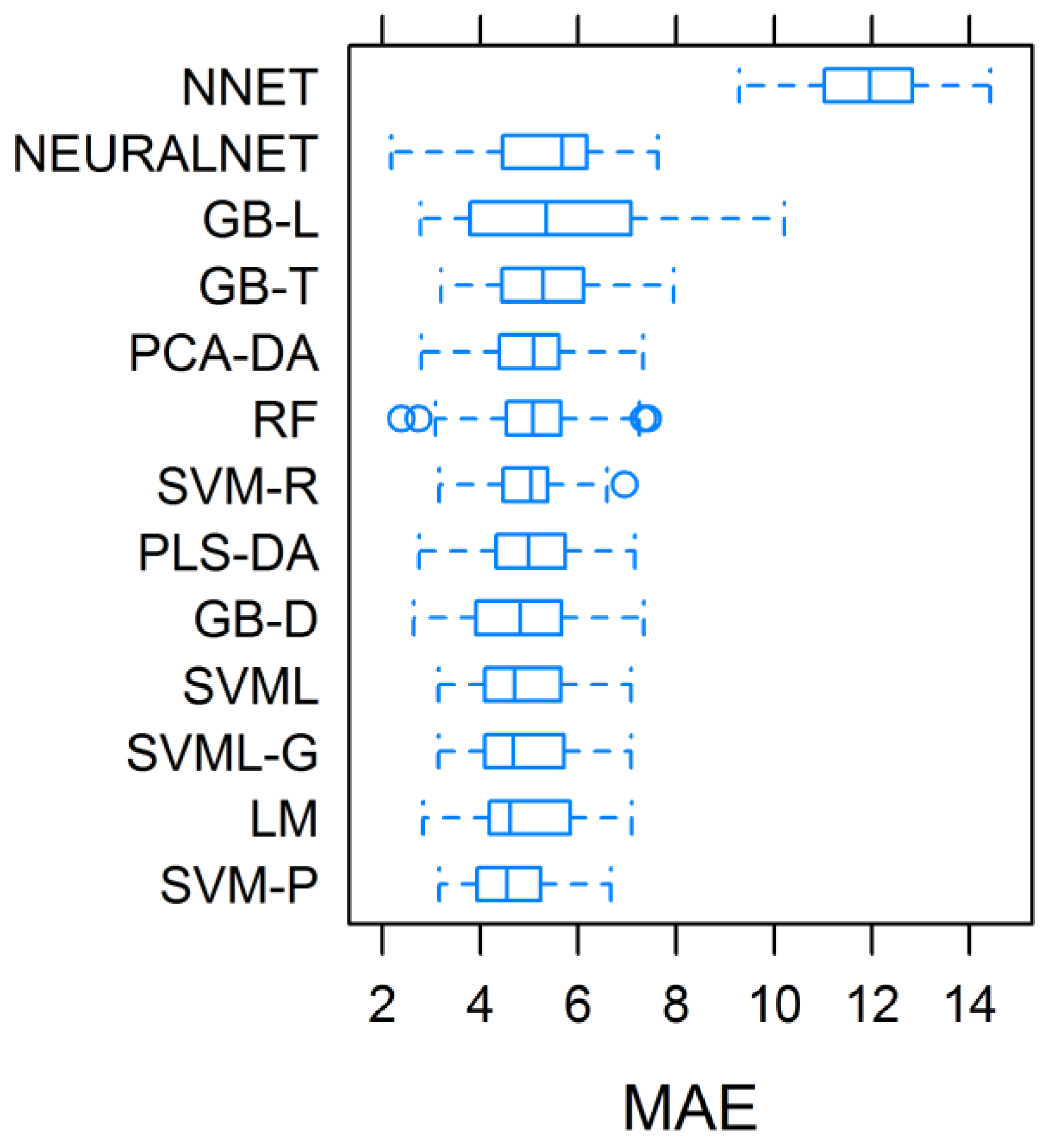
3.2. Assessment and Validation of the Predictive Models, and Importance of Regressors in Total Biomass Prediction

Thirteen models implemented in this work were assessed using the prediction accuracy (Table 2) in the validation set, the mean absolute error (MAE) and mean absolute percentage error (MAPE) metrics (Table 2, Figure 4) produced during the repeated cross-validation, and during the validation stage in the independent sample set. A repeated cross-validation iteration was run for each model, resulting in MAE resample vectors, each containing 50 elements. Over the months evaluated, the range and mean accuracy (Table 2) for NNET, RF, SVM-R, PCA-DA, PLS-DA, SVM-P, SVML, SVML-G, GBT, GBD, GBL, LM, and NLNET, were 0.16–0.78 and 0.56, 0.39–0.82 and 0.63, −0.36–0.88 and 0.16, −0.13–0.76 and 0.43, −0.02–0.77 and 0.47, 0.09–0.81 and 0.50, 0.49–0.80 and 0.64, 0.46–0.80 and 0.64, 0.56–0.81 and 0.66, −0.01–0.84 and 0.49, 0.03–0.93 and 0.47, 0.46–0.78 and 0.61, and 0.01–0.79 and 0.47, respectively.
The mean comparison showed that SVM-R was the least accurate model. The other models showed comparable accuracies, but RF, SVML, SVML-G, SVM-P, NNET, GBT, and GBD showed prediction ability greater than SVM-R. GBT’s prediction ability was consistently greater than 0.5 across the prediction times. Apart from GBL, the prediction ability of all models was high (prediction accuracy greater than or equal to 0.76) and/or better in the month of May (Table 2). The mean accuracy across models was high and not significantly different in May, May–June, and May–July. The across-model average accuracy computed in May was significantly superior to the mean accuracy obtained in June, June–July, and July. June, June–July, and July were statistically equally worst times for predicting biomass yields in sorghum under the Mediterranean region.
The range and mean MAE values (in t ha−1) produced for each model during the calibration experiments at one (May) of the best prediction times were 9.3–14.4 and 12.0, 2.4–7.4 and 5.0, 3.1–7.0 and 4.9, 2.8–7.3 and 5.0, 2.7–7.2 and 5.0, 3.1–6.7 and 4.6, 3.1–7.1 and 4.8, 3.1–7.1 and 4.8, 3.19–7.95 and 5.29, 2.64–7.34 and 4.80, 2.77–10.21 and 5.43, 2.82–7.09 and 4.88, and 2.18–7.63 and 5.36, for NNET, RF, SVM-R, PCA-DA, PLS-DA, SVM-P, SVML, SVM-G, GBT, GBD, GBL, LM, and NLNET, respectively (Figure 4, Table 2). The average MAE values during the training process were statistically higher in NNET followed by NLNET and GBL. Prediction error (MAE) was lower in SVM-P and GBD, while it was not statistically different in PLS-DA, PCA-DA, RF, SVML, SVML-G, SVM-R, GBT, and LM (Figure 4, Table 2). The MAE values (in t ha−1) calculated using the validation (testing) set and the best prediction time (May) were, in increasing order, 1.87 (13.85%), 2.18 (16.15%), 2.27 (16.81%), 2.34 (17.33%), 2.68 (19.85%), 2.91 (21.56%), 3.40 (25.19%), 3.62 (26.81%), 3.74 (27.70%), 3.74 (27.7%), 4.53 (33.56%), 6.22 (46.07%), and 12.5 (92.59%), for SVM-R, GBD, RF, NLNET, GBT, PCA-DA, GBL, PLS-DA, SVML, SVML-G, LM, SVM-P, and NNET algorithms, respectively.
Spearman’s rank correlation coefficient (Spearman’s rho) between model accuracy and MAE values (t ha−1 and %) corresponding to the testing set was −0.40. The Spearman’s rho method assesses how well the relationship between two variables can be described using a monotonic function between ordered sets that preserves or reverses the given order [48]. The Spearman’s rho approach was selected to account for the small size of the samples whose pairwise statistical dependences could not be correctly assessed with parametric approaches that have to be implemented on normally distributed data. Indeed the Shapiro–Wilk test of normality for the vectors of model accuracies and MAE values, was very highly significant (p < 0.001), meaning that we couldn’t assume the normality.
Over the May to July prediction time interval, six days of year corresponding to fortnightly fAPAR indices, were used as regressors in this work. Among these regressors, the most important times to predict the aboveground sorghum biomass yields were investigated using the GBT algorithm as this model showed high and dependable performance that was insensitive to the prediction times across the cropping season. The model showed that the day of year 150 was the most important (index = 100) followed by DoY 165 (index = 80), DoY 135 (index = 30), DoY 195 (index = 20), and DoY 210 (index = 10) (Figure 5). The day of year 180 was associated with no importance in terms of fAPAR-based prediction of the aboveground biomass yields in sorghum under the Mediterranean environment.

4. Discussion

The fAPAR biophysical variable used in this work was derived from satellite imagery, which is part of Earth Observation’s big data. Big data technology (BDT) is a new technological paradigm that is driving entire economies, including low-tech industries such as agriculture where it is implemented under the banner of precision farming (PF) [49]. In this work, BDT was built on geocoded maps of agricultural experiment fields and the real-time monitoring of sorghum crops on commercial farms in order to assess the possibility to monitor sorghum growth and development, with the ultimate aim of predicting the aboveground biomass yields. Early prediction of biomass production has positive implications including increased efficiency in biomass, biofuel, and farming resource management [50], and avoidance of energy crises. Forty-two sorghum pilot trials were evaluated in this work using fAPAR and different sorghum varieties belonging to four biomass producing sorghum types of dual purpose, sweet, forage, and biomass per se. Combining different types of biomass producing sorghums in this study was motivated by the need to mimic farming practice in the Mediterranean region. In this region, farmers, farming cooperatives, and third-party biomass harvesting and biodigesting companies manage the above-mentioned sorghum types indiscriminately on a regular basis. It made therefore sense not to discriminate the biomass producing sorghum types as sources of variation in the models implemented in this work. Similar investigations were reported in previous studies working on different crop species [16,51]. Important regressors of interest were identified and used in the predictive algorithms as suggested in literature [14,51].
The fAPAR index produced unique curves and maps that discriminated between the types of sorghums evaluated in this work. The fAPAR profile paralleled the evolution of leaf senescence across sorghum types [52] under the Mediterranean environment. The fAPAR curves presented in this work were purposely derived from sorghum fields established side by side in the same location in Anzola dell’Emilia. These pilots were sown and harvested on the same dates and managed identically, which allows a coherent comparison. The above-described shapes of the curves were generally similar also across locations in this study, though with slight discrepancies for some sorghum types. All sorghum trials reported in this work were conducted under a rainfed regime. Given that Mediterranean region is characterized by a semiarid climate wherein summer crops rely heavily on winter soil-stored moisture and experience postanthesis drought stress, it can be inferred that the fAPAR in dual purpose and biomass sorghum types did not rise during the reproduction growth stage probably due to a combined effect of sink demand and soil water scarcity in dual purpose, and mostly soil water scarcity in biomass sorghum. Postanthesis drought stress in sorghum under the Mediterranean environment was amply described by Habyarimana et al. [52,53,54,55]. The fAPAR profile in the sweet, forage, and SB × SH grown from seed reflects the reduced importance of the sink and the delayed leaf senescence in these types. In these sorghum types, a slow fAPAR increase toward the harvest can be explained by the precipitations registered in early fall in most locations (Figures S1 and S2), which stimulated the growth of axillary tillers in annual Sorghum bicolor [54,55] and the growth of axillary tillers and ramets in perennial SB × SH sorghum [54,55,56,57]. The above explanation holds also in the case of the SB × SH regrown from rhizomes. In these plants, the deep fAPAR drop from mid-June (anthesis) to early fall corresponds to the observed dry summers (Figures S1 and S2) and testifies to the increased susceptibility to drought stress in these plants. The conclusions drawn on fAPAR profile held particularly for fields established in the same location. Therefore, further investigations with replications in time and space are in order before any generalization is made.
In this work, high levels of model prediction accuracy ( r 0.70 or r 2   0.50) were obtained for 12 out of the 13 models deployed at the best prediction time (May). The models were therefore able to explain 50% of the variability that existed in the sorghum biomass yield data, while the remaining variance can be related to other factors non accounted for in this study such as the heterogeneity of external environmental and anthropogenic factors including rainfall distribution, soil types, and planting/tilling practices that could lead to different yield responses across the farms. The modeling performance metrics achieved in this work are nonetheless comparable to previous findings. For instance, Battude et al. [58], Shafian et al. [31], and Panda et al. [30] came across similar accuracy in their work on maize biomass and grain yields, and sorghum yields, respectively. On the other hand, the accuracy realized in this work was greater or equal to the values reported in Gao et al. [51], Diouf et al. [14], and the optimal values in sorghum as presented in Johnson [16]. Linear and nonlinear models performed comparably in terms of accuracy and mean absolute error implying that the relationship between fAPAR and biomass yield was mainly linear, which was expected and also supported by previous findings [14]. At the best prediction time (month of May), the correlation between the model accuracies and the MAE values was negative, denoting the expected inverse relationship between the two metrics of model prediction performance.
The simple linear model was implemented in this work to serve as a benchmark with respect to the most complex models requiring parameters optimization. Since thirteen models were implemented in this study, it is interesting to select the best algorithms. As biomass sorghum in the Mediterranean region is harvested from end of August to late November, it can be interesting to be able to predict the biomass production from May to July, allowing the farmer to know the amount to be produced one to six months ahead of harvest [42,51]. SVML, SVML-G, GBT, and LM showed good prediction accuracy ( r 0.50 ) across the evaluated prediction times, with MAE values (%) of 27.70, 27.70, 19.85, and 33.56, respectively. The GBT model was therefore the best algorithm as it performed consistently well ( r 0.60 ) across the prediction times, and was associated with low prediction error. The GBT model can therefore be recommended for sorghum biomass yield prediction using Sentinel-2-derived fAPAR as biophysical variable under the Mediterranean region. This model can be deployed anywhere from May to July without significant loss function.
In terms of biomass yields prediction times, June, July, and June–July were the worst times. May, May–June, and May–July showed comparable average accuracies, but accuracy in May was generally high ( r 0.70 ) across models except GBL. The month of May can therefore be recommended as the best time to predict sorghum biomass yields in the Mediterranean region. In this work, several types of sorghum were used, including high tonnage, sweet, forage, and dual purpose types. The suitability of the month of May for sorghum biomass yields prediction can be partly explained by the fact that in early sorghum growth stages, particularly in the period of time around the fast growth stage, the four sorghum types exhibit similar levels of growth and development. Furthermore, sorghum crop as currently grown in the Mediterranean region, reaches the fast growth stage generally in the month of May, meaning that predictions run in May are carried out on populations of sorghum types that are mostly at the same stage of growth and development. Overall, the days of year 150 and 165 were the most important regressors followed by days of year 135, 195, and 210 in decreasing order. The two regressors acquired in May (DoY 150 and 135) had important direct effects on the sorghum biomass, which justifies the good prediction accuracies obtained in this month. On the other hand, the two regressors corresponding to the month of July showed poor importance on biomass yields, while one of the two regressors corresponding to the month of June had meaningless effect on biomass yields, all of which explains the poor prediction accuracies obtained in June, July, and June–July (Table 2). In the Mediterranean region, sorghum is sown mid-to-late April. Therefore, being able to perform accurate sorghum biomass yields prediction in May, i.e., up to six months ahead of harvesting is a remarkable opportunity for the farmer and farming cooperatives that can use this information for several business-related purposes. They can efficiently organize the biomass business operations including the rational mobilization of the fleets of harvesting machinery, transport vehicles, and storage facilities. The predictive models developed in this work can also be used by extension services and policy-makers for strategic purposes. Obtaining the information on potential within-season biomass availability early on before actual harvest will help assess alternative means for energy supply internally, import or export, which is expected to help avoid specific crises such as fuel shortage. The findings in this work are limited in scope to one province in Italy, within the Mediterranean region. The prediction equations produced in this work can therefore be safely used in analogous modeling experiments in other Mediterranean areas. However, for these equations to be extended to modeling activity at a global level, the training populations of farms would require updates with inclusion of data accounting for sampling additional latitudes and longitudes relevant for sorghum cultivation.

5. Conclusions

The importance of sorghum as food, feed, and biofuel crop was amply described in several scientific literatures. Biomass sorghum demonstrated higher yields with better energy balance relative to major crops of agroindustrial interest. As dedicated biomass sorghum crops are steadily increasing and precision farming is driving agricultural economies worldwide, the harnessing satellite technology is well-poised to bring about agricultural advantages including cutting farming operational costs. Sentinel-2-derived fraction of absorbed photosynthetically active radiation was found to satisfactorily explain primary productivity and was used in this study as biophysical variable in the predictive modeling of aboveground biomass yields in annual and perennial sorghums. Across month combinations from May to July and the thirteen machine learning prediction algorithms used in this work, the gradient boosting machine learning algorithm implementing xgbtree was identified as the best predictive model. The best prediction time for sorghum biomass was particularly the month of May, followed by May–June and May–July using fortnightly fAPAR indices. To the best of our knowledge, the present work represents the first time Sentinel-2-derived fAPAR is used in predictive modeling of sorghum biomass yields. The outcome from this study is important and can serve several purposes including farmers being able to improve their sorghum biomass business operations. Policy-makers and extension services will also benefit from the findings in this work allowing them early on within season information on potential biomass availability, which is critical to wider energy planning and avoiding energy-related crises.

Supplementary Materials

The following are available online at https://www.mdpi.com/2073-4395/9/4/203/s1, Figure S1: Fifteen-day averaged temperatures and rainfall in Anzola dell’Emilia in 2017 and 2018 cropping seasons, Figure S2: Fifteen-day averaged temperatures and rainfall in Conselice in 2017 and 2018 cropping seasons, Figure S3: Fifteen-day averaged temperatures and rainfall in Mirandola in 2017 and 2018 cropping seasons, Figure S4: Fifteen-day averaged temperatures and rainfall in Nonantola in 2017 cropping season.

Author Contributions

Conceptualization, E.H.; Data Curation, E.H. and I.P.; Formal Analysis, E.H.; Funding Acquisition, E.H. and I.P.; Investigation, E.H.; Methodology, E.H.; Project Administration, E.H.; Writing—Original Draft, E.H.; Writing—Review & Editing, I.P., M.C., P.D.F., and M.D.

Acknowledgments

Part of this work was supported (beneficiary: first author) by the project Data-driven Bioeconomy (www.databio.eu), GA number: 732064 (H2020-ICT-2016-1—innovation action), and the project Risorse GeneticheVegetali (RGV/FAO) 2014e2016 of the Ministero delle PoliticheAgricole, Alimentari e Forestali, Rome. The authors would like to thank the anonymous reviewers and editor for their informative remarks that contributed to improving the quality of this paper.

Conflicts of Interest

The authors declare no conflicts of interest.

References

  1. Habyarimana, E.; Lorenzoni, C.; Redaelli, R.; Alfieri, M.; Amaducci, S.; Cox, S. Towards a perennial biomass sorghum crop: A comparative investigation of biomass yields and overwintering of Sorghum bicolor x S. halepense lines relative to long term S. bicolor trials in northern Italy. Biomass Bioenergy 2018, 111, 187–195. [Google Scholar] [CrossRef]
  2. Damasceno, C.M.B.; Schaffert, R.E.; Duweikat, I. Mining Genetic Diversity of Sorghum as a Bioenergy Feedstock; Springer: New York, NY, USA, 2014; pp. 81–106. [Google Scholar]
  3. Hoffmann, L., Jr.; Rooney, W.L. Cytoplasm has no effect on the yield and quality of biomass sorghum hybrids. JSBS 2013, 3, 129–134. [Google Scholar] [CrossRef]
  4. Prakasham, R.S.; Nagaiah, D.; Vinutha, K.S.; Uma, A.; Chiranjeevi, T.; Umakanth, A.V. Sorghum biomass: A novel renewable carbon source for industrial bioproducts. Biofuels 2014, 5, 159–174. [Google Scholar] [CrossRef]
  5. Habyarimana, E. Genomic prediction for yield improvement and safeguarding of genetic diversity in CIMMYT spring wheat (Triticum aestivum L.). Aust. J. Crop Sci. 2016, 10, 127–136. [Google Scholar]
  6. Rooney, W.L. Genetics and cytogenetics. In Sorghum: Origin, History, Technology, and Production; Smith, C.W., Frederiksen, R.A., Eds.; John Wiley & Sons: New York, NY, USA, 2000; pp. 261–307. [Google Scholar]
  7. El Bassam, N. Handbook of Bioenergy Crops: A Complete Reference to Species, Development and Applications; Earthscan Ltd.: London, UK, 2010; pp. 45–477. [Google Scholar]
  8. Stefaniak, T.R.; Dahlberg, J.A.; Bean, B.W.; Dighe, N.; Wolfrum, E.J.; Rooney, W.L. Variation in biomass composition components among forage, biomass, sorghum-sudangrass, and sweet sorghum types. Crop Sci. 2012, 52, 1949–1954. [Google Scholar] [CrossRef]
  9. Kussul, N.; Sokolov, B.V.; Zyelyk, Y.I.; Zelentsov, V.A.; Skakun, S.V.; Shelestov, A.Y. Disaster risk assessment based on heterogeneous geospatial information. J. Autom. Inform. Sci. 2010, 42, 32–45. [Google Scholar] [CrossRef]
  10. Kussul, N.; Shelestov, A.; Skakun, S. Flood Monitoring from SAR Data Use of Satellite and In-Situ Data to Improve Sustainability; Springer: Dordrecht, The Netherlands, 2011; pp. 19–29. [Google Scholar]
  11. Skakun, S.; Kussul, N.; Kussul, O.; Shelestov, A. Quantitative estimation of drought risk in Ukraine using satellite data. In Proceedings of the IEEE International Geoscience and Remote Sensing Symposium (IGARSS), Quebec City, QC, Canada, 13–18 July 2014; pp. 5091–5094. [Google Scholar]
  12. Skakun, S.; Kussul, N.; Shelestov, A.; Kussul, O. The use of satellite data for agriculture drought risk quantification in Ukraine. Geomat. Nat. Hazards Risk 2016, 7, 901–917. [Google Scholar] [CrossRef]
  13. Gallego, J.; Kravchenko, A.N.; Kussul, N.N.; Skakun, S.V.; Shelestov, A.Y.; Grypych, Y.A. Efficiency assessment of different approaches to crop classification based on satellite and ground observations. J. Autom. Inform. Sci. 2012, 44, 67–80. [Google Scholar] [CrossRef]
  14. Diouf, A.A.; Brandt, M.; Verger, A.; El Jarroudi, M.; Djaby, B.; Fensholt, R.; Ndione, J.A.; Tychon, B. Fodder Biomass Monitoring in Sahelian Rangelands Using Phenological Metrics from FAPAR time series. Remote Sens. 2015, 7, 9122–9148. [Google Scholar] [CrossRef]
  15. Duveiller, G.; López-Lozano, R.; Baruth, B. Enhanced Processing of 1-km Spatial Resolution fAPAR Time Series for Sugarcane Yield Forecasting and Monitoring. Remote Sens. 2013, 5, 1091–1116. [Google Scholar] [CrossRef] [Green Version]
  16. Johnson, D.M. A comprehensive assessment of the correlations between field crop yields and commonly used MODIS products. Int. J. Appl. Earth Obs. Geoinf. 2016, 52, 65–81. [Google Scholar] [CrossRef] [Green Version]
  17. Kogan, F.; Kussul, N.; Adamenko, T.; Skakun, S.; Kravchenko, O.; Kryvobok, O.; Shelestov, A.; Kolotii, A.; Kussul, O.; Lavrenyuk, A. Winter wheat yield forecasting in Ukraine based on Earth observation, meteorological data and biophysical models. Int. J. Appl. Earth Obs. Geoinf. 2013, 23, 192–203. [Google Scholar] [CrossRef]
  18. Kogan, F.; Kussul, N.; Adamenko, T.; Skakun, S.; Kravchenko, O.; Kryvobok, O.; Shelestov, A.; Kolotii, A.; Kussul, O.; Lavrenyuk, A. Winter wheat yield forecasting: A comparative analysis of results of regression and biophysical models. Int. J. Autom. Inform. Sci. 2013, 45, 68–81. [Google Scholar] [CrossRef]
  19. Kowalik, W.; Dabrowska-Zielinska, K.; Meroni, M.; Raczka, T.U.; de Wit, A. Yield estimation using SPOTVEGETATION products: A case study of wheat in European countries. Int. J. Autom. Inform. Sci. 2014, 32, 228–239. [Google Scholar]
  20. Kross, A.; McNairn, H.; Lapen, D.; Sunohara, M.; Champagne, C. Assessment of RapidEye vegetation indices for estimation of leaf areaindex and biomass in corn and soybean crops. Int. J. Appl. Earth Obs. Geoinf. 2015, 34, 235–248. [Google Scholar] [CrossRef]
  21. Camacho, F.; Cernicharo, J.; Lacaze, R.; Baret, F.; Weiss, M. GEOV1: LAI, FAPAR Essential Climate Variables and FCOVER global time series capitalizing over existing products. Part 2: Validation and intercomparison with reference products. Remote Sens. Environ. 2013, 137, 310–329. [Google Scholar] [CrossRef]
  22. Shelestov, A.; Kolotii, A.; Camacho, F.; Skakun, S.; Kussul, O.; Lavrenuik, M. Mapping of biophysical parameters based on high resolution EO imagery for JECAM test site in Ukraine. In Proceedings of the 2015 IEEE International Geoscience and Remote Sensing Symposium (IGARSS), Milan, Italy, 26–31 July 2015. [Google Scholar]
  23. Kussul, N.; Kolotii, A.; Skakun, S.; Shelestov, A.; Kussul, O.; Oliynuk, T. Efficiency estimation of different satellite data usage for winter wheat yield forecasting in Ukraine. In Proceedings of the 2014 IEEE International Geoscience and Remote Sensing Symposium (IGARSS), Quebec City, QC, Canada, 13–18 July 2014; pp. 5080–5082. [Google Scholar]
  24. López-Lozano, R.; Duveiller, G.; Seguini, L.; Meroni, M.; García-Condado, S.; Hooker, J.; Leo, O.; Baruth, B. Towards regional grain yield forecasting with 1km-resolution EO biophysical products: Strengths and limitations at pan-European level. Agric. For. Meteorol. 2015, 206, 12–32. [Google Scholar] [CrossRef] [Green Version]
  25. Baret, F.; Weiss, M.; Lacaze, R.; Camacho, F.; Makhmara, H.; Pacholcyzk, P.; Smets, B. Geov1: LAI and FAPAR essential climate variables and FCOVER global time series capitalizing over existing products. Part1: Principles of development and production. Remote Sens. Environ. 2013, 137, 299–309. [Google Scholar] [CrossRef]
  26. Fensholt, R.; Sandholt, I.; Rasmussen, M.S.; Stisen, S.; Diouf, A. Evaluation of satellite based primary production modelling in the semi-arid Sahel. Remote Sens. Environ. 2006, 105, 173–188. [Google Scholar] [CrossRef]
  27. Tucker, C.J.; Holben, B.N.; Elgin, J.H.; McMurtrey, J.E. Relationship of spectral data to grain yield variation. Photogramm. Eng. Remote Sens. 1980, 46, 657–666. [Google Scholar]
  28. Barnett, T.L.; Thompson, D.R. The use of large-area spectral data in wheatyield estimation. Remote Sens. Environ. 1982, 12, 509–518. [Google Scholar] [CrossRef]
  29. Hatfield, J.L. Remote sensing estimators of potential and actual crop yield. Remote Sens. Environ. 1996, 13, 301–311. [Google Scholar] [CrossRef]
  30. Panda, S.S.; Ames, D.P.; Panigrahi, S. Application of vegetation indices for agricultural crop yield prediction using neural network techniques. Remote Sens. 2010, 2, 673–696. [Google Scholar] [CrossRef]
  31. Shafian, S.; Rajan, N.; Schnell, R.; Bagavathiannan, M.; Valasek, J.; Shi, Y.; Olsenholler, J. Unmanned aerial systems-based remote sensing for monitoring sorghum growth and development. PLoS ONE 2018, 13, e0196605. [Google Scholar] [CrossRef] [PubMed]
  32. Yang, C.; Everitt, J.H.; Bradford, J.M.; Escobar, D.E. Mapping grain sorghum growth and yield variations using airborne multispectral digital imagery. Trans. ASAE 2000, 43, 1927–1938. [Google Scholar] [CrossRef]
  33. Piper, J.K.; Kulakow, P.A. Seed yield and biomass allocation in Sorghum bicolor and F1 and backcross generations of S. bicolor x S. halepense hybrids. Can. J. Bot. 1994, 72, 468–474. [Google Scholar] [CrossRef]
  34. De Keukelaere, L.; Sterckx, S.; Adriaensen, S.; Knaeps, E.; Reusen, I.; Giardino, C.; Bresciani, M.; Hunter, P.; Neil, C.; Van der Zande, D.; et al. Atmospheric correction of Landsat-8/OLI and Sentinel-2/MSI data using iCOR algorithm: Validation for coastal and inland waters. Eur. J. Remote Sens. 2018, 51, 525–542. [Google Scholar] [CrossRef]
  35. Weiss, M.; Baret, F. ATBD S2ToolBox Level 2 Products: LAI, FAPAR, FCOVER (Version 1.1). 2016. Available online: http://step.esa.int/docs/extra/ATBD_S2ToolBox_L2B_V1.1.pdf (accessed on 7 November 2018).
  36. Jacquemoud, S.; Verhoef, W.; Baret, F.; Bacour, C.; Zarco-Tejada, P.J.; Asner, G.P.; François, C.; Ustin, S.L. PROSPECT + SAIL models: A review of use for vegetation characterization. Remote Sens. Environ. 2009, 113, S56–S66. [Google Scholar] [CrossRef]
  37. Sage, R.F. A portrait of the C4 photosynthetic family on the 50th anniversary of its discovery: Species number, evolutionary lineages, and Hall of Fame. J. Exp. Bot. 2016, 67, 4039–4056. [Google Scholar] [CrossRef]
  38. Eilers, P.H.C. A perfect smoother. Anal. Chem. 2003, 75, 3631–3636. [Google Scholar] [CrossRef]
  39. Atzberger, C.; Eilers, P.H.C. A smoothed 1-km resolution NDVI time series (1998–2008) for vegetation studies in South America. Int. J. Digit. Earth 2010, 4, 365–386. [Google Scholar] [CrossRef]
  40. Kuhn, M. Building predictive models in R using the caret Package. J. Stat. Softw. 2008, 28, 1–26. [Google Scholar] [CrossRef]
  41. Benor, D.; Baxter, M. Training and Visit Extension; The World Bank: Washington, DC, USA, 1984; pp. 21–212. [Google Scholar]
  42. Hoefsloot, P.; Ines, A.V.; van Dam, J.; Duveiller, G.; Kayitakire, F.; Hansen, J. Combining crop models and remote sensing for yield prediction: Concepts, applications and challenges for heterogeneous smallholder environments. In JRC Scientific and Policy Reports; Report of CCFAS-JRC Workshop at Joint Research Centre; Joint Research Centre of the European Commission: Ispra, VA, Italy, 2012; pp. 7–41. [Google Scholar]
  43. Meuwissen, T.H.E.; Hayes, B.J.; Goddard, M.E. Prediction of total genetic value using genome-wide dense marker maps. Genetics 2001, 157, 1819–1829. [Google Scholar] [PubMed]
  44. R Core Team. R: A Language and Environment for Statistical Computing; R Foundation for Statistical Computing: Vienna, Austria, 2013. [Google Scholar]
  45. Breiman, L.; Friedman, J.H.; Olshen, R.A.; Stone, C.J. Classification and Regression Trees; Wadsworth Inc.: Blelmont, CA, USA, 1984. [Google Scholar]
  46. Willmott, C.J.; Matsuura, K. Advantages of the mean absolute error (MAE) over the root mean square error (RMSE) in assessing average model performance. Clim. Res. 2005, 30, 79–82. [Google Scholar] [CrossRef] [Green Version]
  47. Duncan, D.B. Multiple range and multiple F tests. Biometrics 1955, 11, 1–42. [Google Scholar] [CrossRef]
  48. Spearman, C. The proof and measurement of association between two things. Am. J. Psychol. 1904, 15, 72–101. [Google Scholar] [CrossRef]
  49. Schellberg, J.; Hill, M.J.; Gerhards, R.; Rothmund, M.; Braun, M. Precision agriculture on grassland: Applications, perspectives and constraints. Eur. J. Agron. 2008, 29, 59–71. [Google Scholar] [CrossRef]
  50. Segarra, E. Precision Agriculture Initiative for Texas High Plains; Annual Comprehensive Report; Texas A&M University Research and Extension Center: Lubbock, TX, USA, 2002. [Google Scholar]
  51. Gao, F.; Anderson, M.; Daughtry, C.; Johnson, D. Assessing the Variability of Corn and Soybean Yields in Central Iowa Using High Spatiotemporal Resolution Multi-Satellite Imagery. Remote Sens. 2018, 10, 1489. [Google Scholar] [CrossRef]
  52. Habyarimana, E.; Lorenzoni, C.; Busconi, M. Search for new stay-green sources in Sorghum bicolor (L.) Moench. Maydica 2010, 55, 187–194. [Google Scholar]
  53. Habyarimana, E.; Laureti, D.; Di Fonzo, N.; Lorenzoni, C. Biomass production and drought resistance at the seedling stage and in field conditions in sorghum. Maydica 2002, 47, 303–309. [Google Scholar]
  54. Habyarimana, E.; Laureti, D.; De Ninno, M.; Lorenzoni, C. Performances of biomass sorghum [Sorghum bicolor (L.) Moench] under different water regimes in Mediterranean region. Ind. Crop Prod. 2004, 20, 23–28. [Google Scholar] [CrossRef]
  55. Habyarimana, E.; Bonardi, P.; Laureti, D.; Di Bari, V.; Cosentino, S.; Lorenzoni, C. Multilocational evaluation of biomass sorghum hybrids under two stand densities and variable water supply in Italy. Ind. Crop Prod. 2004, 20, 3–9. [Google Scholar] [CrossRef]
  56. Cox, T.S.; Van Tassel, D.L.; Cox, C.M.; DeHaan, L.R. Progress in breeding perennial grains. Crop. Pasture Sci. 2010, 61, 513–521. [Google Scholar] [CrossRef]
  57. Nabukalu, P.; Cox, T.S. Response to selection in the initial stages of a perennial sorghum breeding program. Euphytica 2016, 209, 103–111. [Google Scholar] [CrossRef]
  58. Battude, M.; Al Bitar, A.; Morin, D.; Cros, J.; Huc, M.; Sicre, C.M.; Le Dante, V.; Demarez, V. Estimating maize biomass and yield over large areas using high spatial and temporal resolution Sentinel-2 like remote sensing data. Remote Sens. Environ. 2016, 184, 668–681. [Google Scholar] [CrossRef]
Figure 1. Map of Italy (A) with a rectangle inset indicating the geographical location of the experimental sites (red dots) for pilots established in 2017 (B) and 2018 (C).
Agronomy 09 00203 g001
Figure 2. Greenness (fAPAR) maps derived from Sentinel-2 satellite imagery for five sorghum fields in Anzola (from left to right: T5-grain sorghum, T4-dual purpose sorghum, T3-sweet sorghum, T2-forage sorghum, T1-biomass sorghum) for a selected number of dates in 2017, as available via WatchITgrow. T5-grain sorghum was not included in this study (refer to Section 2.1 for detail).
Agronomy 09 00203 g002
Figure 3. Greenness (fAPAR) graphs derived from Sentinel-2 satellite imagery from 2017 for six sorghum fields in Anzola (T4-dual purpose sorghum, T3-sweet sorghum, T2-forage sorghum, T1-biomass sorghum, and 16R17-perennial, 17US_mat perennial), available via WatchITgrow.
Agronomy 09 00203 g003aAgronomy 09 00203 g003b
Figure 4. Visualization of models MAE (t ha−1) dispersion using boxplot approach and fAPAR acquired in May. PLS-DA, PCA-DA, RF, SVML, SVML-G, SVM-R, SVM-P, NNET, GBT, GBD, GBL, LM, and NLNET, respectively, partial least squares discriminant analysis, principal component analysis discriminant analysis, random forest, Support Vector Machines with Linear Kernel, Support Vector Machines with Linear Kernel grid search, Support Vector Machines with Radial Basis Function Kernel, Support Vector Machines with Polynomial Kernel, neural network, eXtreme Gradient Boosting xgbtree method, eXtreme Gradient Boosting xgbDART method, eXtreme Gradient Boosting xgbLinear method, Linear model, and Neural Network neuralnet method.
Agronomy 09 00203 g004
Figure 5. Relative importance of regressors (day of year, D) on sorghum biomass yields in 2017 and 2018, using eXtreme Gradient Boosting xgbtree (GBT) method.
Agronomy 09 00203 g005
Table 1. Pilots descriptors: name, location, variety, season, and productivity.
Serial
Number
Field/Pilot
Name
Variety
Name
Variety
Type
Area (ha)Dry Biomass
Yield (t ha−1)
Cropping
Season
Location
Name
1Botte 1Harmattan Dual purpose9.0014.132018Conselice
2Saracca 5Harmattan Dual purpose6.5010.522018Conselice
3V. serrataHarmattan Dual purpose44.879.692018Conselice
4MagnanaP845FForage32.0511.432018Conselice
5Cà biancaP845FForage3.7211.112018Conselice
6Gamberina 3Aralba Dual purpose7.869.672018Conselice
7SagrateHarmattanDual purpose50.008.902017Conselice
8Prato_MensaHarmattanDual purpose3.2919.102017Conselice
9ComunaP845FForage27.8624.502017Conselice
10Gamberina_1AralbaDual purpose7.6012.802017Conselice
11BotteHarmattanDual purpose5.3323.502017Conselice
12Carafolo_GBulldozerBiomass2.0017.102017Nonantola
13Cavriani_SMerlin Biomass2.0019.502017Nonantola
14Ferrari_RBulldozerBiomass1.003.402017Nonantola
15Mattioli_RBulldozerBiomass1.004.902017Nonantola
16Serafini_GBulldozerBiomass2.0015.302017Nonantola
17Zavatti_EBulldozerBiomass0.897.602017Mirandola
18Grandi_MagonzaBulldozerBiomass0.8012.802017Mirandola
19Grandi_PonteBulldozerBiomass1.209.502017Mirandola
20Zini_L Palo AltoBiomass2.508.002017Mirandola
21Villa_verdettaBulldozerBiomass1.006.252018Mirandola
22Cama_grandeBulldozerBiomass4.4014.942018Mirandola
23Cama_piccoloBulldozerBiomass4.0015.352018Mirandola
24Golinelli_RaimondoBulldozerBiomass2.0210.482018Mirandola
25Barozzi_LidiaBulldozerBiomass3.007.192018Mirandola
26Molon_A Palo AltoBiomass5.008.302017Mirandola
27T1_AnzolaSoleBiomass0.7413.002017Anzola
28T2_AnzolaTrudanForage0.7119.002017Anzola
29T3_AnzolaHannibalSweet0.7117.002017Anzola
30T4_AnzolaHarmattanDual purpose0.7014.002017Anzola
31T1_AnzolaBulldozerBiomass0.7417.002018Anzola
32T2_AnzolaHannibalSweet0.7119.002018Anzola
33T3_AnzolaTarzanBiomass0.7121.002018Anzola
34T4_AnzolaTrudanForage0.7013.002018Anzola
35T5_AnzolaHarmattanDual purpose0.7015.002018Anzola
3615R17PerennialBiomass0.062.392017Anzola
3716R17PerennialBiomass0.158.272017Anzola
3817IT_matBicolorBiomass0.1718.302017Anzola
3917US_matBicolorBiomass0.1521.002017Anzola
4016R18PerennialBiomass0.1514.352018Anzola
4115R18PerennialBiomass0.0610.732018Anzola
4217R18PerennialBiomass0.1517.472018Anzola
Table 2. Predictive models × prediction time accuracies and May MAE for the training and validation sets.
(1) Model(2) Accuracy(3) May_MAE.T
t ha−1
May_MAE.V
MayJuneJulyMay–JuneJune–JulyMay–JulyMeant ha−1%
PLS-DA0.770.49−0.020.690.320.560.47 ab5.01 bcd3.6226.81
PCA-DA0.760.49−0.130.670.290.520.43 ab5.00 bcd2.9121.56
RF0.820.390.640.680.530.740.63 a5.05 bcd2.2716.81
SVML0.800.490.580.670.590.700.64 a4.82 cd3.7427.70
SVML-G0.800.490.580.660.610.720.64 a4.84 cd3.7427.70
SVM-R0.88−0.360.510.02−0.150.080.16 b4.95 bcd1.8713.85
SVM-P0.810.490.090.630.420.530.50 a4.64 d6.2246.07
NNET0.780.560.160.750.380.700.56 a11.99 a12.5092.59
GBT0.780.560.690.580.810.570.66 a5.29 bc2.6819.85
GBD0.840.37−0.010.760.480.510.49 a4.80 d2.1816.15
GBL0.450.110.890.930.030.430.47 ab5.43 b3.4025.19
LM0.780.500.560.730.460.650.61 ab4.88 cd4.5333.56
NLNET0.790.090.330.790.010.790.47 ab5.36 b2.3417.33
MEAN0.77a0.36b0.37b0.66a0.37b0.58ab0.525.544.0029.63
(1) PLS-DA, PCA-DA, RF, SVML, SVML-G, SVM-R, SVM-P, NNET, GBT, GBD, GBL, LM, and NLNET, respectively, partial least squares discriminant analysis, principal component analysis discriminant analysis, random forest, Support Vector Machines with Linear Kernel, Support Vector Machines with Linear Kernel grid search, Support Vector Machines with Radial Basis Function Kernel, Support Vector Machines with Polynomial Kernel, neural network, eXtreme Gradient Boosting- xgbtree method, eXtreme Gradient Boosting- xgbDART method, eXtreme Gradient Boosting-xgbLinear method, Linear model, and Neural Network neuralnet method. (2) Accuracy represents the Pearson correlation coefficient between the predicted and the observed values in the validation set. (3) May_MAE.T mean absolute error relative to the optimal prediction model in the month of May using repeated cross-validation in the training set; May MAE.V (MAE and MAPE) magnitude of the error relative to the predicted values in the validation (testing) set; means with the same letter in a same column or row, are not significantly different at the 5% probability level using Duncan’s multiple range test.

