Abstract
The landforms of the Earth’s surface ranging from large-scale features to local topography are factors that influence human behavior in terms of habitation practices. The ability to extract geomorphological settings using geoinformatic techniques is an important aspect of any environmental analysis and archaeological landscape approach. Morphological data derived from DEMs with high accuracies (e.g., LiDAR data), can provide valuable information related to landscape modelling and landform classification processes. This study applies the first landform classification and flood hazard vulnerability of 730 Eneolithic (ca. 5000–3500 BCE) settlement locations within the plateau-plain transition zone of NE Romania. The classification was done using the SD (standard deviation) of TPI (Topographic Position Index) for the mean elevation (DEV) around each archaeological site, and HEC-RAS flood hazard pattern generated for 0.1% (1000 year) discharge insurance. The results indicate that prehistoric communities preferred to place their settlements for defensive purposes on hilltops, or in the close proximity of a steep slope. Based on flood hazard pattern, 8.2% out of the total sites had been placed in highly vulnerable areas. The results indicate an eco-cultural niche connected with habitation practices and flood hazard perception during the Eneolithic period in the plateau-plain transition zone of NE Romania and contribute to archaeological predictive modelling.
1. Introduction
The ability to describe the geomorphological setting based on GIS-landform classification is an important aspect of any environmental analysis or landscape modelling effort [1,2]. Landforms are defined as specific geomorphic features on the Earth’s surface, ranging from large-scale features (e.g., plains, mountain ranges) to small-scale features (e.g., individual hills, valleys), as well as their component landforms, such as hilltops, valley bottoms, exposed ridges, flat plains, and upper or lower slopes [1,2,3]. In recent decades, the development of GIS software and free access to datasets has attracted the interest of researchers in implementing new computer algorithms to approach the morphometric attributes and topography of the Earth’s surface [2,4]. Also, there has been an upward trend in the use of GIS-based analysis to classify landforms over various scientific fields such as geo-pedology [5,6,7,8], geomorphology and seafloor mapping [9,10,11,12,13,14,15], hydrology [16,17,18], climatology [19], landscape mapping and ecology [20,21], and archaeology [4,22,23,24]. The morphological features provide useful information for archaeological studies because the data can be interlinked with settlement distribution [25], and evolution for reconstructing the paleo-landscapes [26,27]. In this context, one of the first approaches to find application in archaeological studies was the analysis of convexity, concavity, and flatness of the topographic surface [28,29,30,31]. Despite this, at present only a few studies with applications in the field of archaeology based on GIS-landform classifications have been developed [4,24,28,29]. In recent years, there have been intensive applications of LiDAR data in the analysis of floods in a GIS environment [32,33], yet no applications towards prehistoric flood hazards.
The territory of NE Romania is characterized by a high density of Eneolithic archaeological sites (chronological framework: ca. 5000–3500 BCE), which corresponds to the Precucuteni period (ca. 5000–4600 BCE) and Cucuteni-Trypillian culture (Cucuteni in Romania, ca. 4600–3500 BCE), known as the last great Eneolithic civilization of Old Europe [34,35,36,37,38]. In the Moldavian Plain (NE Romania), the Cucuteni culture is divided in Cucuteni A (ca. 4600–4100 BCE), Cucuteni A–B (ca. 4100–3850 BCE) and Cucuteni B (ca. 3850–3500 BCE) [35,39,40,41]. Besides the literature on the morphological features in the study area [42,43,44,45,46], only a few works deal with the local or the relative topographic position of archaeological settlements in the landscape [47,48]; most of them refer to the evaluation of cultural heritage sites to natural hazards (landslides, gully erosion) and anthropogenic impact [49,50,51,52,53,54].
Understanding the connections between the small-scale features, large-scale landforms, flood hazard perception, and the types of archaeological settlement is an important method applied in the study of the prehistoric peoples because the landscape can reveal insights into settlement distribution and dynamics over time [4,27]. This paper provides the first landform classification of 730 Eneolithic sites, using the TPI (Topographic Position Index) [3,5,28,55], and the SD (standard deviation) of the mean elevation, abbreviated as DEV by [29], around archaeological sites [3,4,29], which can classify the landscape in terms of slope position and landform categories and morphological classes based on the geomorphology [1,4,56,57]. The results can provide insights into factors favoring human habitation during the Eneolithic period in the plateau-plain transition zone of NE Romania and contribute to archaeological predictive modelling at regional-scale based on small-scale morphological features and flood hazard patterns [45,49,58,59,60,61].
Regional Setting
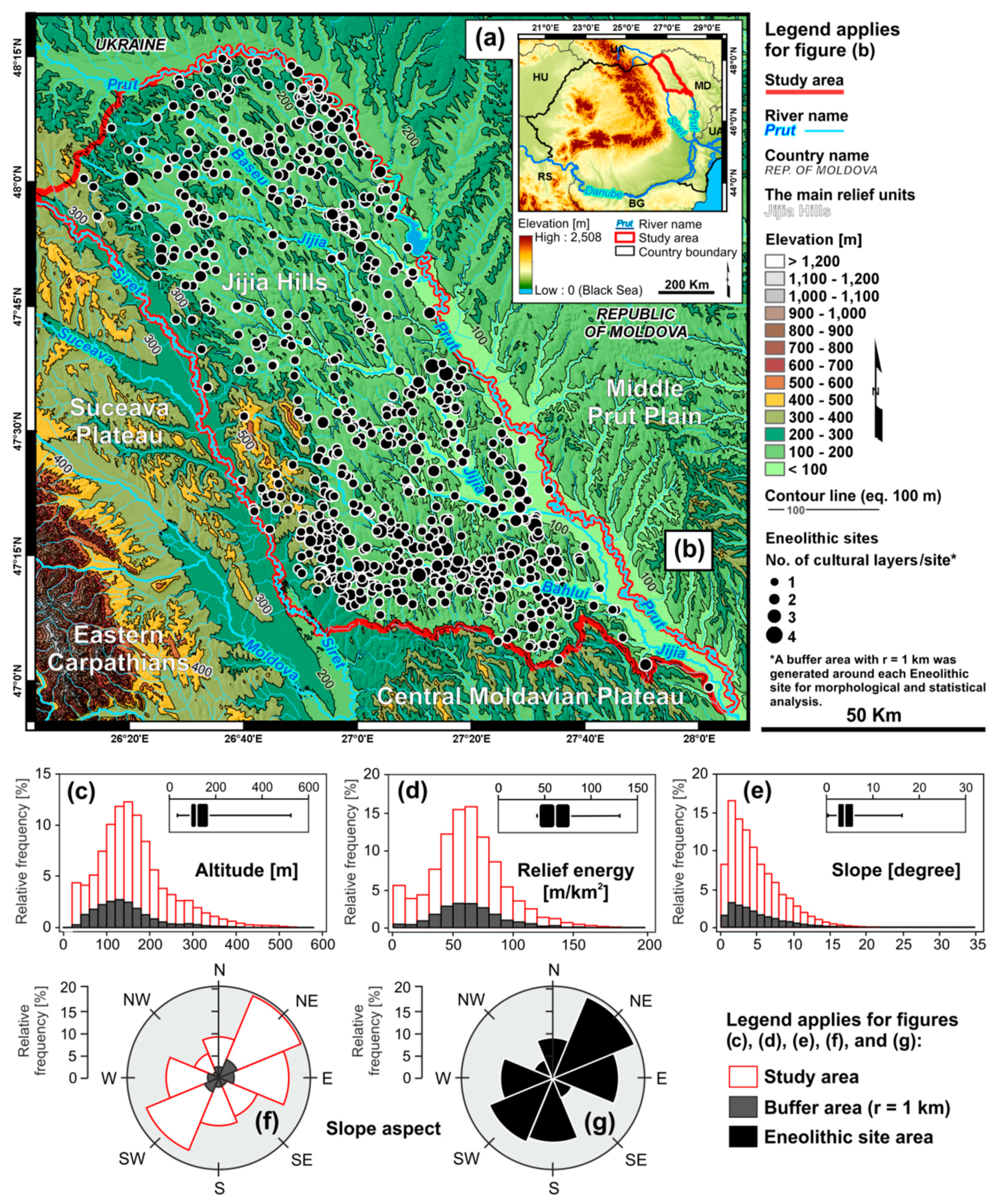
The study area (8789 km2) is located in the north-eastern part Romania, between the Siret floodplain in the west and the Prut floodplain in the north and east, where the Prut River is a natural border between Romania and the Republic of Moldova to the east and northeast, and Romania and Ukraine to the north [45,46] (Figure 1a). The southern limit is a structural one, represented by the contact area between the Moldavian Plain and the Central Moldavian Plateau [42]. The Moldavian Plain, known as the Jijia Plain, represents 88.65% (7880 km2) of the study area, and the Suceava Hills (Suceava Plateau) on the western flank, represent the remaining 11.35% (909 km2) (Figure 1b). The elevation range between 20 m a.s.l. and 591 m a.s.l., with an average of 163.5 m a.s.l. (Figure 1c). The relief energy does not exceed 150–200 m/km2, with an average of 63.4 m/km2, where the highest values indicate the contact area between plateau-plain transition zone and the smallest values indicate the floodplain of the Siret, Jijia and Prut rivers (Figure 1d). The slope average ranges between 0° and 38.88°, with an average value of 4.74° (Figure 1e). The highest declivity corresponds to the fronts of the cuestas, generally with an eastern or north-eastern slope aspect, and the gentle slope with the backs of the cuestas with southern or south-western aspects (Figure 1f,g).
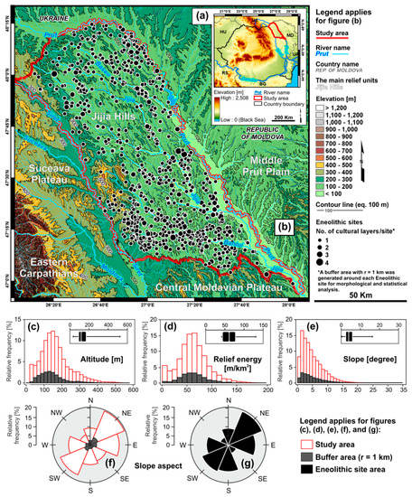
Figure 1.
(a) Geographic location of the study area in NE Romania; (b) the geoarchaeological context within Moldavian Plain; the distribution of (c) altitude, (d) relief energy, (e) slope angle, (f) and (g) slope aspect for study area, buffer area (r = 1 km) around each Eneolithic site, and for the settlement areas (intra-site).
The general morpho-structural setting consists of a monocline, dominated by cuesta landforms and deeply incised valleys, where the strata are gently dipping from northwest to southeast (Miocene-Pleistocene deposits) [42]. In the Suceava Hills (western flank) and the Moldavian Plain, the lithology is characterized by successions of clays with sands (200–300 m thick), and thin layers (2–30 m thick) of limestone and sandstone (Lower and Medium Sarmatian deposits) [42]. Over these, a loess layer lies over the entire study area, with thicknesses frequently less than 2 m [62], but which can reach a thickness of 15–30 m on the cuesta slopes and on fluvial terraces [48]. The gravel deposits occur in the alluvial plains of Siret and Prut rivers [45,46]. The landscape dominated by the cuesta landforms produces two different types of slope: (i) cuesta dip slopes characterized by a low roughness; (ii) cuesta scarp slopes, generally affected by deep stream incision at the base, diffuse and well-defined gully erosion along the slopes, and landslides [43,44,48]. Generally, this typical morpho-structure along with the headwaters and local ridges in the valley of the Baseu, Jijia, and Bahlui rivers, are the main small-scale landforms used by prehistoric populations for the placement of settlements in this region [35,36,37,38,47,49].
Regarding flood hazards in NE Romania, the temperate continental climate with heavy rains creates favorable conditions for extreme floods on the main watercourses, especially along the Siret and Prut rivers. This phenomenon also occurs in the secondary rivers, but with a lower frequency due to recently created ponds. In recent decades, there have been many historical flood events both at a regional and local level which exceeded the 0.1% (1000 year) discharge insurance [45,46]. For the chronological framework of this study, three weather intervals based on flood events reconstruction have been identified by [63]: ca. 5300 BCE, ca. 4000 BCE, and ca. 3500–3000 BCE. This evidence indicates a hydrological activity more or less similar to the nowadays with 600–640 mm annual rainfall, but between these wet intervals, the climate was probably drier than in the present [48]. However, the flood hazard has always been present near to the main watercourses in the study area.
2. Data and Methods
2.1. Inventory of Archaeological Sites
To identify the relationship between settlements placement and morphological features, a geo-referenced database was created using Esri ArcGIS 10.3, based on field surveys (Figure 2), along with relevant archaeological documentation and registries. It should be noted that the analysis was based only on certain settlements, where archaeological documentation was well-grounded in reports, radiocarbon-based chronology, scientific articles, and geo-archaeological maps [34,35,36,37,38,39,40,41] (Figure 3). The archaeological data have been compiled by various research projects available on the Web portal of Ministry of Culture (National Archaeological Record of Romania), which is continuously updated by the National Heritage Institute. 730 archaeological sites belonging to the Eneolithic period, each with one to four overlapping cultural layers, were identified in the study area. Classification of settlements after the cultural period indicates that: 60 sites are from Precucuteni (ca. 5000–4600 BC) (Figure 3a), 265 sites from Cucuteni A (ca. 4600–4100 BC) (Figure 3b), 91 sites from Cucuteni A–B (ca. 4100–3850 BC) (Figure 3c), 244 sites from Cucuteni B (ca. 3850–3500 BC) (Figure 3d), and 205 sites are Cucuteni settlements (ca. 4600–3500 BC), but the cultural phase they belong to (Cucuteni A, A–B, or B) is unknown (Figure 3e,f) [34,35,36,37,38,39,40,41,47].
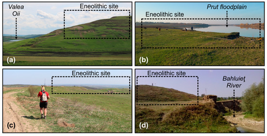
Figure 2.
Images of Eneolithic archaeological sites in the study area: (a) Dealul Mare/Dealul Boghiu settlement (Cucuteni A) on the top of the cuesta landform; (b) field surveys along the Ripiceni–La Holm settlement (Cucuteni A–B) located on the right bank of Prut floodplain; (c) GPS surveys in the plateau-plain transition zone (Siret river basin); (d) Costeşti settlement (Cier/La Şcoală, Cucuteni A) located on a small hill within Bahluieț Valley.
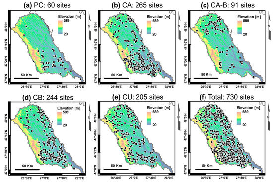
Figure 3.
Eneolithic sites distribution in the study area: (a) Precucuteni; (b) Cucuteni A; (c) Cucuteni A–B; (d) Cucuteni B; (e) Cucuteni settlements with unknown cultural phase; (f) total archaeological sites.
2.2. Elevation Data
The elevation model based on high-density airborne LiDAR (Light Detection and Ranging) data used to analyses the area within the buffer zones (1000 m radius) around each archaeological site was achieved by spatially processing in the ArcGIS software of 730 .tiff files. The rasters were generated in grid formats through Inverse Distance Weighting (IDW) interpolation, with cell sizes of 1 m used for large-scale analysis, and 25 m used for small-scale representations of the study area [64,65,66] (Figure 3). The resulting small-scale DEMs were filtered using flow direction, sink and fill tools, to reduce the errors generated by merging the .tiff files [64,67]. In the large-scale maps, the 25 m DEM resolution was used, where vegetation, buildings, and other artificial structures were filtered before processing the archaeological data. The slope pattern was generated using Spatial Analyst Tools (ArcGIS), and delineation of landform units based on TPI and DEV was performed using Relief Analysis Toolbox for ArcGIS [3,5,55] (Figure 4).
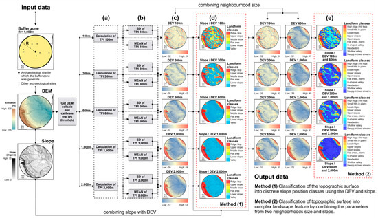
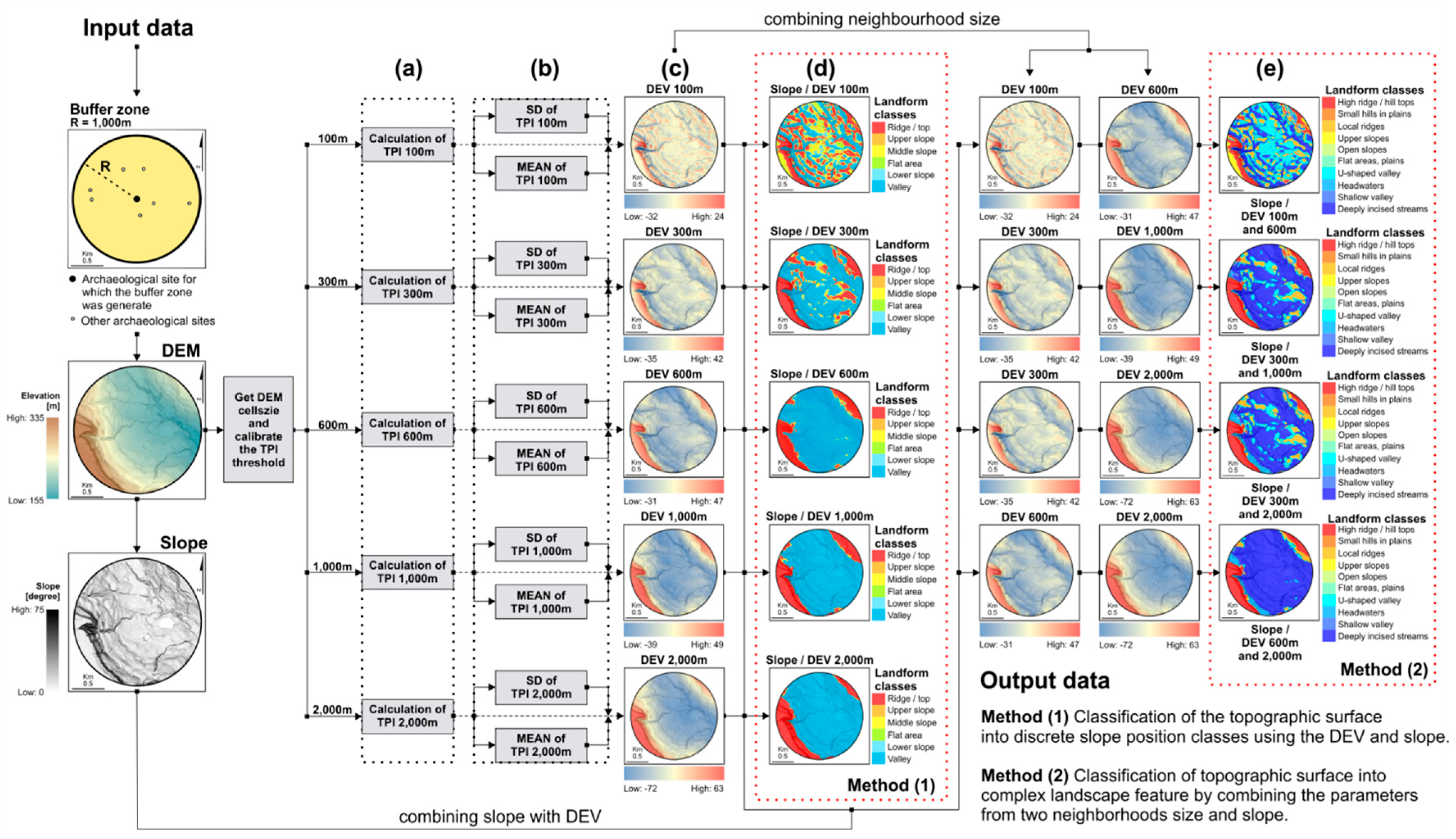
Figure 4.
Workflow chart for the landform classification process—the input data (DEM and Slope) were extracted using a 1000 m buffer zone around an Eneolithic site selected randomly from the study area: (a) calculation of TPI rasters for 100 m, 300 m, 600m, 1000 m, and 2000 m thresholds using the algorithm developed by [3] and [55]; (b) calculation of standardized TPI for each threshold rasters based on SD and Mean after the ArcGIS algorithm described by [75]; (c) generate the DEV models for each threshold rasters based on standardized TPI after [29]; (d) classification of landscape features into six slope position classes using the DEV and slope for each threshold rasters (Method 1) after [3]; (e) classification of landscape features into 10 landform classes by combining the slope with parameters from two neighbourhood sizes (DEV 100 m and 600 m; DEV 300 m and 1000 m; DEV 300 m and 2000 m; DEV 600 m and 2000 m) (Method 2) after [4].
2.3. Flood Hazard Data
To generate the flood hazard pattern in the area of interest, the HEC-RAS v 5.0.1 software (Hydrologic Engineering Centers—River Analysis System), which is an auxiliary module for ArcGIS 10.2, was used [45,68]. The hydrological risk assessment process comprised three steps: (i) the pre-processing step, involving the generation of the thematic layers (thalweg, banks, flow paths, and cross-section vector) based on DEM with a resolution of 0.5m/pixel; (ii) the processing step, involving the export of the thematic layers to the HEC-RAS software and introducing the parameters required to run the flood simulation (Manning roughness coefficient; Flows with an insurances of 0.1%); and (iii) the post-processing step, involving the export of the HEC-RAS result into the ArcGIS software and the generation of the flood extent in order to obtain flood bands with an insurance of 0.1 % (1000 years). The large-scale flood hazard assessment was chosen instead of frequent floods with lower insurance (e.g., 1% or 100 year) because the topographic surface has been anthropogenically modified over time, and this fact disturbs the flood pattern at small-scale.
2.4. Delineation of Landform Units
2.4.1. TPI and DEV
TPI is based on the algorithm developed by Weiss A.D. [3] and implemented as an extension for ESRI ArcView 3.x. by Jenness J. [55]. This tool calculates the difference between elevations at the central point (Equation (1)) and the average elevation (Equation (2)) around it within a known radius R [3,28,29,55,69]. Positive or negative values of TPI indicate that the central point is located higher () or lower (), respectively, than its average surroundings. In this equation, the range of TPI depends not only on distinguishes between and , but also with respect to R, because a large R-value generally reveals large-scale landform units (major valleys, mountains, hills), while smaller values highlight small-scale features (stream valleys, headwaters, local ridges) [4,5,29] (Figure 4a).
In addition to the basic algorithm, DEV measures the using TPI and the standard deviation SD of the elevation (Equation (3)) [29,55]. DEV improves the results because it measures the topographic position as a fraction of local relief normalized to local surface roughness (Equation (4)) [28,29]. As with TPI results, positive values of DEV () indicate that the central point is situated higher than its neighbourhood, and negative values () indicate that it is situated lower [3,69] (Figure 4b).
TPI and DEV are two complementary methods frequently used in archaeological landscape research [70]. However, we consider it most appropriate to use DEV instead of TPI due to the higher potential accuracy of landform classification and the ability to identify the topographic preferences of archaeological settlements in a heterogeneous landscape [29] (Figure 4c).
2.4.2. Landform Classification
There are many algorithms which divide the landscape into geomorphological classes [3,5,71,72,73,74,75]. In this study, the Weiss A.D. [3] method was applied. Method (1): classification of the topographic surface into discrete slope position classes using the DEV [29] (Figure 4d). Method (2): classification of the topographic surface into a complex landscape feature by combining the parameters from two neighbourhood size [4,28] (Figure 4e). The values of five candidate radii for slope position classes (100 m, 300 m, 600 m, 1000 m, and 2000 m), and four different combinations of neighbourhood sizes for classified the landform features (100 m and 600 m; 300 m and 1000 m; 300 m and 2000; 600 m and 2000 m) were used in this paper [3].
3. GIS-Based Landform Classification Results
3.1. Validation of Landform Classification Accuracy for Various Neighbourhood Sizes
The summaries of archaeological site placement classified into six slope position classes using Criterion (1) for five candidate radii are shown in Table 1 and Figure 5. The summaries of archaeological site placement classified into 10 landform classes for the four combined versions of small-TPI and large-TPI neighbourhood sizes according to Criterion (2) are shown in Table 2 and Figure 6.

Table 1.
Number of Eneolithic settlements occurring over six slope position classes in NE Romania; Method (1) (see Figure 4e).
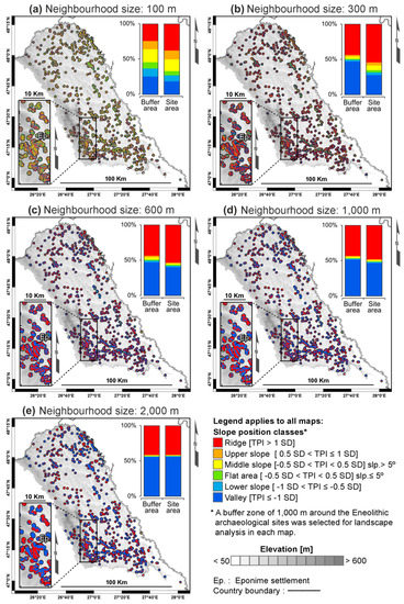
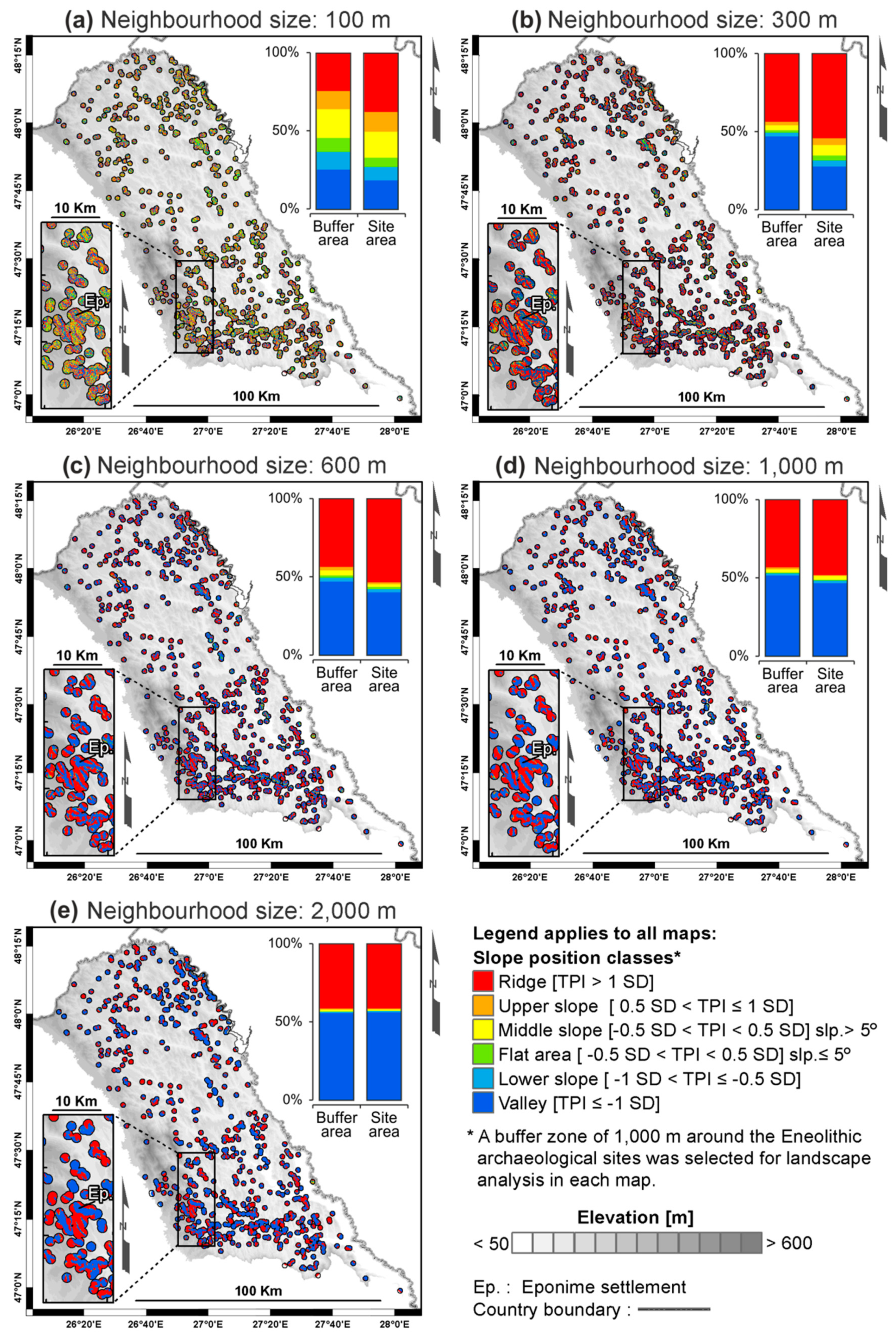
Figure 5.
Slope position classification based on DEV of the case study sites in NE Romania; for the Eneolithic period (chronological framework: ca. 5000–3500 BCE), with six morphological classes for the neighbourhood sizes (a) 100 m, (b) 300 m, (c) 600 m, (d) 1000 m, and (e) 2000 m. The statistics apply to both the buffer zone and site location in each map.
Table 2.
Number of Eneolithic settlements occurring over ten specific landform types in NE Romania; Method (2) (see Figure 4d).
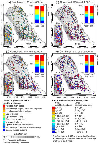
Figure 6.
Landform classification based on DEV of the case study sites in NE Romania, for Eneolithic period (chronological framework: ca. 5000–3500 BCE), with ten landform types for the combined neighbourhood sizes (a) 100 m and 600 m, (b) 300 m and 1000 m, (c) 300 m and 2000 m, (d) 600 m and 2000 m; the statistics apply to both the buffer zone and site location in each map.
The accuracy of the results has been verified using the visual interpretation of aerial imagery and by comparing the landform classification generated by TPI with the specific morphological features of over 100 settlement locations provided by previous geomorphological and archaeological surveys in the study area [39,47,48,49,50,51,52,53,54]. Also, according to [28,29], which applied the same methodology of landscape classification within a heterogenous landscape in Belgium, in this case, the same DEV thresholds and various neighbourhood sizes were used; the results obtained by [28,29] are applicable for our study area, being a plateau-plain transition zone.
For the first method (1), test results indicate that R = 300 m is the most appropriate for the rest of our analyses, because it discriminates the various features with less fragmentation and without a high density of patches (see: R = 100 m), and also without a high degree of generalization (see: R = 600 m, R = 1000 m, and R = 2000 m) (Figure 5). For the second classification method (2), because the topography of the study area is quite rugged, the results of 300 m and 1000 m combined neighbourhood sizes highlight the predominant landform types occupied by Eneolithic settlements. Other results emphasize the flat areas (see: 100 m and 600 m combined neighbourhood sizes), or reduce the classification of landform feature from 10 landform classes in just two main relief features: hilltops and valleys (see: 300 m and 2000 m, and 600 m and 2000 m combined neighbourhood sizes) (Figure 6). The statistical analysis and geoarchaeological interpretation of archaeological site placement per landform classes were achieved based on these two results.
3.2. Classification of Archaeological Site Placement Based on Slope Position
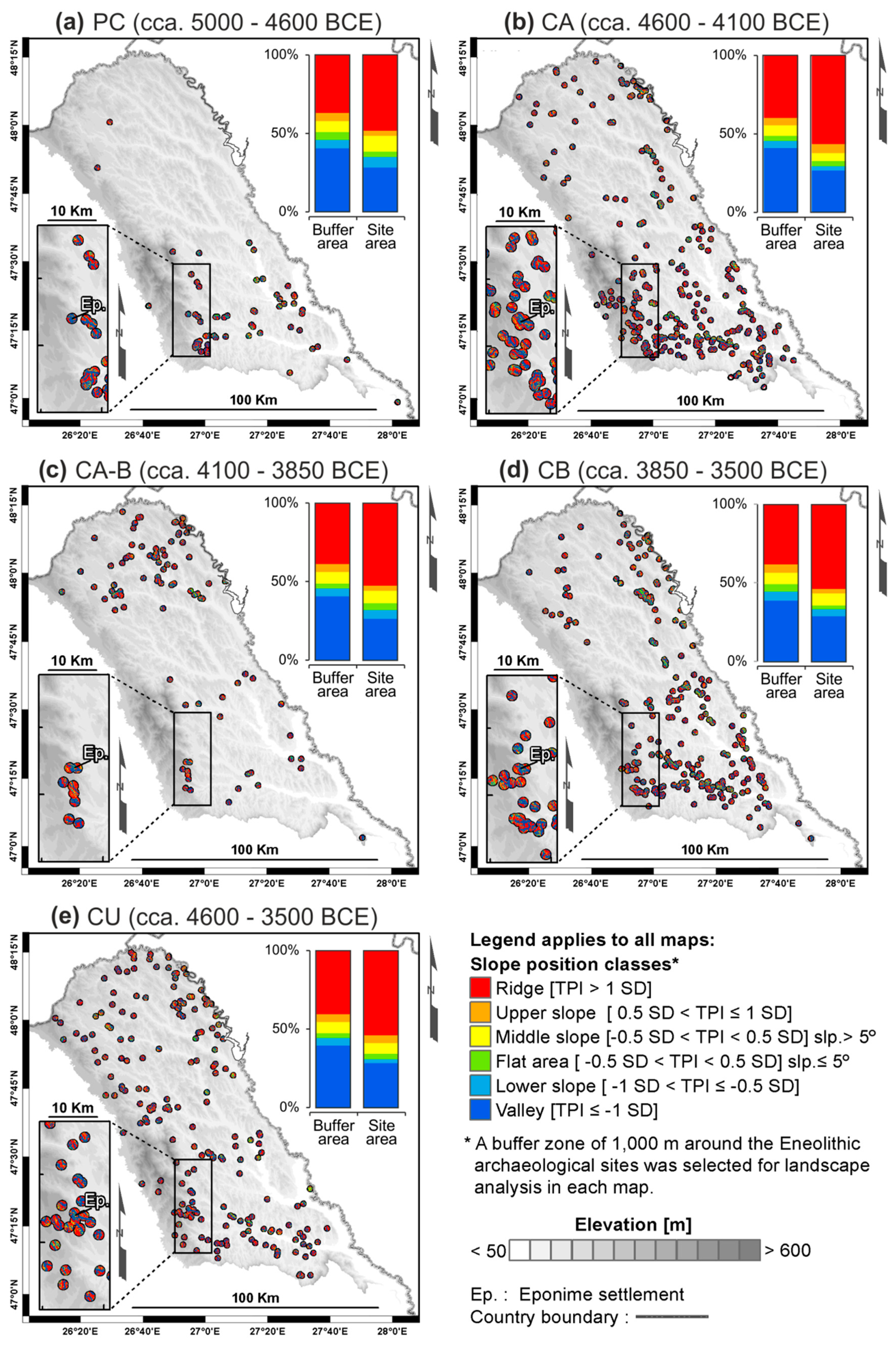
According to the slope position classification generated using SD of TPI (DEV) and R = 300 m, over 65% of settlements were placed on the convex landforms: 470 sites on ridge, summit, or hilltops; 37 sites on upper slopes; 58 sites on middle slopes (>5°); and 28 sites (≤5°) on flat areas. Thirty percent of the settlements were placed on concave features: lower slope, foot slope, 32 sites on toe slopes; and 240 sites in valleys (Figure 7). In the Precucuteni period (ca. 5000–4600 BCE), 48.3% of settlements were located on the top of the hills, 13.3% on upper and middle slopes and the remaining 38.4% of sites preferred flat areas or lower landforms like foot slopes and valleys (Figure 7a). During the Cucuteni period (ca. 4600–3500 BCE), regardless of the cultural phases (Cucuteni A, A–B, or B), the location of settlements seems to follow the same slope position pattern: an average of 54.4% on ridges, summits, and tops 4.2% on upper slopes; 6.7% on middle slopes (>5°); 3.4% on flat areas (≤5°); 3.7% on lower slopes (foot slope, toe slope); and 27.5% in valleys (Figure 7b–e). Overall, the preference of the Eneolithic communities for placing their settlements on the top of cuesta near the steep slope is determined by the necessity to provide defence for at least one or two sides of the settlement. This is the first criterion used by prehistoric communities in the selection of habitation locations based on local topography (Figure 7).
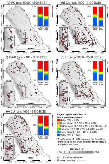
Figure 7.
Slope position classification based on DEV of the case study sites in NE Romania, for (a) PC, (b) CA, (c) CA–B, (d) CB, and (e) CU cultural periods, with six morphological classes for the 300 m neighbourhood sizes; the statistics apply to both the buffer zone and site location in each map.
3.3. Classification of Archaeological Site Placement Based on Landform Units
Based on TPI-landform classification using 300 m and 1000 m combined neighbourhood sizes, 59.5% of sites are located on convex landforms: 348 sites on hilltops, high ridges; 24 sites on middle slope ridges, small hills in the plains; 96 sites on local ridges/hills in the valley; and 47 sites on upper slopes. 1.7% of the sites are located in the flat areas or on the gentle slope surfaces: plains, flat areas (<5°)—7 sites; open slopes (>5°)—7 sites (Figure 8). The remaining of 38.8% of sites overlie concave landforms: 211 sites on deeply incised streams; 6 sites on middle slope drainages, small hills in the plains; 25 sites on upland drainages, headwaters; and 94 sites in U-shaped valleys. The high ridges and hills remained the main landform classes used by prehistoric communities for the location of settlements (average 39%), regardless of the cultural period (Figure 8a–e). The least represented classes are the flat or gentle slope areas (average 0.7%), most likely due to the wetlands, which occupied the flood plain of main rivers and are not suitable for habitation but important for hunting and fishing. Of the concave landform classes, the deeply incised streams (average 24.22%) and U-shaped valleys (average 12.12%) are the most represented, confirming that the second method of defending settlements was to be located in the vicinity of natural channels like stream meanders or steep banks. For the same reason, in 10.9% of cases, the sites are located on the local ridges or small hills in the valley (Figure 8).
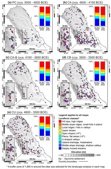
Figure 8.
Landform classification based on DEV of the case study sites in NE Romania, for (a) PC, (b) CA, (c) CA–B, (d) CB, and (e) CU cultural periods, with ten landform types for the 300 m and 1000 m combined neighbourhood sizes; the statistics apply to both the buffer zone and site location in each map.
4. Discussion
4.1. Habitation Practices During the Eneolithic Period
This work has quantified the landform variations of Precucuteni (PC) and Cucuteni (CA, CA–B, CB, and CU) settlement locations in the landscape between Siret and Prut rivers (Moldavian Plain, NE Romania). A general trend is observed throughout the entire Eneolithic period, when the prehistoric communities preferred to place the settlements on the hilltops or in the culmination area.
In this way, the front of cuestas provides a good defence of the settlement, offers a wider perspective on the landscape, and a very good (inter)visibility [47,48,49,50,51,52,53,54]. The sites located in the valleys have a lower relative frequency, and it is possible to correlate their placement with seasonal mobility for the practice of agriculture [35,36,37,75].
The increasing number of sites located on the top of the hills since the end of the Precucuteni period is connected with demographic growth and with a slight climate change which occurred at the beginning of the Cucuteni A period. Compared to the previous Eneolithic phase, the dry period during the Cucuteni caused a decline of subsistence agriculture, forcing human communities to migrate towards the northern part of the Moldavian Plain in search of new fertile lands, pastures and resources (see Cucuteni A–B settlement distribution) [35,75]. Even though in Cucuteni B some of the communities return to the old territories, the slope position pattern remains the same. Due to the heterogeneous landscape which characterizes the area between Siret and Prut rivers, the habitat preferences and the cultural practice, especially those related to subsistence agriculture, did not change significantly during the Eneolithic. From this point of view, the results of this approach highlight the eco-cultural niche occupied by settlement in the Precucuteni and Cucuteni periods in the study area.
Regarding the accuracy of landform classification into discrete slope position classes using the DEV, and by combining the parameters from two neighbourhood sizes using large-TPI and small-TPI, the results indicate a high agreement with the archaeological surveys and landscape description achieved within the study area [34,35,36,37,38]. Even this approach could not replace the classic geomorphological expert opinion, it does bring new insights in remote sensing applied in cultural heritage assessment, preventive archaeology and archaeological predictive modelling.
4.2. Flood Hazard Perception During the Eneolithic Period
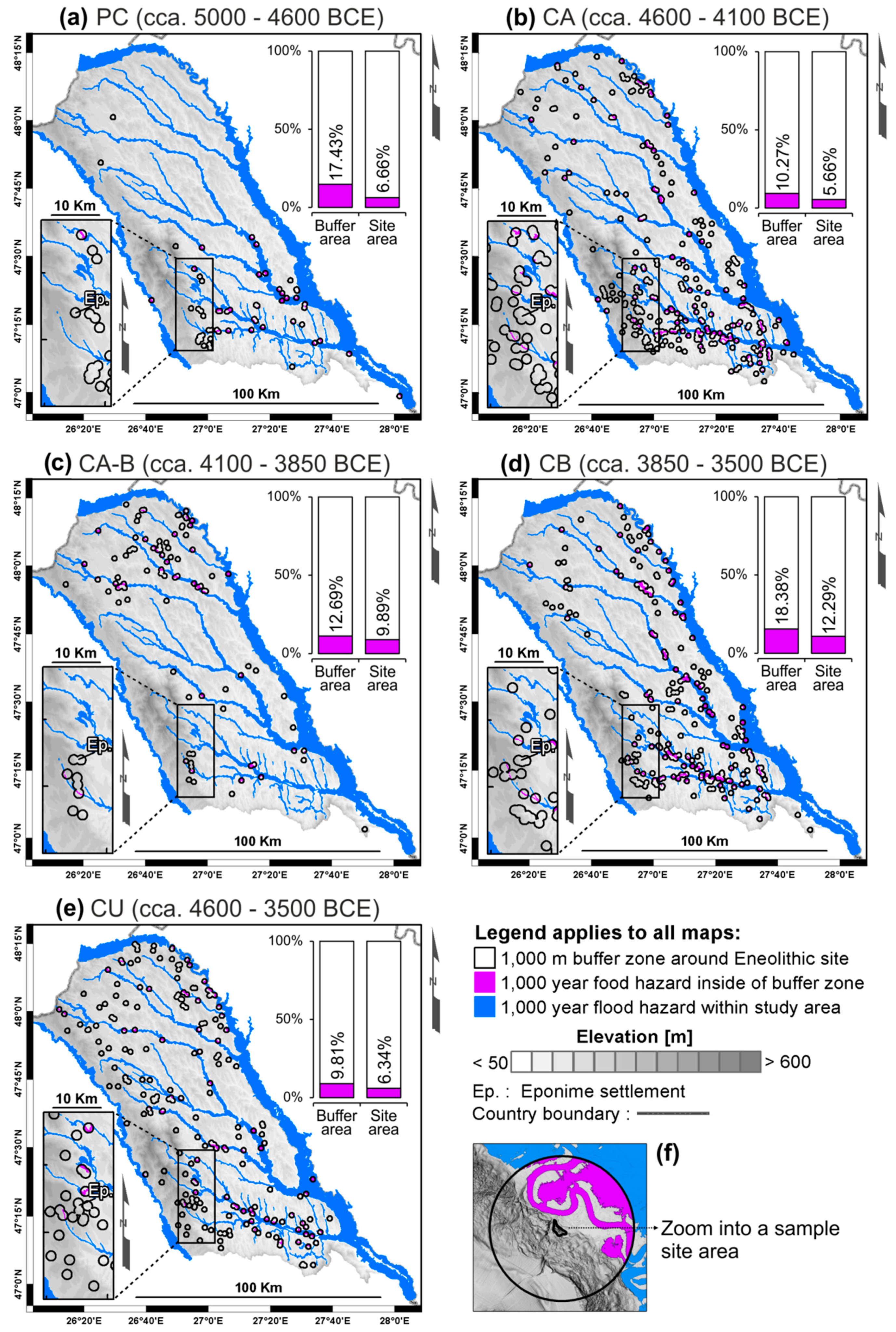
The placement of flooding areas likely indicates that the territories occupied by wetlands were used by prehistoric communities for hunting and fishing, but they are also emphasized as being a very inappropriate habitation place due to floods. According to HEC-RAS flood hazard pattern provided using 1000-year discharge insurance [45,46,49], only 8.2% of the total sites were placed in vulnerable areas (Figure 9). During the Precucuteni and Cucuteni A phases, the settlements potentially affected by high flood events do not exceed 6.5% (Figure 9a,b), in Cucuteni A–B, this value increases to 9.9% (Figure 9c), and during Cucuteni B, the number of vulnerable settlements reaches 12.3% (Figure 9d,e). According to slope position classification generated using SD of TPI (DEV), the most potentially affected settlements are those that were located on the low areas like: valleys (37 sites), lower/middle slopes (12 sites), and flat areas with ≤ 5º slope (13 sites) (Table 3). According to the TPI-landform classification by combining two neighbourhood sizes, the most potentially affected settlements by floods were built on the concave landforms: deeply incised streams (37 sites), U-shaped valleys (25), and plains with ≤ 5° slope (3 sites) (Table 4). These sites may correspond to temporary settlements used for a particular activity (e.g., fishing, hunting, clay exploitation, flint processing), and could indicate the seasonal mobility of prehistoric communities generated by the annual hydrological regimes [34,35,36,37,38,41,75].

Figure 9.
Flood hazard vulnerability generated with 1000 year discharge insurance for the case study sites in NE Romania: (a) PC, (b) CA, (c) CA–B, (d) CB, and (e) CU cultural periods; (f) zoomed-in on a sample site area from Prut floodplain; the statistics apply to both the buffer zone and site location in each map.
Table 3.
Number of Eneolithic settlements occurring over six slope position classes (300 DEV and slope) vs. number of sites which are in the flood hazard area (1000 year flood band insurances) in the NE Romania.
Table 4.
Number of Eneolithic settlements occurring over ten specific landform types (combining 300 DEV and 1000 DEV) vs. number of sites which are in the flood hazard area (1000yr flood band insurances) in the NE Romania.
Overall, the habitation practices deduced from settlement landform patterns attest that prehistoric communities had a high awareness of flood hazard, especially during the Precucuteni and Cucuteni A periods (ca. 5000–4100 BCE). The relative increase of the number of sites placed in the vulnerable areas in the second half of the analysed period (ca. 4100–3500 BCE) can be explained by the migration of inhabited territory to the north and north-east (Cucuteni A–B phase; ca. 4100–3850 BCE) near to the Prut floodplain, the river with the highest hydrological activity in the lowland region. Also, the Cucuteni B phase (ca. 3850–3500 BCE) corresponded with the increase of the prehistoric population, and implicitly, with the territorial expansion of habitation places during the drier periods [48,63]. However, the low-presence of Eneolithic sites in floodplain of the main rivers indicate a relative cyclicality of hydrological events associated with overflow (e.g., seasonal flooding, flash floods), and also highlights the areas affected by excess of humidity (e.g., wetlands or riparian zone), which are unfit for permanent habitation.
5. Conclusions
The geoarchaeological investigation of the heterogeneous landscapes of the Moldavian Plain (NE Romania) using GIS landform classification and flood hazard assessment has produced valuable information regarding the distribution of 730 Precucuteni and Cucuteni settlements during the Eneolithic period. The habitation practices and flood hazard perception results based on DEV (SD of TPI) and HEC-RAS modelling technique applied in this approach are:
- According to slope position classification based on DEV 300 m, over 65% of settlements were placed on the convex landforms (e.g., ridge, summit, hill top), <5% of total settlements on flat areas with a slope ≤ 5°, and 30% of settlements were placed on concave features (e.g., valleys).
- According to the TPI-landform classification by combining two neighbourhood sizes, in this study DEV 300 and DEV 1000, 59.5% of sites are located on positive landforms (e.g., hill tops, high ridges, small hills in plains, local ridges/hills in valley), 1.7 % sites are on the flat areas or on the gentle slope surfaces (< 5°), and 38.8% sites overlap on the negative landforms (e.g., U-shaped valleys, headwaters, shallow valley, deeply incised streams).
- According to flood hazard pattern generated for an extent with 0.1% insurance (1000 years), 8.2% of sites are located in vulnerable areas which indicate a high flood hazard perception during the Eneolithic period.
- The high-density settlements built on specific landforms (e.g., ridge, top of cuestas) indicate a habitation practice during the Eneolithic based on local topography and highlight a specific eco-cultural niche for the prehistoric communities in the plateau-plain transition zone of NE Romania.
Regarding the methodology applied in this approach, the GIS landform classification based on TPI and DEV combined with other morphological variables (e.g., slope) can be integrated very easily into future paleo-environmental, archaeological predictive modelling, and cultural heritage management studies. Furthermore, the difference between conventional archaeological surveys and the GIS techniques used in this work is made by rapid, low-cost and the ability to perform the analysis both at small and large scale.
Author Contributions
Conceptualization, A.M.-P.; methodology, A.M.-P. and I.C.N.; software, I.C.N.; validation, A.M.-P. and I.C.N..; formal analysis, A.M.-P.; investigation, A.M.-P. and I.C.N.; resources, A.M.-P.; data curation, A.M.-P.; writing—original draft preparation, A.M.-P. and I.C.N.; writing—review and editing, A.M.-P. and I.C.N.; supervision, A.M.-P.; project administration, A.M.-P.; funding acquisition, A.M.-P.
Funding
This research and APC was funded by “Alexandru Ioan Cuza” University of Iaşi, within the Research Grants program, grant number GI-UAIC-2018-01: Geoarchaeological approaches in alluvial environments using GIS techniques. An integrated applied research model for Eneolithic settlements from Moldavian Plain (Grant coordinator: A.M.-P.).
Acknowledgments
The authors would like to express their gratitude to the employees of the Romanian Waters Agency Bucharest, Prut-Bîrlad Water Administration Iaşi, particularly to Claudiu Pricop, hydrologist at this research and administration agency, who kindly provided a significant part of the LiDAR data used in the present study. Daniel Joseph Fallu (Tromsø University Museum, UiT the Arctic University of Norway) is kindly acknowledged for the English language editing of the manuscript. All data was processed in the Geoarchaeology Laboratory (Coordinator: A.M.-P.) of Institute for Interdisciplinary Research, Science Research Department, “Alexandru Ioan Cuza” University of Iaşi (UAIC), Romania. Our thanks go to three anonymous reviewers, who helped us in improving the manuscript.
Conflicts of Interest
The authors declare no conflict of interest. The founding sponsors had no role in the design of the study; in the collection, analyses, or interpretation of data; in the writing of the manuscript, and in the decision to publish the results.
Abbreviations
The following abbreviations are used in this manuscript:
| GIS | Geographic Information System |
| GPS | Global Positioning System |
| TPI | Topographic Position Index |
| SD | Standard Deviation |
| DEV | SD of TPI |
| LiDAR | Light Detection and Ranging |
| DEM | Digital Elevation Model |
| IDW | Inverse Distance Weighting |
| HEC-RAS | Hydrologic Engineering Centers—River Analysis System |
| R | Radius |
| Average elevation pixels for various candidate radii | |
| z0 | Central pixel elevation for various candidate radii |
| PC | Precucuteni cultural phase |
| CA | Cucuteni A cultural phase |
| CA–B | Cucuteni A–B cultural phase |
| CB | Cucuteni B cultural phase |
| CU | Cucuteni (unknown cultural phase) |
| BCE | Before Common Era |
References
- Blaszczynski, J.S. Landform characterization with geographic information systems. Photogramm. Eng. Rem. Sens. 1997, 63, 183–191. [Google Scholar]
- Pike, R.J. A Bibliography of Terrain Modeling (Geomorphometry), the Quantitative Representation of Topography—Supplement 4.0. US Geological Survey, 2002; pp. 1–158. Available online: https://pubs.usgs.gov/of/2002/0465/pdf/of02-465.pdf (accessed on 30 March 2019).
- Weiss, A.D. Topographic Position and Landforms Analysis. In Proceedings of the ESRI User Conference, San Diego, CA, USA, 9–13 July 2001; pp. 227–245. Available online: http://www.jennessent.com/downloads/TPI-poster-TNC_18x22.pdf (accessed on 28 January 2019).
- Argyriou, A.V.; Teeuw, R.M.; Sarris, A. GIS-based landform classification of Bronze Age archaeological sites on Crete Island. PLoS ONE 2017, 12, e0170727. [Google Scholar] [CrossRef] [PubMed]
- Deumlich, D.; Schmidt, R.; Sommer, M. A multiscale soil-landform relationship in the glacial-drift area based on digital terrain analysis and soil attributes. J. Plant. Nutr. Soil Sci. 2010, 173, 843–851. [Google Scholar] [CrossRef]
- Illés, G.; Kovács, G.; Heil, B. Comparing and evaluating digital soil mapping methods in a Hungarian forest reserve. Can. J. Soil Sci. 2011, 91, 615–626. [Google Scholar] [CrossRef]
- Mora-Vallejo, A.; Claessens, L.; Stoorvogel, J.; Heuvelink, G.B.M. Small scale digital soil mapping in southeastern Kenya. Catena 2008, 76, 44–53. [Google Scholar] [CrossRef]
- Pracilio, G.; Smettem, K.; Bennett, D.; Harper, R.; Adams, M. Site assessment of a woody crop where a shallow hardpan soil layer constrained plant growth. Plant. Soil. 2006, 288, 113–125. [Google Scholar] [CrossRef]
- Dębniak, K.; Mège, D.; Gurgurewicz, J. Geomorphology of Ius Chasma, Valles Marineris, Mars. J. Maps 2017, 13, 260–269. [Google Scholar] [CrossRef]
- Liu, M.; Hu, Y.; Chang, Y.; He, X.; Zhang, W. Land use and land cover change analysis and prediction in the upper reaches of the Minjiang River, China. Environ. Manag. 2009, 43, 899–907. [Google Scholar] [CrossRef] [PubMed]
- McGarigal, K.; Tagil, S.; Cushman, S. Surface metrics: An alternative to patch metrics for the quantification of landscape structure. Landsc. Ecol. 2009, 24, 433–450. [Google Scholar] [CrossRef]
- Tagil, S.; Jenness, J. GIS-based automated landform classification and topographic, landcover and geologic attributes of landforms around the Yazoren Polje, Turkey. J. Appl. Sci. 2008, 8, 910–921. [Google Scholar] [CrossRef]
- Wilson, M.F.J.; O’Connell, B.; Brown, C.; Guinan, J.C.; Grehan, A.J. Multiscale terrain analysis of multibeam bathymetry data for habitat mapping on the continental slope. Mar. Geod. 2007, 30, 3–35. [Google Scholar] [CrossRef]
- Wright, D.J.; Heyman, W.D. Introduction to the special issue: Marine and coastal GIS for geomorphology, habitat mapping, and marine reserves. Mar. Geod. 2008, 31, 223–230. [Google Scholar] [CrossRef]
- Zieger, S.; Stieglitz, T.; Kininmonth, S. Mapping reef features from multibeam sonar data using multiscale morphometric analysis. Mar. Geol. 2009, 264, 209–217. [Google Scholar] [CrossRef]
- Francés, A.P.; Lubczynski, M.W. Topsoil thickness prediction at the catchment scale by integration of invasive sampling, surface geophysics, remote sensing and statistical modeling. J. Hydrol. 2011, 405, 31–47. [Google Scholar] [CrossRef]
- Lesschen, J.P.; Kok, K.; Verburg, P.H.; Cammeraat, L.H. Identification of vulnerable areas for gully erosion under different scenarios of land abandonment in southeast Spain. Catena 2007, 71, 110–121. [Google Scholar] [CrossRef]
- Liu, H.; Bu, R.; Liu, J.; Leng, W.; Hu, Y.; Yang, L.; Liu, H. Predicting the wetland distributions under climate warming in the Great Xing’an Mountains, northeastern China. Ecol. Res. 2011, 26, 605–613. [Google Scholar] [CrossRef]
- Bunn, A.; Hughes, M.; Salzer, M. Topographically modified tree-ring chronologies as a potential means to improve paleoclimate inference. Clim. Chang. 2011, 105, 627–634. [Google Scholar] [CrossRef]
- Fei, S.; Schibig, J.; Vance, M. Spatial habitat modeling of American chestnut at Mammoth Cave National Park. For. Ecol. Manag. 2007, 252, 201–207. [Google Scholar] [CrossRef]
- Guitet, S.; Cornu, J.-F.; Brunaux, O.; Betbeder, J.; Carozza, J.-M.; Richard-Hansen, C. Landform and landscape mapping, French Guiana (South America). J. Maps 2013, 9, 325–335. [Google Scholar] [CrossRef]
- Berking, J.; Beckers, B.; Schütt, B. Runoff in two semi-arid watersheds in a geoarcheological context: A case study of Naga, Sudan, and Resafa, Syria. Geoarchaeology 2010, 25, 815–836. [Google Scholar] [CrossRef]
- Nicu, I.C. Application of analytic hierarchy process, frequency ratio, and statistical index to landslide susceptibility: An approach to endangered cultural heritage. Environ. Earth Sci. 2018, 77, 79. [Google Scholar] [CrossRef]
- Patterson, J.J. Late Holocene land use in the Nutzotin Mountains: Lithic scatters, viewsheds, and resource distribution. Arctic Anthropol. 2008, 45, 114–127. [Google Scholar] [CrossRef]
- Noviello, M.; Cafarelli, B.; Calculli, C.; Sarris, A.; Mairota, P. Investigating the distribution of archaeological sites: Multiparametric vs probability models and potentials for remote sensing data. Appl. Geogr. 2018, 95, 34–44. [Google Scholar] [CrossRef]
- Brouwer Burg, M. Reconstructing “total” paleo-landscapes for archaeological investigation: An example from the central Netherlands. J. Archaeol. Sci. 2013, 40, 2308–2320. [Google Scholar] [CrossRef]
- Llobera, M. Building past landscape perception with GIS: Understanding topographic prominence. J. Archaeol. Sci. 2001, 28, 1005–1014. [Google Scholar] [CrossRef]
- De Reu, J.; Bourgeois, J.; De Smedt, P.; Zwertvaegher, A.; Antrop, M.; Bats, M.; De Maeyer, P.; Finke, P.; Van Meirvenne, M.; Verniers, J.; et al. Measuring the relative topographic position of archaeological sites in the landscape, a case study on the Bronze Age barrows in northwest Belgium. J. Archaeol. Sci. 2011, 38, 3435–3446. [Google Scholar] [CrossRef]
- De Reu, J.; Bourgeois, J.; Bats, M.; Zwertvaegher, A.; Gelorini, V.; De Smedt, P.; Chu, W.; Antrop, M.; De Maeyer, P.; Finke, P.; et al. Application of the topographic position index to heterogeneous landscapes. Geomorphology 2013, 186, 39–49. [Google Scholar] [CrossRef]
- Kvamme, K.L. One-Sample Tests in Regional Archaeological Analysis: New Possibilities through Computer Technology. Am. Antiq. 1990, 55, 367–381. [Google Scholar] [CrossRef]
- Kvamme, K.L. Terrain form analysis of archaeological location through geographic information systems. In Computer Applications and Quantitative Methods in Archaeology 1991, BAR International Series; Lock, G., Moffett, J., Eds.; Tempus Reparatum: Oxford, UK, 1992; pp. 127–136. [Google Scholar]
- Hung, C.-L.J.; James, L.A.; Hodgson, M.E. An automated algorithm for mapping building impervious areas from airborne LiDAR point-cloud data for flood hydrology. Gisci. Remote Sens. 2018, 55, 793–816. [Google Scholar] [CrossRef]
- Toda, L.L.; Yokingco, J.C.E.; Paringit, E.C.; Lasco, R.D. A LiDAR-based flood modelling approach for mapping rice cultivation areas in Apalit, Pampanga. Appl. Geogr. 2017, 80, 34–47. [Google Scholar] [CrossRef]
- Lazarovici, C.M.; Lazarovici, G.; Turcanu, S. Cucuteni: A Great Civilization of the Prehistoric World; Editura Palatul Culturii: Iaşi, Romania, 2009; pp. 1–350. [Google Scholar]
- Mantu, C.M. Cultura Cucuteni. Evoluţie, Cronologie, Relaţii Culturale; Editura Nona: Piatra Neamt, Romania, 1998; pp. 1–324. [Google Scholar]
- Mantu, C.M. Cucuteni-Tripolye cultural complex: Relations and synchronisms with other contemporaneous cultures from the Black Sea area. Stud. Antiq. Archaeol. 2000, 7, 11–27. [Google Scholar]
- Monah, D.; Monah, F. The last great Chalcolithic civilization of Old Europe. In Cucuteni. The Last Great Chalcolithic Civilization of Old Europe; Mantu, C.M., Dumitroaia, G.H., Tsaravopoulos, A., Eds.; Athena Publishing & Printing House: Bucharest, Romania, 1997; pp. 15–98. [Google Scholar]
- Ursulescu, N. Cucuteni-Tripillya: The space of a civilization. In Cucutenie-Tripillya: A Great Civilization of Old Europe; Exhibition Catalog of Mineniul III Foundation and Hers Consulting Group: Vatican, Italy, 2008; pp. 15–20. [Google Scholar]
- Asăndulesei, A. Inside a Cucuteni Settlement: Remote Sensing Techniques for Documenting an Unexplored Eneolithic Site from Northeastern Romania. Remote Sens. 2017, 9, 41. [Google Scholar] [CrossRef]
- Măţău, F.; Nica, V.; Postolache, P.; Ursachi, I.; Cotiuga, V.; Stancu, A. Physical study of the Cucuteni pottery technology. J. Archaeol. Sci. 2013, 40, 914–925. [Google Scholar] [CrossRef]
- Tencariu, F.-A.; Alexianu, M.; Cotiuga, V.; Vasilache, V.; Sandu, I. Briquetage and salt cakes: An experimental approach of a prehistoric technique. J. Archaeol. Sci. 2015, 59, 118–131. [Google Scholar] [CrossRef]
- Băcăuanu, V. Câmpia Moldovei. Studiu Geomorfologic; Editura Academiei Romane: Bucuresti, Romania, 1968; pp. 1–222. [Google Scholar]
- Mărgărint, M.C.; Niculiţă, M. Landslide Type and Pattern in Moldavian Plateau, NE Romania. In Landform Dynamics and Evolution in Romania; Radoane, M., Vespremeanu-Stroe, A., Eds.; Springer Geography, Springer: Cham, The Netherlands, 2017; pp. 271–304. [Google Scholar] [CrossRef]
- Niculiţă, M. A landform classification schema for structural landforms of the Moldavian platform (Romania). In Geomorphometry; Hengl, T., Evans, I.S., Wilson, J.P., Gould, M., Eds.; Geomorphometry.org: Redlands, CA, USA, 2011; pp. 129–132. [Google Scholar]
- Romanescu, G.; Cîmpianu, C.I.; Mihu-Pintilie, A.; Stoleriu, C.C. Historic flood events in NE Romania (post-1990). J. Maps 2017, 13, 787–798. [Google Scholar] [CrossRef]
- Romanescu, G.; Mihu-Pintilie, A.; Stoleriu, C.C.; Carboni, D.; Paveluc, L.; Cîmpianu, C.I. A Comparative Analysis of Exceptional Flood Events in the Context of Heavy Rains in the Summer of 2010: Siret Basin (NE Romania) Case Study. Water 2018, 10, 216. [Google Scholar] [CrossRef]
- Brigan, R.; Weller, O. Neo-Eneolithic settlement pattern and salt exploitation in Romanian Moldavia. J. Archaeol. Sci. Rep. 2018, 17, 68–78. [Google Scholar] [CrossRef]
- Niculiţă, M.; Mărgărint, M.C.; Santangelo, M. Archaeological evidence for Holocene landslide activity in the eastern Carpathian lowland. Quat. Int. 2016, 415, 175–189. [Google Scholar] [CrossRef]
- Mihu-Pintilie, A.; Asăndulesei, A.; Stoleriu, C.C.; Romanescu, G. GIS methods for assessment of hydro-geomorphic risk and anthropogenic impact which affect the archaeological sites. Case study: Dealul Mare archaeological site, Moldavian Plateau (Romania). Acta Geobalcanica 2016, 2, 35–43. [Google Scholar] [CrossRef]
- Nicu, I.C. Cultural heritage assessment and vulnerability using Analytic Hierarchy Process and Geographic Information Systems (Valea Oii catchment, North-eastern Romania). An approach to historical maps. Int. J. Disaster Risk. Reduct. 2016, 20, 103–111. [Google Scholar] [CrossRef]
- Nicu, I.C.; Romanescu, G. Effect of natural risk factors upon the evolution of Chalcolithic human settlements in Northeastern Romania (Valea Oii watershed). From ancient times dynamics to present days degradation. Z. Geomorphol. 2016, 60, 1–9. [Google Scholar] [CrossRef]
- Nicu, I.C. Frequency ratio and GIS-based evaluation of landslide susceptibility applied to cultural heritage assessment. J. Cult. Herit. 2017, 28, 172–176. [Google Scholar] [CrossRef]
- Nicu, I.C. Is overgrazing really influencing soil erosion? Water 2018, 10, 1077. [Google Scholar] [CrossRef]
- Nicu, I.C. Natural risk assessment and mitigation of cultural heritage sites in North-eastern Romania (Valea Oii river basin). Area 2019, 51, 142–154. [Google Scholar] [CrossRef]
- Jenness, J. Topographic Position Index (tpi_jen.avx) extension for ArcView 3.x, v. 1.2. Jenness Enterprises. Available online: http://www.jennessent.com/arcview/tpi.htm (accessed on 31 March 2019).
- Drăguţ, L.; Blaschke, T. Automated classification of landform elements using object-based image analysis. Geomorphology 2006, 81, 330–344. [Google Scholar] [CrossRef]
- MacMillan, R.A.; Pettapiece, W.W.; Nolan, S.C.; Goddard, T.W. A generic procedure for automatically segmenting landforms into landform elements using DEMs, heuristic rules and fuzzy logic. Fuzzy Sets Syst. 2000, 113, 81–109. [Google Scholar] [CrossRef]
- Bates, M.R.; Wenban-Smith, F.F. Palaeolithic Geoarchaeology: Palaeolandscape Modelling and Scales of Investigation. Landscapes 2011, 12, 69–96. [Google Scholar] [CrossRef]
- Verhagen, P.; Whitley, T.G. Integrating Archaeological Theory and Predictive Modeling: A Live Report from the Scene. J. Archaeol. Method Theory 2012, 19, 49–100. [Google Scholar] [CrossRef]
- Warren, R.E.; Asch, D.L. A Predictive model of archaeological site location in the Eastern Prairie Peninsula. In Practical Applications of GIS for Archaeologists. A Predictive Modeling Toolkit; Wescott, K.L., Brandon, R.J., Eds.; Taylor & Francis: London, UK, 2000; pp. 3–32. [Google Scholar]
- Windler, A.; Thiele, R.; Müller, J. Increasing inequality in Chalcolithic Southeast Europe: The case of Durankulak. J. Archaeol. Sci. 2012, 40, 204–210. [Google Scholar] [CrossRef]
- Haase, D.; Fink, J.; Haase, G.; Ruske, R.; Pécsi, M.; Richter, H.; Altermann, M.; Jäger, K.-D. Loess in Europe—Its spatial distribution based on a European loess map, scale 1:250,000. Quat. Sci. Rev. 2007, 26, 1301–1312. [Google Scholar] [CrossRef]
- Rădoane, M.; Constantin, N.; Chiriloaei, F.; Rădoane, N.; Popa, I.; Roibu, C.-C.; Roibu, D. Late Holocene fluvial activity and correlations with dendrochronology of subfossil trunks: Case studies of northeastern Romania. Geomorphology 2016, 239, 142–159. [Google Scholar] [CrossRef]
- Doneus, M. Openness as visualization technique for interpretative mapping of airborne LiDAR derived digital terrain models. Remote Sens. 2013, 5, 6427–6442. [Google Scholar] [CrossRef]
- Lu, G.Y.; Wong, D.W. An adaptive inverse-distance weighting spatial interpolation technique. Comput. Geosci. 2008, 34, 1044–1055. [Google Scholar] [CrossRef]
- Zimmerman, D.; Pavlik, C.; Ruggles, A.; Armstrong, M.P. An experimental comparison of ordinary and universal Kriging and Inverse Distance Weighting. Math. Geol. 1999, 31, 375–390. [Google Scholar] [CrossRef]
- Zhou, T.; Popescu, S.; Malambo, L.; Zhao, K.; Krause, K. From LiDAR Waveforms to Hyper Point Clouds: A Novel Data Product to Characterize Vegetation Structure. Remote Sens. 2018, 10, 1949. [Google Scholar] [CrossRef]
- Patel, C.G.; Gundaliya, P.J. Floodplain delineation using HEC-RAS model—A case study of Surat City. Open J. Modern Hydrol. 2016, 6, 34–42. [Google Scholar] [CrossRef]
- Gallant, J.C.; Wilson, J.P. Primary Topographic Attributes. In Terrain Analysis: Principles and Applications; Wilson, J.P., Gallant, J.C., Eds.; Wiley: New York, NY, USA, 2000; pp. 51–85. [Google Scholar]
- Crombé, P.; Sergant, J.; Robinson, E.; De Reu, J. Hunter-gatherer responses to environmental change during the Pleistocene–Holocene transition in the southern North Sea basin: Final Palaeolithic–Final Mesolithic land use in northwest Belgium. J. Anthropol. Archaeol. 2011, 30, 454–471. [Google Scholar] [CrossRef]
- Burrough, P.A.; van Gaans, P.F.M.; MacMillan, R.A. High-resolution landform classification using fuzzy k-means. Fuzzy Sets Syst. 2000, 113, 37–52. [Google Scholar] [CrossRef]
- Deng, Y. New trends in digital terrain analysis: Landform definition, representation, and classification. Prog. Phys. Geogr. 2007, 31, 405–419. [Google Scholar] [CrossRef]
- Iwahashi, J.; Pike, R.J. Automated classifications of topography from DEM’s by an unsupervised nested-means algorithm and a three-part geometric signature. Geomorphology 2007, 86, 409–440. [Google Scholar] [CrossRef]
- Nikitin, A.G.; Ivanova, S.; Kiosak, D.; Badgerow, J.; Pashnick, J. Subdivisions of haplogroups U and C encompass mitochondrial DNA lineages of Eneolithic-Early Bronze Age Kurgan populations of western North Pontic steppe. J. Hum. Genet. 2017, 62, 605–613. [Google Scholar] [CrossRef] [PubMed]
- Becker, D.; de Andrés-Herrero, M.; Willmes, C.; Bareth, G.; Weniger, G. GIS-Based Automated Landform Classification for Analysis of Archaeological Sites. Collaborative Research Centre 806, 2014. Available online: https://crc806db.uni-koeln.de (accessed on 28 January 2019).


© 2019 by the authors. Licensee MDPI, Basel, Switzerland. This article is an open access article distributed under the terms and conditions of the Creative Commons Attribution (CC BY) license (http://creativecommons.org/licenses/by/4.0/).