The Near-Space Wind and Temperature Sensing Interferometer: Forward Model and Measurement Simulation

Abstract

Wind and temperature observation in near space has been playing an increasingly important role in atmospheric physics and space science. This paper reports on the near-space wind and temperature sensing interferometer (NWTSI), which employs a wide-angle Michelson interferometer to observe O₂(a¹Δ_g) dayglow near 1.27 μm from a limb-viewing satellite, and presents the instrument modeling and observation simulations from the stratosphere to the mesosphere and lower thermosphere. The characteristics of atmospheric limb-radiance spectra and line selection rules are described. The observational strategy of using two sets of three emission lines with a line-strength difference of one order of magnitude is proved to be suitable for extending altitude coverage. The forward modeling and measurement simulation of the expected NWTSI observations are provided, and the measurement uncertainty of the wind and temperature is discussed. The signal-to-noise ratio (SNR) and the limb-view weight work together to affect the precision of the wind and temperature measurements. The simulated results indicate a wind measurement precision of 1 to 3 m/s and a temperature precision of 1 to 3 K over an altitude range from 40 to 80 km, which meets the observing requirement in measurement precision for near-space detection.

1. Introduction

Near space is generally defined as an altitude range from 20 km to the “edge of space”—the Kármán line—at 100 km, and has started to play an increasingly important role in atmospheric physics and space science [1]. Wind and temperature are two extremely important physical quantities to characterize the atmosphere parameters of the near space. Both wind and temperature measurements are of great scientific significance for studying the semiannual oscillation of the middle atmosphere [2], global structure, and seasonal variability of the migrating diurnal tide [3], the momentum and energy fluxes of monochromatic gravity waves [4], and the planetary waves excited by wind interaction with topography [5]. In addition, sensitive observations of atmospheric wind and temperature have great practical value for improving the accuracy of environmental prediction, ensuring aerospace safety, and achieving a higher satellite launch success rate.

For a long time, the detection of atmospheric wind and temperature has been largely restricted to ground-based remote sensing technologies, such as Doppler wind light detection and ranging (LIDAR) [6], Raman temperature LIDAR [7], meteor radar [8], and airglow imaging interferometer [9]. The continuous development of space technology creates favorable conditions for observing wind and temperature from satellites. The spaceborne airglow imaging interferometer measures the atmospheric wind and temperature globally by detecting the broadening, frequency shift, and intensity change of the airglow spectrum from limb-viewing satellites, and therefore provides greatly enhanced vertical spatial resolution. Due to traction needs, spaceborne wind and temperature interferometry is becoming the frontier topic of the satellite remote sensing field [10].

Wind calculation is obtained from the Doppler frequency shift of the airglow by measuring the phase change of the interferogram, and the temperature is usually calculated from the Doppler broadening by analyzing the interferogram contrast change. The phase change of the interferogram is more sensitive than the contrast change, leading to a higher accuracy for wind inversion (about 5 to 8 m/s) than for temperature measurement (about 20 to 75 K). For airglow emissions from diatomic or polyatomic molecules, the atmospheric temperature can also be determined from the relative intensities of two isolated emission lines if the emission is in the thermodynamic equilibrium with the ambient atmosphere. The two-line ratio method has been proven to yield greater accuracy for temperature measurements (about 1 to 3 K). The Wind Imaging Interferometer (WINDII) [11] on the Upper Atmosphere Research Satellite (UARS) measured wind and temperature in the altitude range from 75 to 320 km using the red line (630.0 nm) and green line (557.7 nm) of the O atom and rotational lines in the atmospheric A band (762 nm) of the O₂ molecule. On the same satellite, the High-Resolution Doppler Imager (HRDI) is loaded to detect the atmospheric wind and temperature from the stratosphere (10 to 40 km) to the mesosphere and lower thermosphere (50 to 120 km) with the absorption and emission characteristics of three vibrational bands, (0,0), (1,0), and (2,0) in the $b^1{\mathsf{\Sigma }}_g^{+}\leftarrow X^3{\mathsf{\Sigma }}_g^{-}$ transition of the O₂ molecule, achieving a wind measurement accuracy of about 5 m/s [12] and a temperature accuracy of about 7 K [13].

The remarkable success of WINDII and HRDI stimulates interest in taking atmospheric wind and temperature at lower altitudes to yield more altitude coverage. A concept for an instrument called the Stratospheric Wind Interferometer for Transport studies (SWIFT) was developed by employing the Doppler Asymmetric Spatial Heterodyne (DASH) approach and using the vibration–rotation ozone line at 1133.4335 cm^-1 as the Doppler target for the stratospheric wind measurement. [14,15]. The Doppler Wind and Temperature Sounder (DWTS) instrument employs gas filter correlation radiometry technology, and was initiated to simultaneously measure the Doppler shift and the linewidth of emission spectra to infer both wind and kinetic temperatures day and night continuously from 25 km to over 250 km [16]. The design strategy of using middle-wave infrared (MWIR) and long-wave infrared (LWIR) emission lines enables the all-time observation capability of SWIFT and DWTS for measuring near-space wind and temperature. However, spaceborne infrared remote sensor systems working in MWIR or LWIR wavebands usually have high instrument thermal backgrounds arising from the lenses, mirrors, and other optical elements in the optical train, and therefore require a low refrigerating temperature, which may lead to an increase of risk, measurement uncertainty, and platform requirements. In addition, SWIFT shows a low ability for temperature measurement, and simulations indicate that DWTS wind measurements only include the cross-tracking component between 50–100 km, and the uncertainty of along-track wind is typically 10 times greater than that of cross-track wind from 100 to 250 km.

A science impact study conducted relying on the Canadian Middle Atmosphere Model [17] resulted in a recommendation that desired accuracies with upper limits in error levels of 5 to 10 m/s for wind and 5 to 10 K for temperature with horizontal resolution better than 400 to 600 km could improve the data assimilation analyses as used in weather forecasting systems [18,19,20,21]. Using the (0,0) vibrational transition of the O₂ infrared atmospheric band (${\mathrm{a}}^1{\Delta }_g\to X^3{\mathsf{\Sigma }}_g$) near 1.27 μm as the Doppler target meets this observing requirement for near-space detection. The O₂(a¹Δ_g) dayglow is suitable for detecting wind and temperature at an altitude range from 45 to 90 km due to its relatively strong radiation and weak self-absorption [22]. The Mesospheric Imaging Michelson (MIMI) deployed by Canada’s StaSci program and the Waves Michelson Interferometer (WAMI) supported by NASA’s MIDEX program are expected to measure wind and temperature using the strong and weak groups of emission lines (three lines in each group) in the O₂ infrared atmospheric band [23].

In this paper, we propose the near-space wind and temperature sensing interferometer (NWTSI) for simultaneous measurements of the atmospheric temperature and wind in the near space by employing a wide-angle Michelson interferometer to observe O₂(a¹Δ_g) dayglow near 1.27 μm from a limb-viewing satellite. Following the WAMI and MIMI concepts, NWTSI pays attention to lower altitudes, from the stratosphere to the mesosphere and lower thermosphere. Since it combines the Doppler Michelson interferometer with the two-line ratio method for rotational temperature measurement, both the accuracies of wind and temperature can therefore be expected to be at high levels. Section 2 explains the characteristics of atmospheric limb-radiance spectra and line selection rules. The instrument concept is described in Section 3. The simulation of the expected NWTSI observations are described in Section 4. The measurement uncertainty of the wind and temperature is discussed in Section 5. A concluding summary in Section 6 completes this paper.

2. Measurement Mechanism

2.1. Characteristics of Atmospheric Limb-Radiance Spectra

The 1.27-μm dayglow provides one of the best spectral features for the remote sensing of global atmospheric temperature and wind due to its bright signal and extended altitude coverage [24]. Emissions of molecular oxygen from the first excited state O₂(a¹∆_g) to the ground state O₂(X³Σ_g) dominate the 1.27-μm dayglow. Accompanied by the occurrence of the electronic transition, energy-level transitions between vibration and rotation states take place simultaneously, which makes the 1.27-μm O₂ dayglow a spectrum band containing about 150 emission lines.

The limb-radiance spectra of the O₂(a¹∆_g) dayglow is calculated by a path integral along the line-of-sight path. The atmosphere is divided into many discrete thin layers, each of which is considered to be uniform. For a line-by-line code, the radiative transfer equation evaluated on the layer-by-layer basis can be expressed as [22]:

$$L{(\nu )}_l=L{(\nu )}_{l-1}\exp (-{\displaystyle \sum \alpha {(\nu )}_{l,i}{u}_l})+\frac{{\displaystyle \sum _{i}J{(\nu )}_{l,i}\alpha {(\nu )}_{l,i}{u}_l}}{{\displaystyle \sum _i\alpha {(\nu )}_{l,i}{u}_l}}[1-\exp (-{\displaystyle \sum _i\alpha {(\nu )}_{l,i}{u}_l})]$$

(1)

where J(ν)_l,i and α(ν)_l,i are the radiation source function and absorption coefficient of path segment i in the layer l, u_l=n_l(Z_U-Z_L) is the molecular column density of O₂ of layer l, n_l is the molecular number density of O₂ in layer l, and Z_U and Z_L are the limb tangent heights of the upper and lower boundaries of the atmosphere l layer, respectively.

Figure 1 shows the limb radiation and transmittance spectra of the O₂ infrared atmospheric band for tangent heights of 40 km, 60 km, and 80 km ignoring the atmospheric wind and the satellite velocity. The three graphs with red lines on the left represent the limb radiation spectrum (Figure 1a,c,e), and the three graphs with blue lines on the right relate to the transmittance spectra (Figure 1b,d,f). As can be seen, emission lines in the center of the band have stronger radiation intensity, while the self-absorption effect is much weaker for rotational lines in the red and blue far wing, and both the emission intensity and the absorption degree vary with tangent heights. This makes the emission lines in the wing candidates for wind and temperature detection at a low-altitude range, and emission lines in the middle suitable for high altitude.

2.2. Line Selection

The first step in the development of the spaceborne wind-temperature imaging interferometer is to select the optimal emission lines, and William E. Ward et al. developed the systematic line-selection criteria [23]. For this work, we use the HITRAN 2012 database [25] and limb radiation transmission characteristics for imaging interferometer design. The spatial and spectral distributions of the two groups of emission lines determined by the line-selection criteria are shown in Figure 2. Figure 2a,b describes three lines of the strong group in the range of 7908 to 7912 cm⁻¹, and Figure 2c,d shows three lines of the weak line group in the range of 7820 to 7824 cm⁻¹. Figure 2a,c and Figure 2b,d show the variation of line intensity and spectral integral intensity in relation to height in the range of 20 to 120 km, respectively.

The emission lines selected for the NWTSI instrument follow three principles: high temperature sensitivity, good spectral separation, and large altitude coverage. Firstly, it is necessary to select a group of spectral lines that are located in different vibration bands with sufficiently different lower-state energy to ensure high temperature sensitivity. In Figure 2a,c, the color of the three-dimensional image represents the intensity of the glow. As illustrated on the whole, three emission lines in each group are found to peak at middle altitude from 40 km to 70 km with slow declines above and below their peaks, which is caused by the low density of the O₂(a¹∆_g) number at high and low altitudes. However, the trend of each emission line with altitude differs hugely in detail, which is due to the difference in the low-state energies. As expected, a large difference in low-state energy is capable for providing high temperature sensitivity. Secondly, good line separation is desired to reduce the requirement in spectral resolution, which would greatly increase the engineering feasibility of temperature and wind measuring interferometers. As can be seen from Figure 2a,c, the three emission lines in both the strong and weak groups are relatively well separated from each other, which allows them to be optically isolated. Finally, extended altitude coverage is expected. To achieve this goal, the observing strategy of using two sets of emission lines with different intensity variations and absorption characteristics as functions of altitude is put forward. The strong line group has strong radiation in the altitude range from 20 km to 90 km (Figure 2a), but suffers from a strong self-absorption effect below 60 km (Figure 2b). Meanwhile, the weak emission lines are suitable for wind and temperature measurement at low altitude due to their relative weak self-absorption effect. So, the NWTSI instrument uses strong lines to sample the atmosphere from 60 to 120 km and the weak lines to sample from 20 to 65 km. The combination of strong and weak emission lines allows the NWTSI instrument access to cover the near space.

3. Instrument Characterization

The NWTSI is a limb-viewing satellite instrument with alternate observations from two orthogonal view directions at azimuths of 45° and 135° from the satellite velocity vector. The pointing mirror points the field of view (FOV) to the corresponding direction between the two measurements, which enables the NWTSI to view approximately the same volume of atmosphere about nine minutes later for a nominal satellite at an altitude of 650 km. 1.5° FOV covers an altitude range from 20 to 120 km, which is just the spatial extension of the near space.

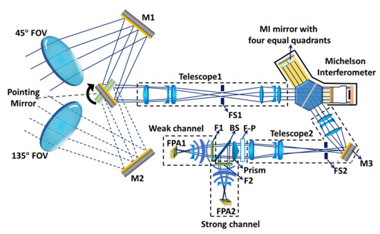
Figure 3 shows the schematic diagram of the optical system for the NWTSI instrument, which closely follows the WAMI concept [23]. The NWTSI consists of two telescopes, a Michelson interferometer, the combination of a narrow-band filter and a Fabry–Perot etalon, and a near-infrared camera. The FOV is defined by telescope 1 and the field stop (FS1). The incoming light is directed by the pointing mirror to telescope 1 and then passed to the Michelson interferometer. The angular magnification of the first telescope is two, which makes the FOV 3° × 3° at the Michelson interferometer. In order to avoid errors caused by intensity variations during measurements, the four interferogram samples are taken simultaneously rather than sequentially. For this policy, the Michelson mirror of the long path arm (LPA) is divided into four equal parts, three of which are coated with different thickness of SiO₂ thin films. The change in the optical path difference (OPD) from one partition to the next is λ/4, which ensures that the optimum step sizes are λ/4, λ/2, and 3λ/4 in OPD for the four segments of the Michelson mirror. For the purposes of step size calibration and permitting the realignment of the interferometer’s mirrors during flight, the mirror of the short path arm (SPA) is mounted on piezoelectrics controlled through a capacitive position sensor. The plane mirror M3 is used to fold the optical element into a compact shape. The angular magnification of telescope 2 is 0.5, so the FOV at the filter system is again 1.5° × 1.5°. The role of the composite of etalon and interference filter is to isolate the target O₂ emission lines from the forest of stratospheric spectral lines and block the scattered sunlight background at the same time. The second telescope focuses on the pyramid prism just behind the filter. The edges of the prism are aligned with the four divisions of the Michelson mirror and projected onto different regions of the focal plane array (FPA), each region of which corresponds to different step phases.

The system parameters for the NWTSI instrument involved in the simulation are provided in

Table 1. System parameters for the NWTSI instrument. OPD: optical path difference, LPA: long path arm, SPA: short path arm.

Component	Parameter	Value and Unit
Satellite	Nominal altitude	650 km
	Distance to limb	2864 km
	Velocity	7533 m/s
Michelson interferometer	OPD	7.35 cm
	Length of LPA	12.24 cm
	Length of the SPA	11.07 cm
	Index of refraction of LPA	1.6605 (LaKN12)
	Index of refraction of SPA	1.504 (BK7)
Fabry–Perot etalon	Free spectral range	2.0 nm
	Finesse	20
	Index of refraction	1.447 (fused silica)
Detector	Format	256 × 256
	Pixel size	40 μm
	Quantum efficiency	0.75
	Dark current	55 electrons/s/pixel
	Readout noise	30 electrons
Instrument responsivity	Pixel étendue	5.25 × 10-10 m2/sr
	Single exposure time	1 s
	Integration time	10 s

.

4. Forward Simulation

This section presents the NWTSI simulated images as would be observed at the detector and discusses the performance assessment of the instrument. The forward model, which was developed to produce the expected interference images, is the theoretical expression for simulating the functions and effects of the instrument. It consists of the atmospheric radiance module, the Michelson phase and filter transmittance function, the attenuation and responsivity of the optical system, and the parameters of the imaging optics, sensor arrays, and camera electronics. Through measurement simulations, we can independently analyze the instrumental properties and study the performance assessment.

4.1. Forward Model

The pixel-level values of the interferogram images are determined as $L(\nu )$, which is the output of the atmospheric model from Equation (1). The equation representing the interferogram for a given pixel is [26]:

$$I_{klj}=R_{lj}{\displaystyle {\int }_{{\nu }_1}^{{\nu }_2}{f}_{lj}(\nu )\cdot L_{lj}(\nu )\cdot \left[1+U_{lj}\cos (2\pi \nu {\Delta }_{lj}+{\phi }_{klj})\right]d\nu }$$

(2)

where I is interferogram of the pixel, $f_{lj}(\nu )$ is the relative total filter function, $U_{lj}$ is the instrument visibility, ${\Delta }_{lj}$ is the OPD, ${\phi }_{klj}$ is the Michelson interferometer kth phase step, ν is the wavenumber, and the instrument responsivity $R_{lj}$ is defined by [27]:

$$R_{lj}=\frac{A\mathsf{\Omega }t\tau q}{hc{\nu }_0}$$

(3)

where AΩ is the étendue of the optical system, t is the integration time, q is the quantum efficiency of the detector, h is Planck’s constant, c is the speed of light in a vacuum, τ is the transmittance of the filter and optical system, and ${\nu }_0$ is the center wavenumber of the O₂ emission line.

For accurate wind measurements, a large field of view (to obtain a large responsivity) is required. Increasing the size of the input solid angle Ω yields a gain in responsivity, but leads to increased OPD variation, which reduces the contrast of the fringes and degrades the desired spectrum. So, there is a limit on the solid angle of the acceptance for the conventional instrument. For the NWTSI instrument (as shown in Figure 3), the FOV at the limb is 1.5° × 1.5°. The angular magnification of the first telescope is two, which makes the FOV 3° × 3° at the Michelson interferometer. The principle of field widening makes it possible for the Michelson interferometer to overcome this limitation, and results in a large étendue even at a large resolving power (high resolution). However, the solid angle of the Fabry–Perot etalon is limited by ${\mathsf{\Omega }}_{\mathrm{FP}}=2\pi n^2/R_{FP}$, where $R_{FP}={\sigma }_0/\delta {\sigma }_{FP}$ is the resolving power of the Fabry–Perot etalon. For this reason, the angular magnification of telescope 2 is designed to be 0.5, so the FOV is again 1.5° × 1.5° for the Fabry–Perot Interferometer.

Imaging the interferogram onto an array detector at four phase steps is the method called four-point sampling of pixel-by-pixel measurement. The interferogram for each pixel is sampled by the camera at four points corresponding to the four phase steps, from which the phase shift in the interferogram due to Doppler wind is obtained. For the NWTSI instrument, the four images are produced by consecutively applying the four phase steps following Equation (2), and the four phase steps are taken simultaneously by using the shallow, pyramid-shaped prism.

4.1.1. Filter Transmittance Function

The O₂(a¹Δ_g) dayglow spectrum near 1.27 μm contains many closely spaced lines. To isolate the target emission lines from this dense spectrum, the effective bandwidth of the filter system has to be about 0.1 nm. A Fabry–Perot filter used in tandem with a narrow band interference filter is necessary to produce a narrow enough passband to isolate each line set. In addition, the narrow-band filter also plays an active role in reducing the level of background light in order to maintain good fringe contrast.

For the NWTSI instrument, each component of its filter system consists of a narrow-band filter and a Fabry–Perot etalon. The total filter function comes from the filter functions of the individual filter components. The optical transmission spectrum of the Fabry–Perot etalon [27] can be modeled by an Airy function and the filter parameters given in Table 1.

$$t(\sigma ,\theta )=\frac{{(1-r)}^2}{1+r^2-2r\cos [\sigma (4\pi {\mathrm{n}}_{etal}\mathrm{d}\mathrm{c}\mathrm{o}\mathrm{s}\theta )]}$$

(4)

where σ is the wavenumber of the incoming light, r is the reflectivity of the filter, n_etal is the refractive index of the etalon material, d is the thickness of the material, and θ is the angle of the refraction inside the Fabry–Perot cavity.

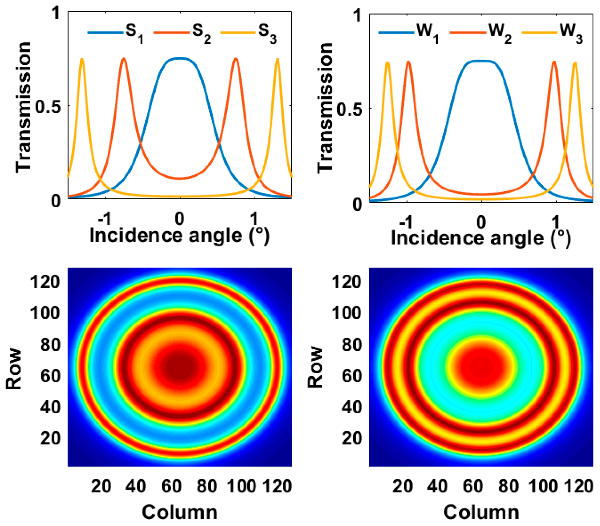
In order to obtain temperature information from the relative intensity ratios of the emitting species, the NWTSI is designed to view three O₂ spectral lines simultaneously over the same FOV. For the reason of reducing the overall cost, a single Fabry–Perot allowing the separation of both the O₂ weak and O₂ strong lines is required. Figure 4 provides the optimum transmittance function of the three weak and strong lines. The optical parameters of the Fabry–Perot etalon are given in Table 1.

4.1.2. Michelson Interferometer Phase

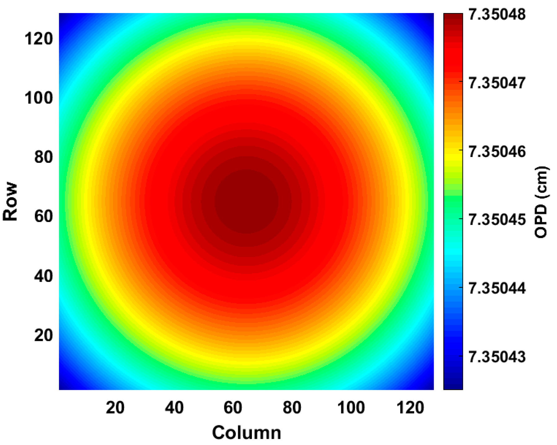
The OPD of the Michelson interferometer varying with the off-axis angle is given by [26]:

$$\Delta (i)\cong 2(n_L{t}_L-n_S{t}_S)-(\frac{{\mathrm{t}}_S}{n_S}-\frac{t_L}{n_L}){\sin }^{2}i-(\frac{{\mathrm{t}}_S}{n_S^3}-\frac{t_L}{n_L^3})\frac{{\sin }^{4}i}{4}-(\frac{{\mathrm{t}}_S}{n_S^5}-\frac{t_L}{n_L^5})\frac{{\sin }^{6}i}{8}$$

(5)

where $n_L$ and $n_S$ are the refractive indexes of the longer and shorter arms, i is the off-axis angle for each pixel (relative to the axis of the Michelson), and t_L and t_S are the length of the longer and shorter arms, respectively. The optical parameters of the Michelson interferometer are given in Table 1. Applying these equations for each pixel, the OPD of each pixel is obtained, which is shown in Figure 5.

The nominal phase steps (k-1)/2π, where k = 1 to 4, refer to the stepping of the geometric central position of each FOV. The mirror phase of the kth phase step for each pixel is expressed as [27]:

$${\phi }_k(i)=(k-1)\times 4\pi \times [\frac{\pi /2}{4\pi d{\nu }_0}]d\times {\nu }_0\cos i$$

(6)

where d is the incremental step of the Michelson phase stepper.

Applying these equations corresponding to the Michelson phase and filter transmittance function for each pixel, and taking the limb spectral radiance shown in Figure 2 into account, the interferogram images will be obtained.

4.2. Measurement Simulation

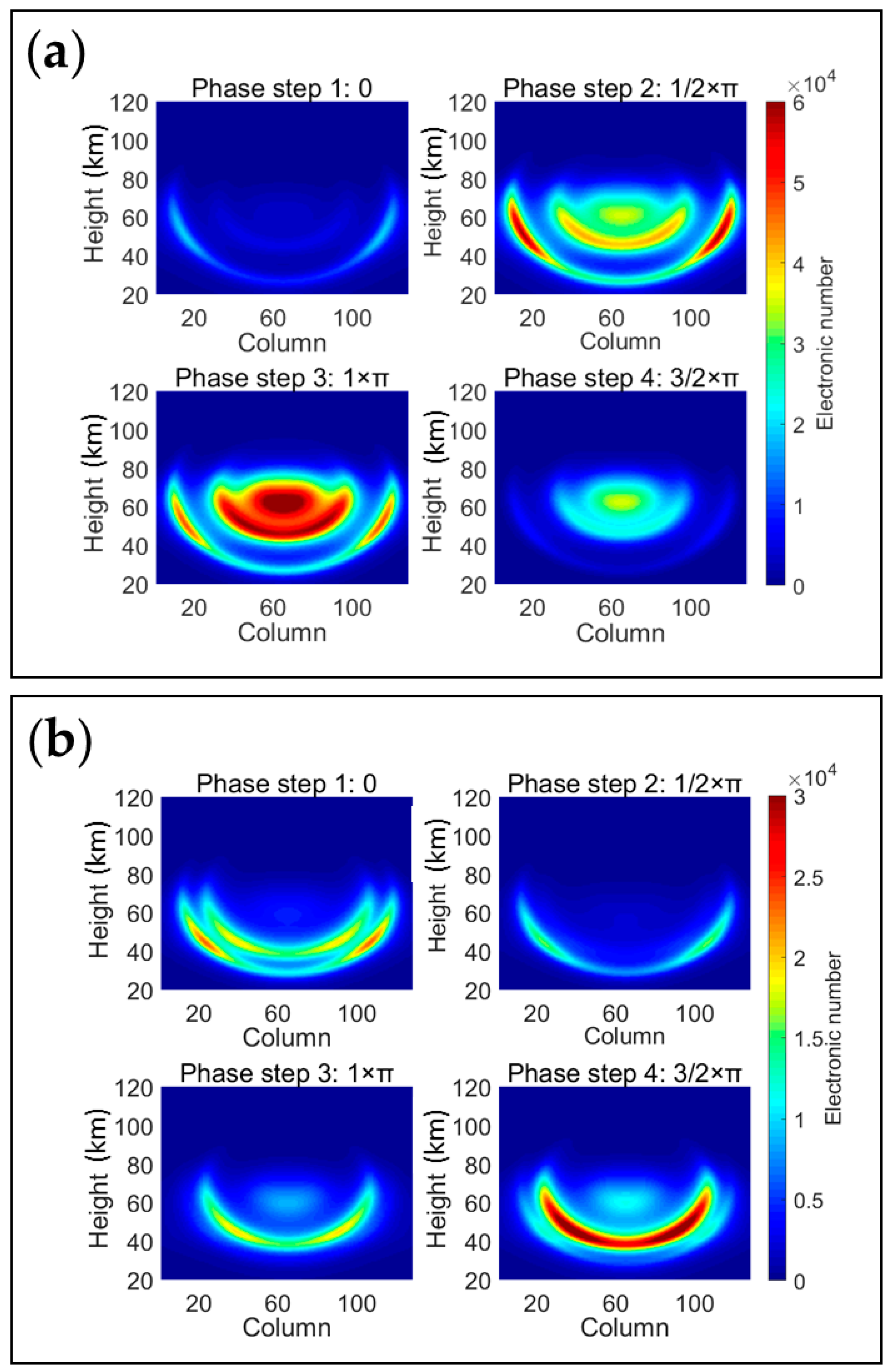
The simulated interferogram images of the weak and strong groups for the four phase steps are shown in Figure 6. The patterns on the interferogram images reflect the dependence of the optical path difference on the pixel positions and phase steps, the variation of the filter transmittance function over the FOV, and the atmospheric spectral radiances varying with tangent height. Each pixel in the interferogram image represents the integral intensity of the limb radiance corresponding to the projected spatial element, which for the NWTSI instrument is about 1 km × 1 km. The differences in the patterns of the images emerge because of the airglow intensity varying with the tangent height and the modulation of the interferogram. For this simulation, the airglow spectral radiance only accounts for variations in the vertical direction; the FOV tilt relative to the horizon and the curvature of the earth are also ignored, and the instrument visibility and responsivity are assumed to be the same for all the pixels.

For each pixel at row l and column j of the detector, its total phase of the interferogram can be found from the four-point sampling method. By removing the earth rotation phase, satellite phase, and instrument phase from the total phase, its phase resulting from wind can be obtained independently. Compared with ground-based observations, the pixel étendue for the limb-viewing instrument is much smaller. However, the long integration path through the limb yields radiances that are much larger than those viewed from the ground.

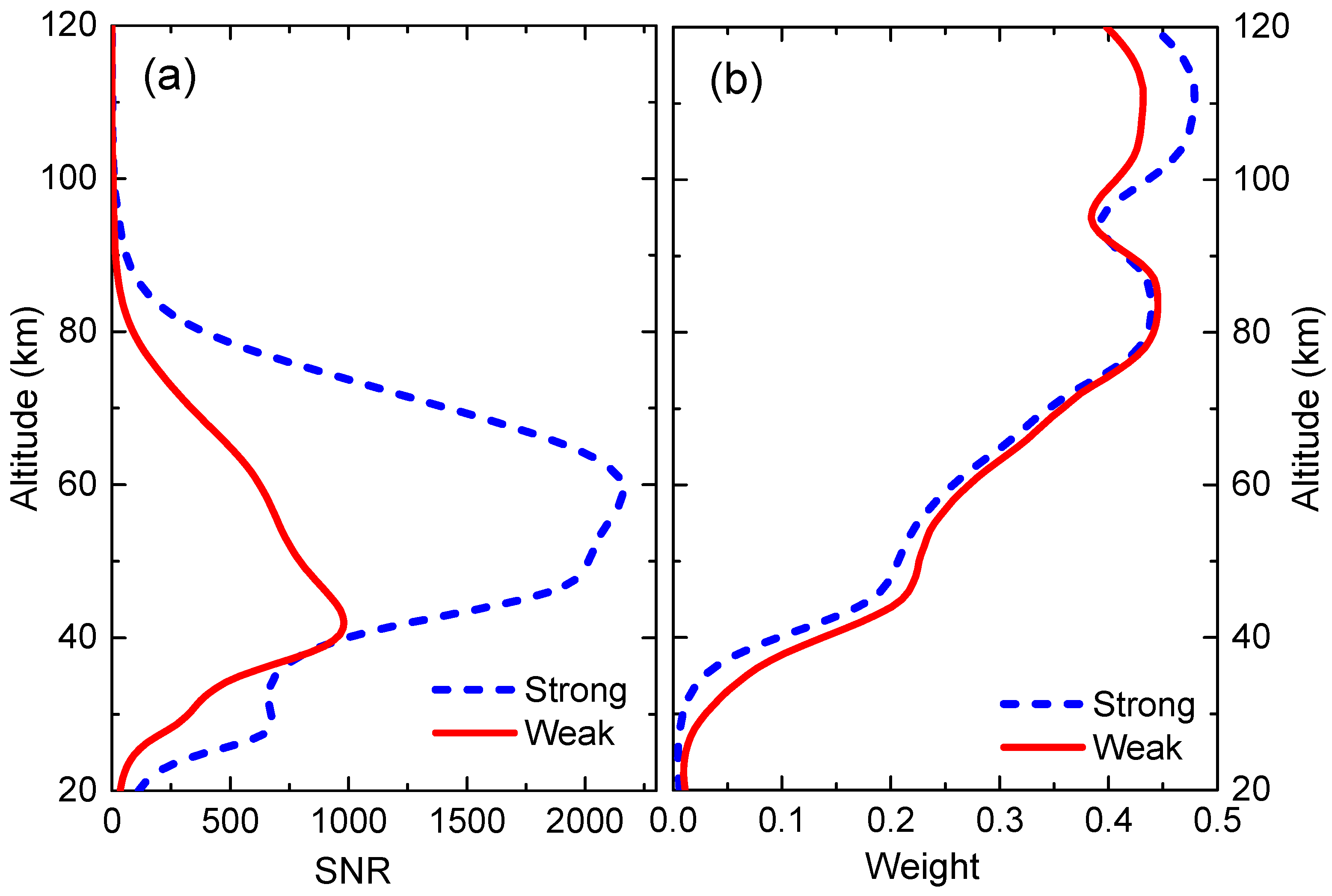
The signal-to-noise ratio (SNR) and the limb-view weight work together to affect the precision of the wind and temperature measurements. Here, limb-view weight means the proportion of the tangent spectral integral intensity in the limb radiance, and SNR refers to the amplitude of the interference fringes from the Michelson. Three major noise sources including shot noise, readout noise, and detector dark noise are taken into account in the simulation of the interferogram images, with specifications listed in Table 1. 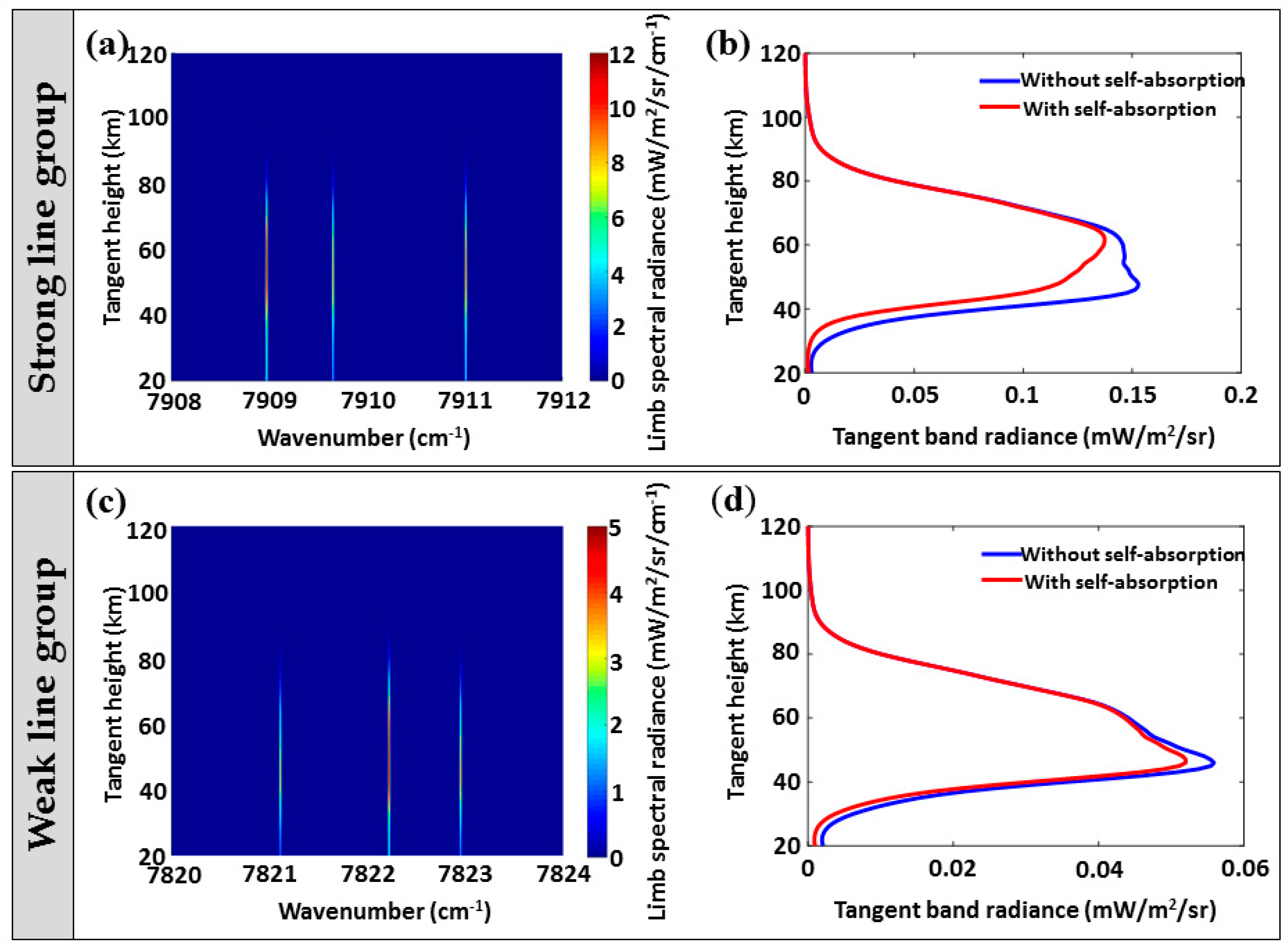The SNR and weight profiles of the weak and strong groups varying with the tangent altitude are illustrated in Figure 7. As can be seen, there is an SNR peak with a value of about 1000 at around 40 to 45 km for the weak group, a slow decline above this peak, and a much more rapid decline below the peak. The SNR of the strong group is found to peak at a higher altitude (about 60 km). The limb-view weight decreases with the tangent height reduction, resulting from the attenuation of the O₂(a¹Δ_g) state density due to collisional quenching at low tangent height.

5. Random Error Estimates

The measurement uncertainty of the wind and temperature values can be determined from a propagation of errors analysis. Both wind and temperature are derived from the Fourier coefficients J₁, J₂, and J₃, which are also referred to as the apparent quantities. The line-of-sight wind is calculated from J₂ and J₃, and the atmospheric temperature is determined by J₁. Using the assumption that all the independent variables are uncorrelated, we can determine the uncertainty in the measured wind and temperature.

The pixel interferogram can be expressed as a truncated Fourier series in terms of the incremental change in optical path difference. Fourier coefficients, J₁, J₂, and J₃, which are also referred to as the apparent quantities, are related to any point k along a fringe interferogram I [28].

$$\begin{array}{l}{J}_1=I_{mean}=\frac{1}{4}{\displaystyle \sum _{k=1}^4{I}_k}\\ J_2=\frac{1}{2U}{\displaystyle \sum _{k=1}^4{I}_k}\cos ({\phi }_{klj})\\ J_3=\frac{1}{2U}{\displaystyle \sum _{k=1}^4{I}_k}\sin ({\phi }_{klj})\end{array}$$

(7)

5.1. Wind Error

The wind velocity $v_w$ is measured as a phase shift $\delta \phi$ of the interferogram [26].

$$v_w=\frac{c}{2\pi \Delta {\nu }_0}\delta \phi$$

(8)

where c is the speed of light, and the phase $\phi$ can be calculated from [27]:

$${\phi }_t={\tan }^{-1}(\frac{J_3}{J_2})$$

(9)

The line-of-sight wind can be obtained for each pixel, and the corresponding standard deviation can be calculated. The random variance of the Doppler wind ${\sigma }_{\nu }^2$ is found from the relation [26]:

$${\sigma }_{\nu }^2=c^2{(2\pi {\nu }_0\Delta )}^{-2}(J_2^2{\sigma }_{J_3}^2+J_3^2{\sigma }_{J_2}^2){(J_2^2+J_3^2)}^{-2}$$

(10)

where J₂ and J₃ are the Fourier coefficients, and ${\sigma }_{J_2}^2$ and ${\sigma }_{J_3}^2$ represent the random variance of the Fourier coefficients.

Figure 8 shows the random error profiles of the line-of-sight wind for the NWTSI instrument by using the emission lines in the strong and weak groups. As can be seen, the line-of-sight wind derived from weak emission lines is more precise than the strong group for lower altitudes (below 42 km), but the reverse is true at higher altitudes. The strong self-absorption of the strong emission lines accounts for this phenomenon, as shown in Figure 1.

5.2. Temperature Error

The atmospheric temperature is determined from the ratio of the integrated absorbances of two isolated emission lines with different temperature dependence [29]:

$$T=\frac{\frac{hc}{k_B}\left({E^{″}}_2-{E^{″}}_1\right)}{\ln \frac{A_1}{A_2}+\ln \frac{S_2\left(T_0\right)}{S_1\left(T_0\right)}+\frac{hc}{k_B}\frac{\left({E^{″}}_2-{E^{″}}_1\right)}{T_0}}$$

(11)

where ${E^{″}}_{}$ (cm⁻¹) is the lower-state energy of the transition, $S_0\left(T\right)$ (cm⁻²·atm⁻¹) is the line strength at the reference temperature T₀=296 K, A is the integral absorbance of the emission line, and h and k_B are Plank’s constant and Boltzmann’s constant, respectively.

The uncertainty of the temperature is determined by the uncertainty of the line strengths and the measured integral absorbances, and can be written as [30]:

$${\sigma }_T=\frac{\Delta T}{T}=\frac{R_A}{T}\frac{dT}{d{R}_A}\sqrt{{\sigma }_{s_1}^2+{\sigma }_{s_2}^2+{\sigma }_{A_1}^2+{\sigma }_{A_2}^2}$$

(12)

where ${\sigma }_{s_{}}^2$ and ${\sigma }_A^2$ represent the random variances of the line strength and the integrated absorbance, and R_A is the ratio of the measured integral absorbances of the two isolated emission lines, R_A=A₁/A₂.

The uncertainty of the measured integrated absorbance is mainly from the signal-to-noise ratio of the mean value of the interferogram, J₁. The line-strength uncertainty results from the error propagation of inherent uncertainty $\Delta S(T_0)$ and temperature-dependent uncertainty $\Delta S_T(T)$. $\Delta S(T_0)$ can be obtained from the HITRAN database [25], while $\Delta S_T(T)$ is proportional to the line strength, which is given by [30]:

$$\Delta S_T^2(T)=S_{}^2(T_0)\Delta T^2\left[-\frac{dQ(T)}{dT}\frac{1}{Q(T)}-\frac{1}{T}+\frac{hc{E}^{″}}{k_B{T}^2}+\frac{hc{\nu }_0}{k_B{T}^2}\left(\frac{\exp (-hc{\nu }_0/k_{B}T)}{1-\exp (-hc{\nu }_0/k_{B}T)}\right)\right]$$

(13)

where Q(T) is the molecular partition function.

Figure 9 shows the temperature error profiles of the NWTSI instrument by using three emission lines in the strong and weak groups. This indicates a random error level in the range of 1.5 to 2 K and 2 to 3 K at the tangent height from 40 to 75 km for the weak and the strong groups. The large values at higher tangent heights are because of the very weak signal at these tangent heights.

6. Conclusions

The NWTSI instrument achieves the simultaneous measurement of wind and temperature by observing O₂(a¹Δ_g) dayglow near 1.27 μm from a limb-viewing satellite, as has been proposed in this paper. The instrument and targeted observations closely follow the WAMI concept published by Ward et al. [23]. Unlike other wind and temperature interferometers such as WINDII and HRDI, we focus our efforts on improving the accuracies of wind and temperature in the near space to a higher level, especially for lower altitude, by using two sets of three emission lines with a line-strength difference of one order of magnitude and combining the Doppler Michelson interferometer with the rotational temperature measurement. 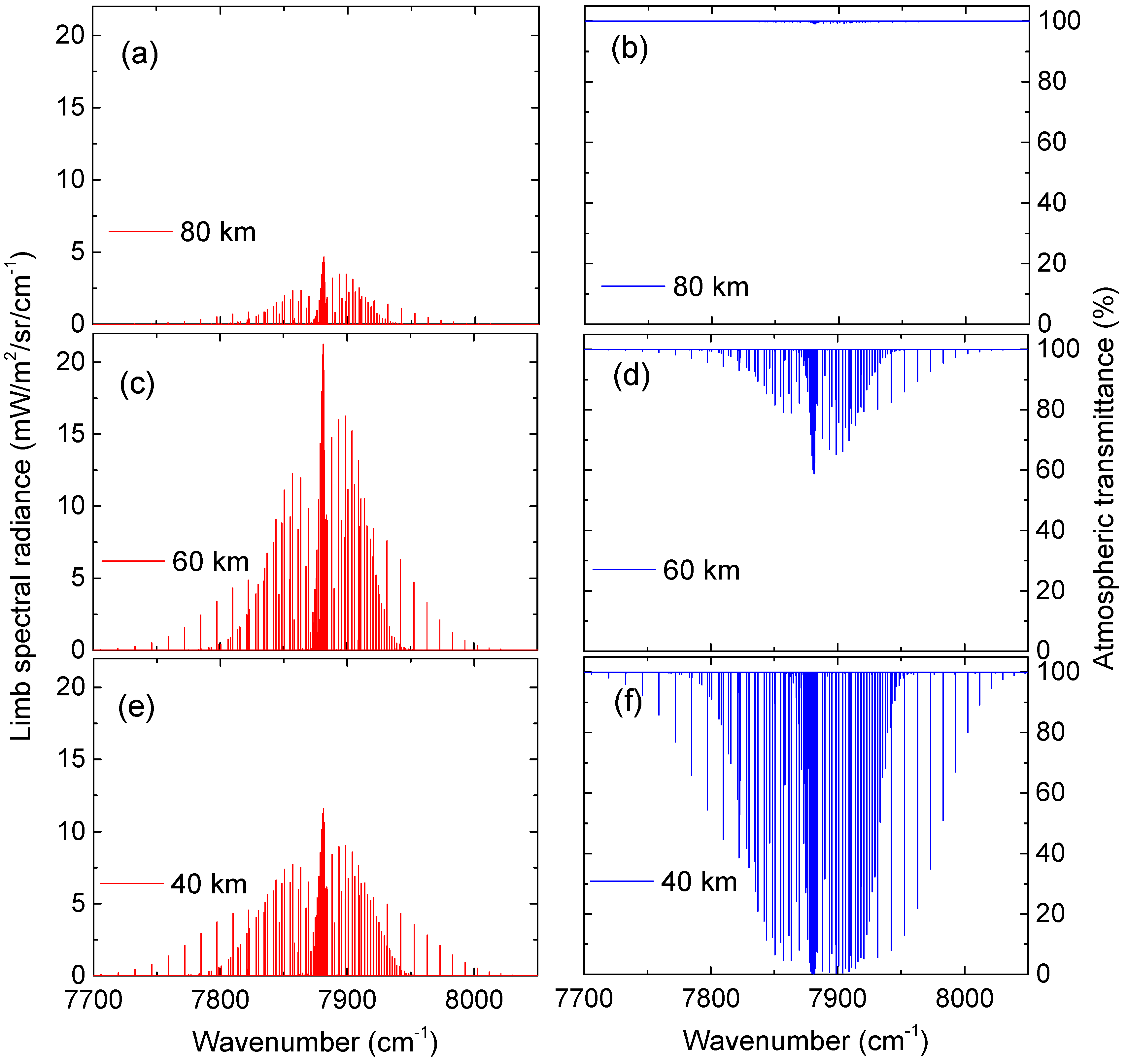The radiative transfer model to calculate the limb-radiance spectra of the O₂(a¹Δ_g) dayglow in the case of limb viewing is developed by using the line-by-line algorithm and the photochemical model incorporating the most recent spectroscopic parameters, rate constants, and solar fluxes. The weak group over the range of 7820 to 7824 cm⁻¹ and the strong group within 7908 to 7912 cm⁻¹ are chosen as an optimum combination for sensitive temperature and wind measurements due to their high-temperature sensitivity, spectral separation, and large altitude coverage. The forward model consisting of the atmospheric radiance module, Michelson phase and filter transmittance function, attenuation and responsivity of the optical system, and optical parameters of the imaging optics, sensor arrays, and camera electronics is developed to produce the expected interference images for simulating the functions and effects of the instrument. The signal-to-noise ratio and the limb-view weight work together to affect the precision of the wind and temperature measurements. 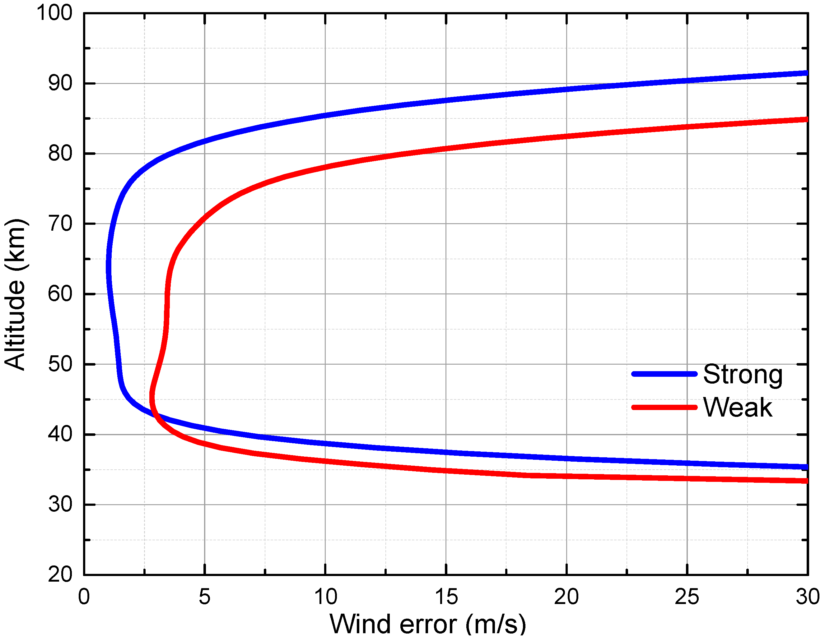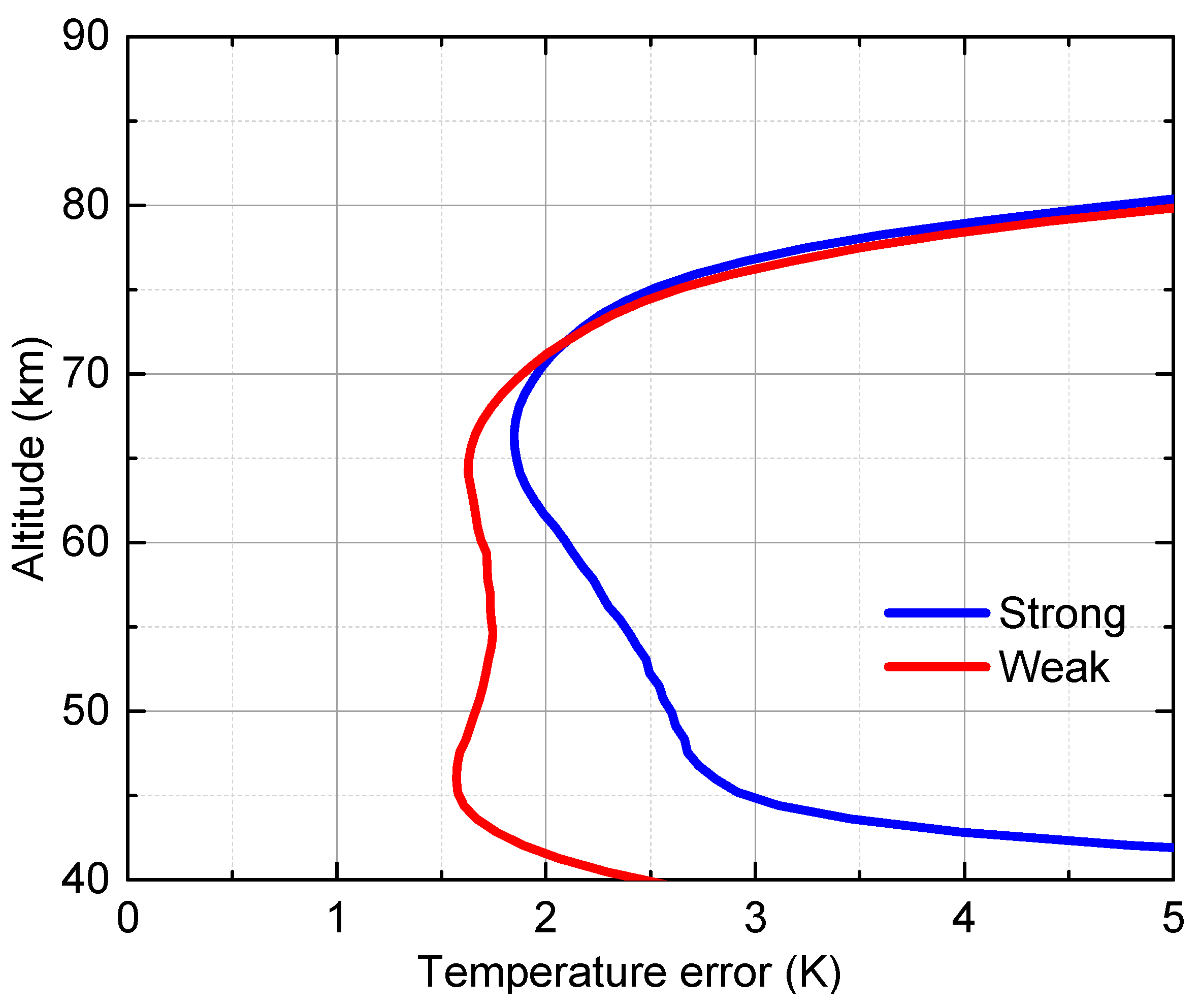Resulting from the attenuation of the O₂(a¹Δ_g) state density due to collisional quenching at a low tangent height, the limb-view weight comes down with the tangent height reduction, which causes a decrease in the measurement precision at low altitudes. The NWTSI wind and temperature error levels are quantified. The simulated results indicate a wind measurement precision of 1 to 3 m/s and a temperature precision of 1 to 3 K with horizontal resolutions of about 350 km along the line-of-sight and 170 km along the track over an altitude range from 40 km to 80 km, which meets the observing requirement in measurement precision for near-space detection. The NWTSI has the capability to address the link between dynamics and thermodynamics from the stratosphere to the mesosphere and could meet the need for global accurate and simultaneous observations of temperature and wind in the near space.