A Personalized Learning Path Problem Based on the Cognitive Theory of Multimedia Learning

Abstract

Educators increasingly rely on e-learning to supplement traditional classroom learning. Personalized learning paths (PLPs) have emerged as one type of supplement. A PLP is a sequence of learning materials (LMs) and activities that are selected according to LM fitness for the learner’s preferences and ordered according to prerequisite relationships. A problem that consistently emerges in PLP research is the use of pseudo-scientific learning theories to inform PLP design. This research presents LM and PLP rubrics, derived from the Cognitive Theory of Multimedia Learning (an experimentally validated learning theory) as a foundation that informs the PLP design process. The LM and PLP rubrics are decomposed into two problem domains, which include selecting and sequencing LMs to create PLPs. These problem domains are supported by proofs of NP-completeness. Next, real-world data are presented and used to derive instances of these multi-objective problems, which are then solved using the Non-Dominated Sorting Genetic Algorithm, a simulated annealing algorithm, and a Random Hill Climber algorithm. These metaheuristics produce satisfactory results, with the rubric scores of 12 student profiles ranging from $3.19$ to $3.54$ on a four-point scale. The rubrics, data, and algorithms used in this paper are publicly available.

1. Introduction

E-learning is increasingly used to complement traditional classroom instruction and to meet the evolving needs of diverse learners. In the fall of 2022, approximately 10 million students took online classes in the United States, and close to 100% of universities offered some kind of online instruction (Genevieve et al., 2024). Furthermore, the value of the e-learning market was USD 399.3 billion in 2022 and is expected to increase by 14% between 2023 and 2032 (Wadhwani, 2023), demonstrating the continued importance of using e-learning to reach students. One common e-learning tool that provides education to both students and working professionals is learning paths (LPs). LPs are sequences of learning activities and learning materials (LMs) (media content that provides education) that are designed by subject matter experts to meet a set of learning objectives. Common LP providers include Coursera (Coursera Investor Relations, 2025), the Khan Learning Academy (Khan Academy, 2025), and the Digital University of the United States Department of the Air Force (Department of the Air Force, 2024). Such LP providers often make available a portfolio of LMs that is too large for students to navigate or review without the assistance of prepackaging or specialized tool support.

Unfortunately, LPs are often “one size fits all”, implying that they do not change based on individual learner characteristics (A. Li et al., 2026; Nabizadeh et al., 2020). This lack of personalization impacts learners with unique time constraints or learning objectives. Such learners may not be able to find LPs that meet their specific needs. Researchers sometimes address this limitation of LPs by turning to personalized learning paths (PLPs) to provide tailored education to learners. PLPs are LPs that are designed specifically for a learner’s unique characteristics and constraints and are created on-demand using algorithmic techniques and associated data structures. Researchers are sometimes interested in tying their PLPs to learning science principles to improve the likelihood that their PLPs improve student learning outcomes. To this end, prior PLP researchers have tended to use learning styles in an attempt to provide a solid learning science foundation to PLPs (A. Li et al., 2026; Muhammad et al., 2016; Nabizadeh et al., 2020; Niknam & Thulasiraman, 2020; Raj & Renumol, 2022a, 2022b). Unfortunately, learning styles lack empirical evidence and are largely regarded as a myth in the education and psychology communities (Hattie & O’Leary, 2025; Kirschner, 2017; Nacekivell, 2019; Nancekivell et al., 2020; Yan & Fralick, 2022). The prevalence of the use of learning styles in PLP research indicates the need for a more established learning theory to be used as a foundation. This article leverages Cognitive Theory of Multimedia Learning (CTML) (Mayer, 2024; Mayer & Fiorella, 2022) as an appropriate choice for this foundational learning theory.

CTML offers a set of science-based principles with a clear learning theory lineage, validated by numerous studies that offer information about which specific LMs are more likely to be effective for specific learners (Mayer & Fiorella, 2022). Furthermore, CTML provides a universal framework for evaluating the quality of LMs based on how the human mind processes information. Rather than matching LMs to a learner’s supposed style, this approach focuses on selecting and sequencing LMs that are inherently effective for most learners due to their cognitive design and that have metadata characteristics that make them more likely to help specific learners to meet their learning objectives. As such, CTML is a strong candidate for guiding the development of PLPs by ensuring that each LM included adheres to evidence-based design principles that support learning.

As a first step towards developing and measuring PLPs according to established learning theory principles, rubrics based primarily on CTML principles and PLP use cases are proposed that quantify the quality of LMs and PLPs. These rubrics are then used to inform the following actions.

• Define the PLP problem domains. The multi-objective LM selection and sequencing problem domains are presented, which are designed to satisfy the LM and PLP rubrics.
• Prove the computational complexity of the multi-objective LM selection and sequencing problem domains. Both problems are supported by proofs of NP-completeness.
• Use real-world LM, learner profile, and knowledge graph data to specify instances of the LM selection and sequencing problem domains.
• Present algorithms and fitness functions that solve instances of the multi-objective LM selection and sequencing problem domains.
• Analyze the quality of the returned PLPs based on the LM and PLP rubrics.

These actions support the objective of presenting an example of translating a scientifically validated learning theory into a multi-objective PLP problem (a call to arms for future best practice). Additionally, these actions satisfy the following research questions:

• How can the PLP problem be defined in general, what are its relevant metrics, and which characteristics of CTML make it uniquely suited to the PLP problem? (Section 2)
• What are the formal definitions of the LM selection and sequencing problems, what can be proven about their computational complexities, which algorithms can be designed to solve multi-objective instantiations of these problems, and what are the experiments that can exercise these algorithms? (Section 3)
• What are the results of these experiments and what do they tell us about PLP design and the paradigms of the LM selection and sequencing problems? (Section 4)
• What are the implications of these experiments for the educational field and their limitations? (Section 5)

Finally, Section 6 is the conclusion and summarizes the results of this paper.

2. Background and Related Work

This section synthesizes the state of the art in PLP research to provide context for the proposed approach. Section 2.1 analyzes how the PLP problem is formally defined and structured in the literature. Section 2.2 evaluates the metrics commonly used with PLP approaches. Finally, Section 2.3 provides a foundational overview of CTML to facilitate the construction of the novel problems and metrics that are formally defined in Section 3.1.

2.1. The PLP Problem in the Literature

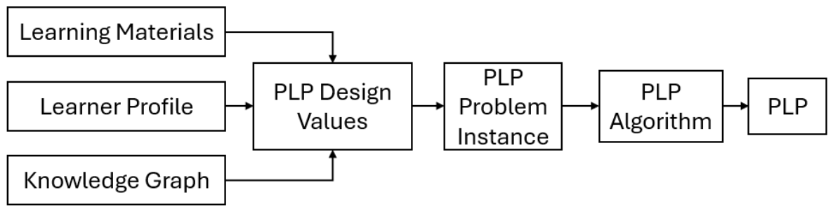
The PLP problem generally refers to the task of selecting and sequencing a subset of LMs to assist each learner in achieving their individual learning objectives. Figure 1 shows our outline of how PLPs are typically constructed. The use of a learning theory to inform the PLP design process is notably missing from Figure 1.

The first task of implementing the PLP problem framework is to define the computational PLP problems that need to be solved and the underlying LM metadata, learner profile, and knowledge graph that are used to populate these problem instances. Researchers take many approaches to this problem (Machado et al., 2021; Martins et al., 2021; Muhammad et al., 2016; Nabizadeh et al., 2020), but they generally use some kind of knowledge graph that describes the prerequisite relationships among KNs (“knowledge node” is synonymous with “topic”), along with a learner profile that includes a description of the learning objectives, preferred LM media content, learner cognitive levels for the KNs in the knowledge structure, and a metadata description of a corpus of LMs.

The PLP design variables are used to populate the specific PLP problem instances. Once a PLP problem instance is created, an algorithm is used to solve it. Prior examples of algorithmic approaches to PLP problems include exhaustive depth-first search, enumerating possible PLPs and returning the PLP that is the best fit for the student (Nabizadeh et al., 2020; Shi et al., 2020), and evolutionary algorithms or other metaheuristics, coupled with fitness functions exploring the search space for near-optimal PLPs (Benmesbah et al., 2023; C.-L. Bian et al., 2019; Pushpa, 2012; Vanitha & Krishnan, 2019; Zheng et al., 2025).

The appropriateness of the algorithmic approach varies based on the specific PLP problem variation. Depth-first search approaches have the advantage of being guaranteed to return a globally optimal solution. The approaches used in the two cited papers enumerate the entire search space without using any specific search heuristics, which may not scale depending on the structure of the knowledge graph and the relationship of the LMs and KNs (the authors did not report an excessive amount of time required in solving the PLP problem for the students in their studies) (Nabizadeh et al., 2020; Shi et al., 2020). Approaches using evolutionary algorithms or other metaheuristics have the advantage of superior scaling as NP-complete PLP problems become large, but they have a disadvantage in that they are not guaranteed to return globally optimal solutions. In these cases, the authors include metrics to argue that their approaches return satisfactory answers consistently based on their available data (Benmesbah et al., 2023; C.-L. Bian et al., 2019; Pushpa, 2012; Vanitha & Krishnan, 2019).

Finally, researchers might decompose the PLP problem into the separate problems of selecting and sequencing LMs, rather than both selecting and sequencing LMs in a single step (Kozierkiewicz-Hetmańska & Nguyen, 2011; Zhao et al., 2016; Zheng et al., 2023). This approach of dividing PLP problems into selection and sequencing has the advantage that these two problems are more tractable individually than in their combined form (although each sub-problem may still be NP-complete).

2.2. Common PLP Metrics Used in the Literature

The problem of defining which LMs help students to meet their learning objectives (and which LMs do not) is an important concept when discussing PLP metrics. This problem is equivalent to modeling the “real world” and reducing it to a problem domain that an algorithm can solve. This section reviews some of the most common metrics that are used to model learning path instructional design in the context of PLP problem instances. In PLP problems, researchers often assign LMs to “cover” KNs as a way to identify a subset of LMs that help students to meet their learning objectives (Chang & Ke, 2013; Gomez-Gonzalez & Jurado, 2012; H. Li et al., 2023; Machado et al., 2021; Mochocki et al., 2025; Nabizadeh et al., 2020; Son et al., 2021; Wang & Fu, 2021). In the context of LMs and KNs, when LM A covers KN B, this implies that LM A satisfies the learning objective captured by KN B.

This idea of coverage allows for additional metrics that attempt to discriminate between LMs on the basis of how well they help students to meet their learning objectives. Two common PLP problem metrics that rely on coverage are the average topic coverage and topic balance (Chang & Ke, 2013; Gomez-Gonzalez & Jurado, 2012; Machado et al., 2021; Wang & Fu, 2021). These metrics assume a many-to-many relationship between LMs and KNs, where one LM has the capacity to cover multiple KNs and one KN can be covered by multiple LMs. The average topic coverage rewards LMs for covering as many KNs as possible that are learner goals and not covering KNs that are not learner goals. Topic balance incentivizes LMs to cover learner goal KNs evenly (i.e., avoiding the situation wherein multiple LMs cover one KN and only one LM covers another).

PLP problems can also be many-to-one, where each LM covers only one KN but each KN can be covered by multiple LMs (Benmesbah et al., 2021, 2023; Mochocki et al., 2025; Nabizadeh et al., 2020). Finally, PLP problems can be one-to-one, where there is a one-to-one correspondence between LMs and KNs (Abu-Rasheed et al., 2023; Mochocki et al., 2025; Nabizadeh et al., 2017). The choice of many-to-many, many-to-one, or one-to-one models has significant implications for PLP design, as this choice can impact the appropriateness and utility of various PLP metrics and the algorithmic approach to solving PLP problem instances. For instance, the average topic coverage metric is not useful in many-to-one or one-to-one PLP problems as it does not discriminate between LMs that cover the learner’s target topics.

The many-to-many relationship between LMs and KNs implies greater computational difficulty and is often enough to take a PTIME problem and make it NP-complete (Mochocki et al., 2025). In a general many-to-many PLP problem, LMs may exist that cover one or more goal KNs and also cover one or more non-goal KNs, and some KNs may be covered by many LMs while some KNs may be covered by very few LMs. In these cases, researchers may have the aims of including LMs that cover the goal KNs, not including LMs that cover non-goal KNs, and including an even distribution of LMs across all goal KNs. In contrast, in many-to-one PLPs problems, each LM will only cover one KN, so an algorithm could easily prune LMs covering non-goal KNs from the search space before solving the problem. Additionally, algorithms could independently consider situations where one LM is allowed per KN or two LMs are allowed per KN, etc., such that perfect topic balance is guaranteed. Therefore, the average topic coverage and topic balance are metrics that are specifically introduced in many-to-many PLP problems to address the added complexity of the many-to-many relationship, and they are not necessary in many-to-one or one-to-one PLP problems (as simpler heuristics are available that accomplish the same goals).

While many-to-many PLP problems introduce increased difficulty computationally, in terms of both selecting and sequencing LMs, they have the advantage that they are easier to identify and curate. For instance, let us consider a university lecture that covers multiple topics. Unless effort is devoted to breaking the video down into segments that correspond to specific KNs, such a video is likely to be many-to-many as it will cover a range of KNs. Therefore, if a PLP approach is to take a large set of open-source LMs, the problem is likely to be many-to-many unless they are broken down into smaller pieces (a many-to-one construction). So, the tradeoff is that many-to-many PLP problems are more difficult computationally but require less preprocessing, while many-to-one PLP problems are easier computationally but require more preprocessing. Additionally, according to the segmenting principle from CTML, there may also be an advantage in breaking LMs into smaller components that are easier for students to understand.

Table 1. This table provides common examples of many-to-many, many-to-one, and one-to-one PLP problems, along with advantages and disadvantages of each. A recent publication detailing an integrated PLP framework assumes a many-to-many relationship (Zheng et al., 2025).

	Many-to-Many	Many-to-One	One-to-One
LM Mapping	Covers many KNs	Covers exactly 1 KN	Covers exactly 1 KN
KN Mapping	Covered by many LMs	Covered by many LMs	Covered by exactly 1 LM
Common Example	A knowledge graph is designed on a general topic and open-source LMs are collected that provide education on KNs in this knowledge graph. An example of an LM is a university lecture that covers multiple KNs.	A university professor identifies the relevant KNs in one of their courses and organizes them into a knowledge graph based on prerequisite relationships. The professor curates beginning and advanced LM “chunks” for each KN.	A university professor takes the LMs from their course and organizes them into a graph indicating prerequisite relationships between LMs.
Advantages	Less preprocessing. Open-source LMs are likely to be many-to-many and can be pulled directly into PLP problems with minimal effort.	Computationally less expensive. Many-to-one PLP problems are often PTIME, where many-to-many PLP problems would be NP-complete (Mochocki et al., 2025).	Normal approach when university courses are mapped directly to PLP problems. Instructors will take the existing corpus of LMs and organize them into a graph where the edges indicate the sequence of study.
Disadvantages	Computationally more expensive. Many-to-many LMs often make PTIME PLP problems NP-complete (Mochocki et al., 2025).	More preprocessing. Open-source LMs may require chunking before inclusion in PLP problems.	One-to-one PLPs do not scale well with a large number of LMs. Some personalization options become harder, such as providing students LMs that are of an appropriate difficulty level.

describes some of the characteristics of each approach in more detail.

Along with those related to KN coverage, PLP researchers use additional metrics to measure the quality of a PLP for a given learner. Two of the most common metrics used by researchers are the difficulty of the LM in comparison to the learner’s cognitive level and the sum of LM durations in comparison to the learner’s time constraints (Machado et al., 2021; Mochocki et al., 2025; Muhammad et al., 2016; Nabizadeh et al., 2020). Furthermore, many researchers attempt to match LMs to learners on the basis of learning styles (Machado et al., 2021; Muhammad et al., 2016; Nabizadeh et al., 2020), media preference matching (Mochocki et al., 2025; Muhammad et al., 2016; Nabizadeh et al., 2020), or the “distance” between LMs and the KNs that they cover (Acampora et al., 2011) (where a greater distance implies that an LM covers a topic less adequately). Meanwhile, other PLP approaches include maximizing LM “cohesiveness” (Hnida et al., 2018) (how well they work together to provide education) or minimizing the lack of LM cohesiveness (the degree to which LMs negatively impact learning when they appear together in a PLP) (C. Bian et al., 2017; C.-L. Bian et al., 2019; Wan & Niu, 2016).

Some of these metrics are justifiable by learning science principles or by realistic use cases. For instance, the matching of LMs to learners based on difficulty and KN cognitive levels aligns with the assumption of the limited nature of working memory in CTML (Mayer & Fiorella, 2022). Examples of common PLP use cases are when a learner has a tight time constraint for their learning path (necessitating the time constraint metric), when they prefer LMs that are audio-only due to aligning PLP completion with their daily exercise routines, and when they prefer them to be silent so as not to be disruptive in a work environment.

2.3. CTML Overview

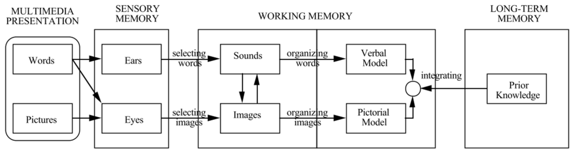
CTML offers scientifically supported principles that are suitable as a foundation for PLP design. These principles are based on the goals of minimizing extraneous cognitive processing (i.e., not requiring students to use limited capacity for unessential information), managing essential processing (assisting with schema development in working memory), and fostering generative processing (assisting with understanding information) (Mayer & Fiorella, 2022). Additionally, CTML has the assumptions that humans have dual channels (their ears and eyes) and a limited capacity for information processing in their working memory and that active processing is necessary to develop schemata in long-term memory (Mayer, 2024). Figure 2 illustrates the Cognitive Theory of Multimedia Learning.

CTML leans heavily on Cognitive Load Theory (Mutlu-Bayraktar et al., 2019) when stressing the importance of managing a student’s cognitive load (Mayer & Fiorella, 2022). Management of this load can be traced to providing students LMs at an appropriate difficulty level and to ranking LMs more highly when they are compliant with CTML principle best practices. To this end, two rubrics (the LM rubric and the PLP rubric) are used to assist in personalizing PLPs for students. The LM rubric quantitatively measures LM compliance with CTML principles. The data package accompanying this article includes an assessment of 365 LMs (labeled using the LM rubric) on a scale of 1–4, where 4 indicates compliance, 1 indicates a lack of compliance, and 2 and 3 indicate varying degrees of compliance. The four-point scale both avoids a neutral value and allows users to estimate LM compliance with CTML principles without suggesting the artificial precision that larger scales might. Human researchers used this scale to rate the 365 LMs used in Section 3.

The LM rubric describes the 12 CTML principles and how LMs are measured based on these principles according to the Likert-style compliance categories. These principles include the following (with definitions provided from the Cambridge Handbook of Multimedia Learning (Mayer & Fiorella, 2022)):

• Multimedia Principle: “People learn better from words and pictures than from words alone.”
• Coherence Principle: “People learn better when extraneous material is excluded rather than included.”
• Worked Example Principle: “Learners gain deep understanding in multimedia learning environments when they receive worked examples in initial cognitive skills acquisition.”
• Segmenting Principle: “People learn better when a multimedia lesson is presented in user-paced segments rather than as a continuous unit.”
• Signaling Principle: “People learn better when cues are added that highlight the organization of the essential material.”
• Spatial Contiguity Principle: “People learn better when corresponding words and pictures are presented near rather than far from each other on the page or screen.”
• Temporal Contiguity Principle: “People learn better when corresponding words and pictures are presented simultaneously rather than successively.”
• Modality Principle: “People learn better from graphics and narration than from graphics and on-screen text.”
• Redundancy Principle: “People do not learn better when printed text is added to graphics and narration; people learn better from graphics and narration than from graphics, narration, and printed text, when the lesson is fast paced.”
• Personalization Principle: “People learn better from multimedia lessons when words are in conversational style rather than formal style.”
• Voice Principle: “People learn better when the narration in multimedia lessons is spoken in a friendly human voice rather than a machine voice.”
• Sourcing Principle: “Taking the source of a document into account contributes to a learner’s deep understanding of the document.”

These principles have been validated through scientific testing with numerous studies and varying effect sizes (Mayer, 2024). For instance, a study from 2020 demonstrated that, when videos are reduced to smaller sizes, students’ cognitive load was reduced and learning improved (Altinpulluk et al., 2020), further validating the segmenting principle. A subset of these principles was also used to inform the PLP rubric design, which is the foundation of the PLP design process. For the theoretical background and descriptions of these principles, review the rubrics and Mayer’s seminal work on CTML (Mayer & Fiorella, 2022).

3. Materials and Methods

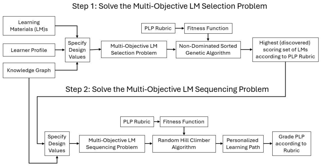
This section introduces the formal definitions of the PLP problems and their computational complexity, explains how data are used to create instances of these problems, and describes the algorithms used to solve these problem instances. The overall methodology is generally based on the Design Science Research Process for Information Systems (Peffers et al., 2007). The specific methodological steps are mapped against the Design Science Research steps in

Table 2. This table maps the Design Science Research stages to the PLP research methodology employed in this paper (Peffers et al., 2007). The central idea is to start with the scientifically validated learning theory and use this to inform the remainder of the work. Human experiments are missing from this table and should be included in the evaluation stage in future work.

DSR Stage (Peffers et al., 2007)	PLP Research Methodology	Section	Explanation
1. Problem identification and motivation	Identify a scientifically validated learning theory as a basis for the PLP approach	Section 2.3	Current PLP approaches tend to not start with scientifically validated learning theories
2. Define the objectives for a solution	Design a way to quantitatively rank PLPs based on the learning theory (LM and PLP rubrics)	Section 3.1	There is currently no standard for quantitatively measuring the quality of PLPs
	Formally define the PLP problem		Formally defining the PLP problem facilitates the development of an algorithmic solution
	Prove the computational complexity of the PLP problem and its relevant variations		Proving the computational complexity of a problem assists with choosing algorithms that are a fit for the problem
3. Design and development	Use real-world data to create instances of the problem domain	Section 3.2	Real-world data allow the design of an experiment to exercise the problem definition
	Design algorithms to solve these real-world instances	Section 3.3	Algorithms are necessary to return solutions to real-world problem instances
4. Demonstration	Run experiments and return PLPs quantitatively measured by rubrics	Section 4	Once designed, the algorithms need to be tested
5. Evaluation	Run statistical tests to validate experiments		Statistical tests ensure that the algorithms are performing within anticipated parameters
	Analyze the results of the experiment and compare these results to what was expected based on available data and proofs of computational complexity		The experimental results should be explainable based on the proofs of computational complexity and through the unique characteristics of the data
6. Communication	Analyze lessons learned from the methodology	Section 5 and Section 6	Lessons learned from the methodology should be analyzed so that improvements can be made in the future
	Discuss limitations of the work and recommend future directions		Best practice for research papers

. Figure 3 shows the overall methodology of this approach, including the specific algorithms used to solve the LM selection and sequencing problems.

3.1. PLP Problem Design and Complexity Analysis

The two-part PLP problem domain is derived from the PLP and LM rubrics. This problem is decomposed into two activities: LM selection and LM sequencing. The LM selection problem uses principles that are derived from CTML. These problems are designed so that solutions that satisfy the decision problems would also score well according to the PLP rubric. In this section, we provide an overview of the rubrics and their design, before formally defining the multi-objective selection and sequencing problems.

The relevant PLP rubric categories are presented, before formally defining the multi-objective LM selection problem.

Table 3. Justification for objectives in the LM selection problem based on CTML theory and PLP research.

Objective	Var.	Justification and Sources
Learner CTML Value	$V_p$	Combination of LM CTML compliance categories. (Mayer & Fiorella, 2022)
Learner Difficulty Matching	$D_p$	Limited working memory of learners. (Mayer & Fiorella, 2022; Mutlu-Bayraktar et al., 2019)
Learner Preference Value	$O_p$	Learners may prefer specific LM format. (Mochocki et al., 2025; Muhammad et al., 2016; Nabizadeh et al., 2020)
Time Interval Constraint	$T_p$	Learners may have time constraints. (Machado et al., 2021; Mochocki et al., 2025; Muhammad et al., 2016; Nabizadeh et al., 2020)
LM Cohesiveness	$E_p$	Standardizing terminology between LMs may help beginning learners. (Mayer & Fiorella, 2022)
LM Coherence	$C_p$	Students should not be provided LMs that cover non-goal KNs. (Mayer & Fiorella, 2022)
Segmenting Principle	$S_p$	Providing more targeted LMs may help learners. (Mayer & Fiorella, 2022)
Multi-Doc Integration	$M_p$	Providing multiple LMs on the same topic may help students to learn more deeply. (Mayer & Fiorella, 2022)
Topic Balance	$B_p$	Provides learners with a balanced education across topics. (Chang & Ke, 2013; Gomez-Gonzalez & Jurado, 2012; Machado et al., 2021; Wang & Fu, 2021)

justifies the LM selection objectives on the basis of a foundational learning theory or the PLP literature.

Table 4. A summary of the variables and rubric categories that are used in the multi-objective LM selection problem to score a candidate solution p.

Rubric Category	Problem Values (p Indicates Score of Candidate PLP)	(4) Compliant	(3) Mostly Compliant	(2) Partially Compliant	(1) Not Compliant
CTML Principle Matching	$V_p\in [1,4]$	$V_p\ge 3.25$	$2.5\le V_p<3.25$	$1.75\le V_p<2.5$	$V_p<1.75$
LM Difficulty Matching	$D_p\in [0,1]$	$D_p\ge 0.75$	$0.5\le D_p<0.75$	$0.25\le D_p<0.5$	$D_p<0.25$
Learner Preference Matching	$O_p\in [0,1]$	$O_p\ge 0.75$	$0.5\le O_p<0.75$	$0.25\le O_p<0.5$	$O_p<0.25$
Time Interval Constraint	Lower bound: $T_L\ge 0$ Upper bound: $T_U\ge T_L$ PLP duration: $T_p\ge 0$	$T_L\le T_p\le T_U$	$0.9T_L\le T_p<T_L$ ∨ $T_U<T_p\le 1.1T_U$	$0.8T_L\le T_p<0.9T_L$ ∨ $1.1T_U<T_p\le 1.2T_U$	$T_p<0.8T_L$ ∨ $T_p>1.2T_U$
LM Cohesiveness	$E_p\in [0,1]$	$E_p\ge 0.75$	$0.5\le E_p<0.75$	$0.25\le E_p<0.5$	$E_p<0.25$
Coherence	$C_p\ge 0$	$C_p\le 0.25$	$0.25<C_p\le 0.5$	$0.5<C_p\le 1.0$	$C_p>1.0$
Segmenting	$S_p\ge 1$	$S_p\le 2$	$2<S_p\le 3$	$3<S_p\le 4$	$S_p>4$
Multiple-Document Integration Principle	$M_p\ge 0$	$M_p\ge 4$	$3\le M_p<4$	$2\le M_p<3$	$M_p<2$
Topic Balance	$B_p\ge 0$	$B_p\le 0.3$	$0.3<B_p\le 0.5$	$0.5<B_p\le 0.7$	$B_p>0.7$

informs the LM selection decision problem (e.g., does a PLP exist such that it scores 3 in all categories?).

3.1.1. Multi-Objective LM Selection Decision Problem

In the multi-objective LM selection decision problem, we are given a set of LMs $L=\{{\ell }_1,{\ell }_2,\dots ,{\ell }_n\}$. With each $j\in \{1,2,\dots ,n\}$, four parameters are associated with the LM ${\ell }_j$, namely the difficulty matching value $d_j\in [0,1]$, the CTML value $v_j\in [1,4]$, the learner preference value $o_j\in [0,1]$, and the duration $t_j\ge 0$. Also given are the sets of KNs $K=\{k_1,k_2,\dots ,k_m\}$ and the function $f:L\times K\to \{0,1\}$ that describes the many-to-many relationship between the KNs and the LMs, where $f(\ell ,k)=1$ exactly when ℓ covers k, and the cohesiveness function $E:L\times L\to [0,1]$. Also given is the learner difficulty matching goal $D\in [0,1]$; the learner CTML goal $V\in [1,4]$; the learner preference goal $O\in [0,1]$; the time interval goals $T_L$ and $T_U$, where $0\le T_L\le T_U$; the balance goal B; the multiple-document integration goal M; the coherence goal C; the segmenting goal S; and the cohesiveness goal E.

We define the subset of KNs $g\subseteq K$ as the set of KNs to be covered (thereby modeling the learner’s goals). The PLP $p\subseteq L$ has the decision variables ${\chi }_j\in \{0,1\}$ by ${\chi }_j=1$ if ${\ell }_j\in p$, while ${\chi }_j=0$ otherwise.

Such a PLP has the following values.

• Learner CTML Value:

  $$V_p={\displaystyle \frac{{\sum }_{j=1}^n{\chi }_j{v}_j}{\left|p\right|}}$$
• Learner Difficulty Matching Value:

  $$D_p={\displaystyle \frac{{\sum }_{j=1}^n{\chi }_j{d}_j}{\left|p\right|}}$$
• Learner Preference Value:

  $$O_p={\displaystyle \frac{{\sum }_{j=1}^n{\chi }_j{o}_j}{\left|p\right|}}$$
• Duration: $T_p={\sum }_{j=1}^n{\chi }_j{t}_j$.
• LM Cohesiveness Value:

  $$E_p={\displaystyle \frac{{\sum }_{i=1}^{n-1}{\sum }_{j=i+1}^n{\chi }_i{\chi }_{j}E({\ell }_i,{\ell }_j)}{\frac{1}{2}\left(\right|p\left|\right)\left(\right|p|-1)}}$$
• Coherence Principle Value:

  $$C_p={\displaystyle \frac{{\sum }_{k\notin g}{\sum }_{j=1}^n{\chi }_{j}f({\ell }_j,k)}{\left|p\right|}}$$
• Segmenting Principle Value:

  $$S_p={\displaystyle \frac{{\sum }_{i=1}^m{\sum }_{j=1}^n{\chi }_{j}f({\ell }_j,k_m)}{\left|p\right|}}$$
• Multiple-Document Integration Principle Value:

  $$M_p={\displaystyle \frac{{\sum }_{k\in g}{\sum }_{j=1}^n{\chi }_{j}f({\ell }_j,k)}{\left|g\right|}}$$
• Balance Cover Value: Relative Standard Deviation

  $$B_p={\displaystyle \frac{\sqrt{\frac{{\sum }_{k\in g}{\left({\sum }_{j=1}^n{\chi }_{j}f({\ell }_j,k)-\frac{{\sum }_{f=1}^n{\sum }_{k\in g}{\chi }_{f}f({\ell }_f,k)}{\left|g\right|}\right)}^2}{\left|g\right|}}}{\frac{{\sum }_{f=1}^n{\sum }_{k\in g}{\chi }_{f}f({\ell }_f,k)}{\left|g\right|}}}$$

The question to be answered is whether there exists a PLP such that $V_p\ge V$, $D_p\ge D$, $O_p\ge O$, $T_L\le T_p\le T_U$, $E_p\ge E$, $C_p\le C$, $S_p\le S$, $M_p\ge M$, and $B_p\le B$.

3.1.2. Multi-Objective LM Selection Problem Is in NP

Consider the following polynomial-time algorithm that verifies that a solution to the multi-objective LM selection problem satisfies its constraints. Consider a candidate PLP p and a knowledge set g.

• Return false if $V_p<V$.
• Return false if $D_p<D$.
• Return false if $O_p<O$.
• Return false if $T_p<T_L$ or $T_p>T_U$.
• Return false if $E_p<E$.
• Return false if $C_p>C$.
• Return false if $S_p>S$.
• Return false if $M_p<M$.
• Return false if $B_p>B$.
• Return true.

This reduction runs in $O(mn+n^2)$, meaning that the multi-objective LM selection problem is in NP.

3.1.3. Multi-Objective LM Selection Problem Is NP-Complete

The following is a polynomial-time (PTIME) reduction of the Subset Sum problem (Karp, 1972) to the multi-objective LM selection problem using only the time interval objective. In the Subset Sum problem, we are given the set of non-negative integers $S=\{s_0,s_1,\dots ,s_n\}$, each with decision variable ${\chi }_j$ and the goal value W. The question to be answered is whether a subset of integers exists such that ${\sum }_{j=1}^n{\chi }_j=W$. Given an arbitrary instance of the Subset Sum problem, consider the following algorithm that reduces it to the multi-objective LM selection problem in polynomial time.

• For each integer $s_j\in S$, create an LM ${\ell }_j\in L$. Set $t_j=s_j$.
• Set $T_L=T_U=W$.
• Create KN k and $\forall L$; assign $f(\ell ,k)=1$ and set $g=k$.
• $\forall L$, assign $v_j=4,d_j=1,o_j=1$.
• $\forall {\ell }_i,{\ell }_j\in L$, where $i\ne j$, and set $E({\ell }_i,{\ell }_j)=1$.
• Set $V=0,D=0,O=0,E=0,C=1,S=1,M=0$, and $B=1$.

This algorithm takes place in $O\left(n\right)$ time. The main step of this reduction is setting $T_L=T_U=W$. Therefore, for the LM selection problem to have a ‘yes’ decision, there must be a subset of LMs such that $T_p=T_L=T_U=W$. Recall that the decision problem in the LM selection problem is whether there exists a subset of LMs such that $T_L\le T_p\le T_U$ (along with other constraints that are automatically satisfied by the construction above). Therefore, when $T_L=T_U$, the only valid solutions have $T_p=T_L=T_U$. A subset of LMs with this property corresponds to a subset of integers in S satisfying the Subset Sum instance. Thus, there exists a solution to the multi-objective LM selection problem instance if and only if there is also a solution to the Subset Sum problem instance. Because the NP-complete Subset Sum problem can be reduced in polynomial time to the multi-objective LM selection problem, the latter is NP-hard. As noted above, it is also in NP, so it is NP-complete.

This proof demonstrates that the multi-objective LM selection problem is NP-complete even when only considering the time interval requirement. Future work includes proving that various other elements of the problem are also sufficient for NP-completeness.

3.1.4. Deriving the Multi-Objective LM Sequencing Problem

After selecting LMs, the next step is to sequence them so that the learner has the best opportunity to understand the content of the underlying KNs. This section presents an analysis of a problem domain that integrates three elements: elaboration, difficulty, and interleaving. These categories are derived from scientifically validated learning theory best practices (Carey, 2015; Morrison et al., 2019). The rubric scores for these three categories are defined based on compliance and indicate the percentage range of possible violations that occurred as follows: 4 (fewer than 25%), 3 (at least 25% and fewer than 50%), 2 (at least 50% and fewer than 75%), and 1 (at least 75%).

• Elaboration: When LMs are organized according to elaboration, LMs that cover more general KNs are placed before LMs that cover more specific KNs. This allows learners to develop an understanding of general topics before being exposed to specific topics (Morrison et al., 2019). The prerequisites in the multi-objective LM sequencing problem are derived from these elaboration relationships.
• Difficulty: When LMs are organized according to difficulty, easier LMs are placed before more difficult LMs (Morrison et al., 2019). This helps learners to develop basic scaffolding for less difficult LMs before being exposed to more difficult LMs.
• Interleaving: When LMs are interleaved, consecutive LMs do not cover the same KNs (Carey, 2015). This objective models interleaved practice, where learners alternate in practicing related skills in order to achieve deeper comprehension of how they relate.

This section proposes an NP-complete multi-objective problem for which the task is to sequence a set of LMs satisfying the multi-objective LM selection decision problem (Section 3.1.1) according to these three sequencing approaches. As with the LM selection problem, the LMs are assumed to have a many-to-many relationship with the KNs. As will be shown, this many-to-many relationship is by itself sufficient for the sequencing problem to be NP-complete in the cases of either interleaving or prerequisite sequencing. A summary of the proofs in this section is provided in

Table 5. Summary of computational complexity for the multi-objective PLP sequencing problem. The objectives are interleaving (I), prerequisite sequencing (P), and difficulty sequencing (D). Complexities marked with an * indicate original proofs in this paper. All graphs are assumed to be directed acyclic graphs (DAGs), and the LMs have a many-to-many coverage relationship with the KNs.

I	P	D	Complexity	Justification
X	X	X	NP-complete *	Combined NP-hard problem proven to be in NP
X			NP-complete *	Reduction from Hamiltonian Path
	X		NP-complete *	Reduction from Minimum Feedback Arc
		X	PTIME	Sorting algorithm

and

Table 6. Summary of computational complexity for the many-to-one PLP sequencing problem. The objectives are interleaving (I), prerequisite sequencing (P), and difficulty sequencing (D). Computational complexities marked with an * indicate original proofs in this paper. All graphs are assumed to be DAGs.

I	P	D	Complexity	Justification
X	X	X	Unknown	Future work
X			PTIME *	Polynomial-time algorithm proven to be globally optimal solution
	X		PTIME	Topological sort returns globally optimal solution
		X	PTIME	Sorting algorithm

.

3.1.5. Multi-Objective LM Sequencing Problem

In the multi-objective LM sequencing problem, we are given a set of LMs $L=\{{\ell }_1,{\ell }_2,\dots ,{\ell }_n\}$. Each $i\in \{1,2,\dots ,n\}$ is associated with difficulty $h_i$ of the LM ${\ell }_i$. Also given is the directed acyclic graph $G=(K,E)$, where the set of KNs is $K=\{k_1,k_2,\dots ,k_m\}$ and $E\subseteq K\times K$, where $(k_u,k_v)\in E$ indicates that $k_u$ is a prerequisite of $k_v$.

We also have a set of $n^2$ decision variables ${\chi }_{ij}\in \{0,1\}$ that describes the sequence of LMs where, for $i,j\in \{1,2,\dots ,n\}$, ${\chi }_{ij}=1$ exactly when LM ${\ell }_i$ is located in position j. A candidate PLP is a valid assignment of these decision variables according to the following constraints:

• Each LM in a PLP must occupy exactly one index ($\forall i{\sum }_{j=1}^n{\chi }_{ij}=1$).
• Each sequence element in a PLP must be occupied by exactly one LM ($\forall j{\sum }_{i=1}^n{\chi }_{ij}=1$).

We also define the following functions to support discriminating between PLPs:

• The function $f:L\times K\to \{0,1\}$ that describes the many-to-many coverage of the KNs by the LMs, where $f(\ell ,k)=1$ when ℓ covers k and $f(\ell ,k)=0$ otherwise.
• The difficulty scoring function $D:L\times L\to \{0,1\}$, where $D({\ell }_x,{\ell }_y)=1$ when $h_x>h_y$ and $D({\ell }_x,{\ell }_y)=0$ when $h_x\le h_y$.

A candidate PLP, p, has three scores. These are difficulty sequencing $H_p$, prerequisite sequencing $R_p$, and interleaving $I_p$. The multi-objective goal is to minimize each score.

The first score is $H_p$, which is calculated by counting the number of times that a more difficult LM is at a lower index than a lower-difficulty LM. This difficulty sequence score is calculated for p as follows:

$$H_p={\displaystyle \sum _{i=1}^{n-1}}{\displaystyle \sum _{x=i+1}^n}{\displaystyle \sum _{j=1}^{n-1}}{\displaystyle \sum _{y=j+1}^n}\left\{{\chi }_{ij}{\chi }_{xy}D({\ell }_i,{\ell }_x)+{\chi }_{xj}{\chi }_{iy}D({\ell }_x,{\ell }_i)\right\}$$

In calculating $H_p$, the summations iterate across all pairs of LMs $({\ell }_i,{\ell }_x)$ and pairs of indices $(j,y)$ and checks for the conditions where ${\ell }_i$ is at a lower index than ${\ell }_x$ (${\ell }_i$ is in index j, while ${\ell }_x$ is in index y) and that $h_i>h_x$, or that ${\ell }_x$ is at a lower index than ${\ell }_i$ (${\ell }_x$ is in index j, while ${\ell }_x$ is in index y) and that $h_x>h_i$. For the first pair of decision variables ${\chi }_{ij}{\chi }_{xy}$, their values are both 1 exactly when ${\ell }_i$ proceeds ${\ell }_x$ in the sequence; for the second pair of decision variables ${\chi }_{xj}{\chi }_{iy}$, their values are both 1 exactly when ${\ell }_x$ proceeds ${\ell }_i$ in the sequence.

The second score is the prerequisite sequencing score, $R_p$. This score is calculated by considering all edges and pairs of LMs in the sequence. We count those for which one LM covers the prerequisite KN, one LM covers the target KN, and the LM covering the target KN precedes the LM covering the prerequisite KN (the prerequisite constraint is violated). This score, $R_p$, is calculated for p as follows:

$$R_p=\sum _{(k_u,k_v)\in E}{\displaystyle \sum _{i=1}^{n-1}}{\displaystyle \sum _{x=i+1}^n}{\displaystyle \sum _{j=1}^{n-1}}{\displaystyle \sum _{y=j+1}^n}\left\{{\chi }_{ij}{\chi }_{xy}f({\ell }_i,k_v)f({\ell }_x,k_u)+{\chi }_{xj}{\chi }_{iy}f({\ell }_x,k_v)f({\ell }_i,k_u)\right\}$$

In calculating $R_p$, we consider each edge $(k_u,k_v)\in E$ and sum across all pairs of LMs $({\ell }_i,{\ell }_x)$ and pairs of indices $(j,y)$ to identify the cases for which either (1) ${\ell }_i$ precedes ${\ell }_x$ and $f({\ell }_i,k_v)=f({\ell }_x,k_u)=1$, or (2) ${\ell }_x$ precedes ${\ell }_i$ and $f({\ell }_x,k_v)=f({\ell }_i,k_u)=1$. Since $(k_u,k_v)\in E$, case (1) means that ${\ell }_x$ covers a KN that is a prerequisite for a KN covered by ${\ell }_i$, while case (2) means that ${\ell }_i$ covers a KN that is a prerequisite for a KN covered by ${\ell }_x$.

Finally, we have the interleaving score, $I_p$. This score is calculated by counting the pairs of adjacent LMs that cover the same KN (violating the interleaving constraint):

$$I_p={\displaystyle \sum _{i=1}^{n-1}}{\displaystyle \sum _{x=i+1}^n}{\displaystyle \sum _{j=1}^{n-1}}\left\{({\chi }_{ij}{\chi }_{x(j+1)}+{\chi }_{xj}{\chi }_{i(j+1)})\times {\displaystyle \sum _{c=1}^m}f({\ell }_i,k_c)f({\ell }_x,k_c)\right\}$$

In calculating $I_p$, we iterate across all pairs of LMs $({\ell }_i,{\ell }_x)$ and all pairs of adjacent positions j and $j+1$. ${\chi }_{ij}{\chi }_{x(j+1)}=1$ exactly when ${\ell }_i$ is in position j and ${\ell }_x$ is in position $j+1$, while ${\chi }_{xj}{\chi }_{i(j+1)}=1$ exactly when ${\ell }_x$ is in position j and ${\ell }_i$ is in position $j+1$. Whenever the LMs are adjacent in the sequence, we iterate over the set of KNs to check the condition that they both cover the same KN $k_c$.

We are also given the difficulty sequencing goal H, the prerequisite sequencing goal R, and the interleaving sequencing goal I. The question to be answered is whether a PLP p exists such that $H_p\le H$, $R_p\le R$, and $I_p\le I$.

The next few sections show that, based on this description, the multi-objective LM sequencing problem is in NP. They also show that the problem is NP-complete even when exclusively considering interleaving or prerequisite sequencing (even in the case of a DAG) but in PTIME when only considering difficulty scoring. Following these proofs, the paper explores the consequences of a many-to-one relationship between the LMs and KNs in these sequencing problem versions.

3.1.6. The Multi-Objective LM Sequencing Problem Is in NP

Consider the following polynomial-time algorithm that verifies that a solution to a multi-objective LM sequencing problem instance satisfies the constraints. Consider a candidate LM sequence p.

• Return false if $\forall i{\sum }_{j=1}^n{\chi }_{ij}\ne 1$.
• Return false if $\forall j{\sum }_{i=1}^n{\chi }_{ij}\ne 1$.
• Return false if $H>H_p$.
• Return false if $R>R_p$.
• Return false if $I>I_p$.
• Return true.

This certifier takes place in $O\left(n^4\right)$, confirming that this problem is in NP.

3.1.7. The Many-to-Many LM Interleaving Sequencing Problem Is NP-Complete

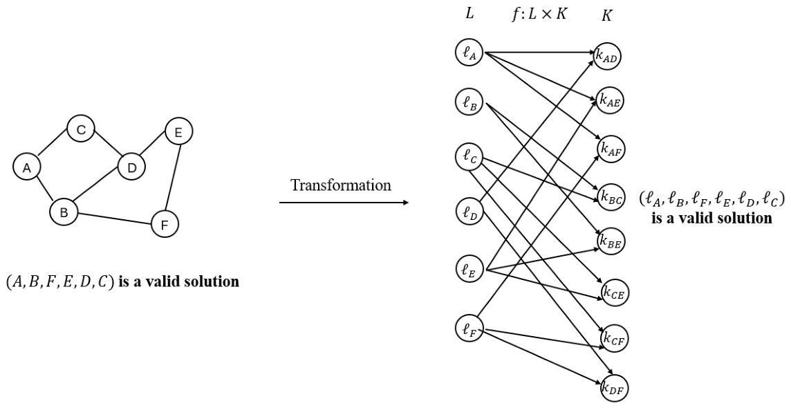
The following proof presents a polynomial-time reduction of the Hamiltonian Path problem Karp (1972) to the multi-objective LM sequencing problem using only the interleaving objective. In an instance of the Hamiltonian Path problem, we are given a graph $G(V,E)$, where V is a set of vertices and E is a set of edges, where each edge is a pair of vertices $(u,v)\in V\times V$. The question to be answered is whether there exists a path in G such that every vertex in V is visited exactly once. Given an arbitrary instance of the Hamiltonian Path problem, consider the following algorithm (graphically represented in Figure 4):

• $\forall v\in V$; create an LM $\ell \in L$. Set the difficulty of all LMs to 1.
• $\forall (u,v)\in V$ where $(u,v)\notin E$; create a KN $k\in K$ and assign $f({\ell }_u,k)=1$ and $f({\ell }_v,k)=1$.
• Set $I=0$, $R=0$, and $H=0$.

The runtime of this reduction is $O\left(\right|V{|}^2)$. We now have a set of LMs and KNs, where each LM represents a vertex from the Hamiltonian Path problem instance and the KNs complement the edges from the Hamiltonian Path problem instance. In other words, if two vertices are incident in the Hamiltonian Path problem instance, then their respective LMs do not cover any of the same KNs, while, if they are not incident, then their respective LMs both cover some KNs. The construction of the knowledge graph guarantees that it is acyclic, implying that the LM sequencing problem instance created by this polynomial-time algorithm is a valid instance of the multi-objective LM sequencing problem.

In this reduction, every KN is covered by exactly two LMs. The interleaving constraint being set to 0 implies that, given a solution, no LMs appearing consecutively in the sequence cover the same KN. Thus, the corresponding pair of vertices must be incident in the Hamiltonian Path problem instance. It follows that the sequence of LMs corresponds to a sequence of vertices satisfying the Hamiltonian Path problem instance. Therefore, the multi-objective LM sequencing problem is NP-hard, and, because it is in NP, it is NP-complete.

All of the LM difficulties are set to 1, which means that $H_p=0$ for all sequences. No edges are included between KNs (which would represent prerequisite relationships), so $R_p=0$ for all sequences. Therefore, this reduction relies exclusively on the interleaving constraint. The next section proves that the prerequisite sequencing problem is also NP-complete in the many-to-many case.

3.1.8. The Many-to-Many Prerequisite Sequencing Problem Is NP-Complete

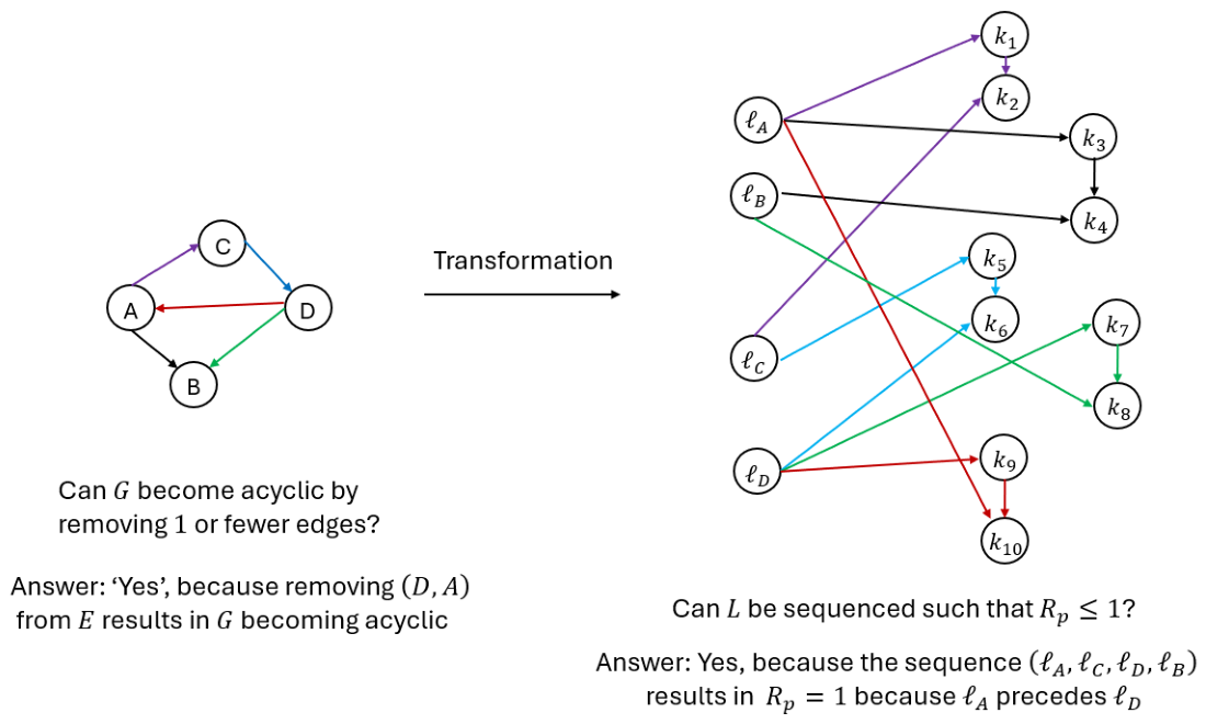
This section provides a polynomial-time reduction of the Minimum Feedback Arc problem (Karp, 1972) to the multi-objective LM sequencing problem using only the prerequisite objective. In the Minimum Feedback Arc problem, we are given a directed graph $G(V,E)$, where V is a set of vertices and E is a set of directed edges, where $(u,v)\in E$ is an edge from u to v. Graphs containing self-edges are excluded. Also given is the edge removal goal z. The question to be answered is whether z or fewer edges can be removed from E such that G becomes acyclic. Given an arbitrary instance of the Minimum Feedback Arc problem, consider the following algorithm (graphically represented in Figure 5) that reduces it to an instance of the many-to-many LM prerequisite sequencing problem in polynomial time.

• For each vertex in V, create an LM in L with difficulty $h=1$.
• For each edge $(u,v)$ in E, create KNs $k_x$ and $k_y$, create edge $(k_x,k_y)$, and assign $f({\ell }_u,k_x)=1$ and $f({\ell }_v,k_y)=1$.
• Set $R=z$, $I=0$, and $H=0$.

This reduction takes place in $O\left(\right|E\left|\right)$ (assuming $n=\left|V\right|\in O\left(\right|E\left|\right)$, which holds for connected graphs) and creates n LMs and $2\left|E\right|$ KNs. Notice that the directed graph in the LM sequencing problem is acyclic, as it is composed of pairs of KNs, where each pair has only a single directed edge. Furthermore, as two new KNs are created for each edge, no LMs cover the same KN, so the interleaving constraint is satisfied by construction.

More importantly, the many-to-many relationship of the LMs facilitates a representation of the presence of cycles in the Minimum Feedback Arc instance, despite the KN prerequisite relationships being acyclic. Specifically, if $(u_0,u_1,\dots u_{c-1})$ is a simple cycle in the Minimum Feedback Arc instance, then the many-to-many LM prerequisite sequencing instance has LMs ${\ell }_0,{\ell }_1,\dots ,{\ell }_{c-1}$ and pairs of KNs $(k_0,k_0^{\prime }),(k_1,k_1^{\prime }),\dots (k_{c-1},k_{c-1}^{\prime })$, where each $k_i$ is prerequisite to $k_i^{\prime }$. Furthermore, for $0\le i<c$, we have $f({\ell }_i,i)=1$ as well as $f{({\ell }_i,\left[\right(i-1)\mathrm{mod}c]}^{\prime })=1$.

Suppose that $c=2$. Then, we have $f({\ell }_1,k_1)=f({\ell }_1,k_2^{\prime })=f({\ell }_2,k_2)=f({\ell }_2,k_1^{\prime })=1$. Consider the LM sequence $({\ell }_1,{\ell }_2)$, which violates the constraint that LMs covering $k_2$ must precede LMs covering $k_{2^{\prime }}$ and therefore has $R_p={\chi }_{11}{\chi }_{22}f({\ell }_1,k_1^{\prime })f({\ell }_2,k_1)+{\chi }_{21}{\chi }_{12}f({\ell }_2,k_1^{\prime })f({\ell }_1,k_1)+{\chi }_{11}{\chi }_{22}f({\ell }_1,k_2^{\prime })f({\ell }_2,k_2)$$+{\chi }_{21}{\chi }_{12}f({\ell }_2,k_2^{\prime })f$$({\ell }_1,k_2)$$=0+0+1+0=1$. On the other hand, the sequence LM $({\ell }_2,{\ell }_1)$ violates the constraint that LMs covering $k_1$ must precede LMs covering $k_1^{\prime }$, so we again have $R_p=1$. This corresponds to the fact that we must remove one edge from the Minimum Feedback Arc instance to break the cycle, and we can choose the edge to remove based on the prerequisite requirement violated by the chosen LM sequence.

More generally, by induction on c, every sequence of ${\ell }_i$s will have $R_p\ge 1$. By contraposition, we can conclude that, given a Minimum Feedback Arc instance, if the corresponding many-to-many prerequisite sequencing instance has an LM sequence with $R_p=0$, then the Minimum Feedback Arc instance has no cycles.

Finally, by induction on z, the number of edges that must be removed to make a Minimum Feedback Arc instance acyclic, there exists an LM sequence of the corresponding many-to-many LM prerequisite sequencing instance with $R_p=z$, and no sequence has $R_p<z$. Furthermore, each sequence with $R_p=z$ determines a set of z edges in the Minimum Feedback Arc instance for which their removal yields an acyclic graph. Thus, we have a polynomial-time algorithm to construct a solution to the Minimum Feedback Arc instance given a solution to the corresponding many-to-many LM prerequisite sequencing instance. This reduction proves that the many-to-many LM sequencing problem is NP-hard in the case of a DAG, and, because it is in NP, it is NP-complete.

3.1.9. Many-to-Many LM Difficulty Sequencing Is PTIME

In the case that the elaboration and interleaving constraints are known to be inactive, the multi-objective LM selection problem (Section 3.1.1) reduces to PTIME (despite the many-to-many relationship between the LMs and the KNs). This is because the optimal solution can easily be found by sorting the LMs in ascending order according to their difficulty and using this ordering as the sequence. In this case, we are guaranteed $H_p=0$ as there will be no violations of this difficulty sequencing requirement.

3.1.10. Many-to-One LM Sequencing Problems

Some researchers may be interested in using more targeted LMs, so they have a many-to-one relationship with the KNs. This is part of the design choice for researchers as the PLP rubric that the LM selection and sequencing problems are derived from does not inherently indicate whether to use many-to-many or many-to-one. This section is included to assist these researchers with their PLP design choices.

In order to transform the many-to-many LM sequencing problem to many-to-one, simply add the additional restriction $\forall \ell {\sum }_{j=1}^{m}f(\ell ,k_j)=1$ (each LM covers exactly one KN). In practice, researchers may identify the main KN covered by each LM and ignore the others for the sake of simplifying the LM selection and sequencing problems or giving students more targeted education. Table 6 summarizes the computational complexity of many-to-one LM sequencing problems. The multi-objective version of the many-to-one LM sequencing problem is left for future work.

3.1.11. Many-to-One Interleaving Problem Is PTIME

This section presents a polynomial-time greedy algorithm to demonstrate that the many-to-one interleaving problem is PTIME (Algorithm 1). This algorithm takes place in $O(n^2+mn)$, confirming that it is of polynomial time.

Recall that, in LM sequencing problems, the goal is to sequence all LMs, and each LM can only appear once in the sequence. Indeed, because Step 5(a-b) execute exactly $\left|L\right|-1$ times and Steps 6–7 execute exactly once, each $\ell \in L$ is guaranteed to be added to the sequence exactly once.

Moreover, observe that the algorithm guarantees that, while there are multiple KNs from which to choose, no consecutively sequenced LMs will cover the same KN. In particular, when Step 5(c)(i) executes, the KN covered by the LM sequenced in Step (5)(b) is not in the queue, so it cannot be selected as the next LM to be covered.

However, once all LMs covering some KN have been sequenced, this KN never re-enters the queue because of the condition in Step 5(c)(ii). Consequently, a state will eventually be reached in which all remaining LMs cover the same KN. At this point, they will be sequenced consecutively in a “final stretch”. If the final stretch consists of a single LM, it is guaranteed to cover a different KN than the penultimate LM, which is the one for which the LMs were most recently exhausted. Thus, the number of adjacent pairs of LMs covering the same KN is zero, which is clearly optimal.

Algorithm 1 LM Sequencing Algorithm for the Many-to-One Interleaving Problem

Given: LMs $L=\{{\ell }_1,{\ell }_2,\dots ,{\ell }_n\}$ DAG $G=(K,E)$ where – $K=\{k_1,k_2,\dots ,k_m\}$ is the set of KNs – $(k_u,k_v)\in E$ iff $k_u$ is prerequisite to $k_v$ Coverage function $f:L\times K\to \{0,1\}$ where $f(\ell ,k)=1$ iff ℓ covers k and $\forall \ell :{\sum }_{j=1}^{m}f(\ell ,k_j)=1$ (the many-to-one LM to KN cover restriction) Return: Decision variables ${\chi }_{ij}\in \{0,1\}$ satisfying $\forall i:{\sum }_{j=1}^n{\chi }_{ij}=1$ $\forall j:{\sum }_{i=1}^n{\chi }_{ij}=1$ The following is minimized: $I_p={\sum }_{i=1}^{n-1}{\sum }_{x=i+1}^n{\sum }_{j=1}^{n-1}\left\{[{\chi }_{ij}{\chi }_{x(j+1)}+{\chi }_{xj}{\chi }_{i(j+1)}]·{\sum }_{c=1}^{m}f({\ell }_i,k_c)f({\ell }_x,k_c)\right\}$ For $1\le i\le n$ and $1\le j\le n$, initialize ${\chi }_{ij}=0$. Initialize the empty priority queue U of pairs $(k_i,c_i)$ where $\forall i,j:\left\{\left[(k_i,c_i)\prec (k_j,c_j)\right]\to (c_i\ge c_j)\right\}$. For $1\le i\le m$, enqueue $(k_i,{\sum }_{j=1}^{n}f({\ell }_j,k_i))$ in U. Dequeue $(k,c)$ from U. For $1\le t<n$: (a) Remove from L some element ${\ell }_i$ such that $f({\ell }_i,k)=1$. (b) Assign ${\chi }_{i,t}=1$. (c) If U is not empty Dequeue $(k^{\prime },c^{\prime })$ from U. If $c>1$ enqueue $(k,c-1,t)$. Assign $k=k^{\prime }$ and $c=c^{\prime }$ Remove from L the remaining element ${\ell }_i$. Assign ${\chi }_{i,n}=1$. Return $\chi$.

If, instead, the final stretch consists of multiple LMs covering a single KN, this KN must be the one with the maximal original coverage count. However, if more than one KN has this property, then the final stretch will consist of a single LM, which contradicts the case under consideration. Hence, we can write that the KN covered by the LMs in the final stretch is $k_M$, where $M=\arg \max (i\mapsto c_i)$. The number of LMs covering other KNs is then $m-c_M$. These LMs will be sequenced alternating with $m-c_M+1$ LMs covering $k_M$, so the number of pairs of consecutive LMs covering $k_M$ will be $m-(m-c_M)-(m-c_M+1)=2c_M-m-1$. Furthermore, this is optimal, because, given a sequence of $m-c_M$ other LMs, there are $m-c_M+1$ positions in which to insert LMs covering $k_M$ without violating the constraint. Inserting each of the remaining $c_M-(m-c_M+1)=2c_M-m-1$ LMs will increase by one the number of pairs of consecutive LMs covering the same KN.

In conclusion, this algorithm is both of polynomial time and guaranteed to return the optimal solution. Therefore, the many-to-one interleaving sequencing problem is PTIME.

3.1.12. Many-to-One Prerequisite Sequencing Is PTIME

Similarly to LM difficulty sorting, the prerequisite sequencing problem is also PTIME in the case of a DAG. To achieve the globally optimal solution, the task is merely to perform a topological sort on the graph to sequence the KNs and then to sequence the LMs according to the KNs that they cover in this sequence. Therefore, the best possible score is $R_p=0$. While elaboration implies that the prerequisite graph is directed and acyclic, researchers sometimes use cyclic graphs (Fung et al., 2011; Zheng et al., 2023). In these cases, prerequisite sequencing is NP-complete even in the many-to-one case, as it becomes a variation of the Minimum Feedback Arc problem, where the goal is to sequence the LMs to minimize the number of edges that are directed from a higher-index LM to a lower-index LM.

3.1.13. Many-to-One LM Difficulty Sequencing Is PTIME

As with the many-to-many case, the LM difficulty sequencing problem is PTIME due to the polynomial-time sorting algorithm being guaranteed to return a globally optimal solution (as the KNs are not consulted in sorting LMs or in scoring a candidate sequence of LMs).

3.1.14. Implications for the LM Sequencing Problem

The previous few sections demonstrate that the characteristic of the multi-objective LM sequencing problem that makes it difficult is the many-to-many relationship between the LMs and the KNs when combined with the interleaving objective or the prerequisite requirements. For consistency, Section 3 presents an algorithm that solves the NP-complete version of this problem (as defined in Section 3.1.5). This serves as the second stage in the construction of a PLP. Other researchers may simplify the problem by dropping the interleaving or prerequisite components or by enforcing a many-to-one relationship.

Depending on the student, interleaving LMs rather than grouping them by KN may be confusing, especially if students are unfamiliar with the underlying materials and require blocked practice on each topic. Traditionally, LMs in “one-size-fits-all” learning paths are grouped by topic, and the topics are grouped according to elaboration or other sequencing principles. Therefore, this simpler sequencing problem without interleaving may appeal to some researchers as it might make the materials appear more organized to less advanced learners.

Finally, despite the NP-completeness of the multi-objective LM sequencing problem, in many cases, the size of the problem space may be small. For instance, if a learner requests a PLP of between 30 and 90 min, the set of LMs that satisfy this range will likely only have between 3 and 8 elements. Given that $8!=40320$ candidate sequences is a small search space, an exhaustive search may be an option if the number of LMs included in the solution to the multi-objective LM selection problem is small. Moreover, in PLPs that satisfy the segmenting objective, the number of LMs covering multiple KNs is likely to be limited. Similarly, PLPs that satisfy the topic balance objective will likely have an even distribution across goal KNs. These conditions imply that a set of LMs that score well on the selection problem may lead to problem instances for which the LM sequencing step is easier. Indeed, as will be shown in Section 4, real-world problem instances are relatively “tractable” despite the NP-completeness of the general many-to-many sequencing problem.

3.2. Data Description

The purpose of the PLP data description is to explain how the knowledge graph, learner profile, and LM metadata can be used to populate the values in the PLP decision problem. As observed in Figure 1, these three data structures are brought together to create a personalized problem instance for the student. The only datum that varies between students is the learner profile, but data such as goal KNs and the fitness of LMs are derived from the learner profile data. Thus, understanding these data is critical for understanding the PLP problem. The data and code used for this project are publicly available (Mochocki & Reith, 2025).

3.2.1. Knowledge Graph

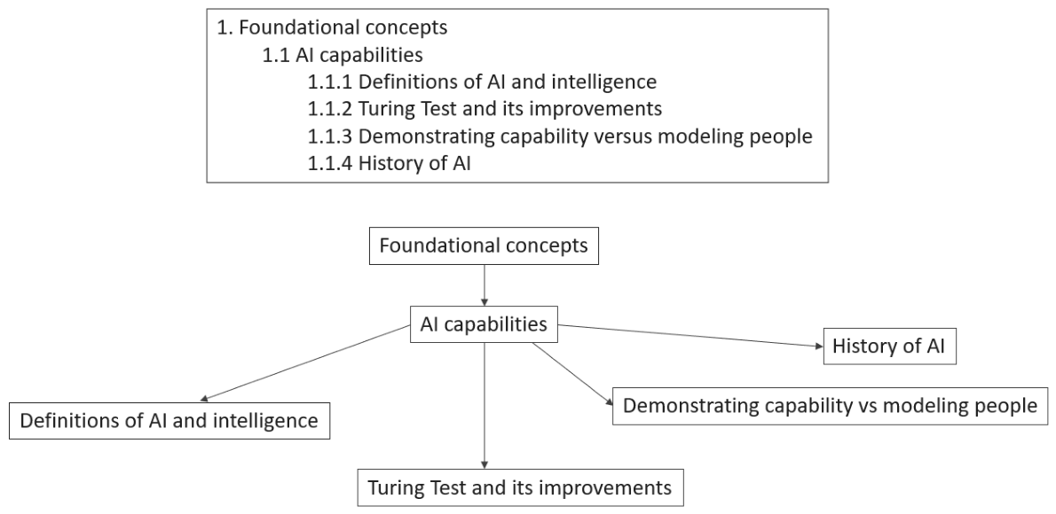
The knowledge graph used in this experiment is derived from a computer science taxonomy (Rowe, 2022). The knowledge graph is composed of 67 KNs derived from taxonomy headings. Prerequisite relationships exist between KNs that are higher in the taxonomy and those KNs that are immediately beneath them. This technique of determining prerequisites is called elaboration (Morrison et al., 2019). Figure 6 shows an example of using this AI taxonomy to derive a knowledge graph with prerequisite relationships.

3.2.2. Learner Profile

The learner profile is derived from questionnaire responses from 12 graduate students at an institution of higher learning (a large enough sample to examine the validity of algorithmic results). Expanding the questionnaire to a larger group of students is one opportunity for future work. The learners were asked to do the following:

• Report their perceived cognitive levels for each of the 67 KNs in the knowledge graph. Recall that cognitive levels can be 1, 2, 3, or 4, where 1 indicates a low understanding of the topic and 4 indicates an ability to read and understand technical LMs on the topic.
• Identify up to 5 goal KNs from the available 67.
• Report their degrees of preference for each content type on a scale of $\{1,2\dots ,9\}$, where 1 indicates most preferred and 9 indicates least preferred. The content types are research, website, discussion, educational, news article, do it yourself, PowerPoint, lecture, and textbook excerpt.
• Indicate their preferred media type with the choices: video, written, and none.
• Indicate their minimum and maximum preferred times for committing to complete a PLP in minutes.

Table 7. Subset of learner profile data for Section 4.

Student ID	Num. of Goal KNs	Avg. Cog. Level	Preferred Media	Min. Pref. Time (min)	Max. Pref. Time (min)
0	4	1.88	Text	360	1200
1	5	1.45	None	2400	4800
2	5	2.13	Video	30	90
3	18	1.42	Text	15	60
4	5	1.76	Video	20	90
5	5	1.72	Video	5	60
6	5	2.57	Video	10	30
7	15	2.22	Video	30	90
8	5	1.28	Video	30	90
9	5	1.64	Video	30	120
10	5	2.27	Video	30	120
11	5	2.93	Video	10	60

is a summary of some of the learner profile data. These data are included to assist the discussion in Section 4. Students 3 and 7 provided more than 5 KNs, which may complicate the satisfaction of the topic balance and time interval constraints.

3.2.3. Learning Materials

The LM metadata are available in the data package. These LMs were primarily collected by performing internet searches on the KNs. The LM metadata consist of the following fields.

• Difficulty Level: LMs are assigned difficulty $\in \{1,2,3,4\}$, where 1 is easy, 2 is medium, 3 is hard, and 4 is very hard. An example of 4 is a journal article on a given topic.
• Engagement Type: LMs can be text or video.
• Content Type: LMs can be one of the following content types: research, website, discussion, educational, news article, do it yourself, PowerPoint, lecture, or textbook excerpt.
• Duration: The estimated duration of the LM in minutes and seconds.
• CTML Compliance: LMs have the fields coherence principle, segmenting principle, worked example principle, signaling principle, spatial contiguity principle, temporal contiguity principle, modality principle, redundancy principle, personalization principle, voice principle, and sourcing principle.
• KNs Covered: This piece of metadata describes the KNs covered by each LM.
• Description: Each LM has an English text description. In the case of research articles, the abstract is used for this description.

3.2.4. Specifying the Design Values

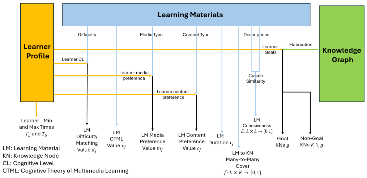
Based on the knowledge graph, learner profile, and LMs discussed in the previous section, this section describes the specification of design values for corresponding instances of the multi-objective LM selection and sequencing problems (the general problems are described in Section 3.1.1 and Section 3.1.5, respectively). Figure 7 shows which data from the learner profile, LMs, and knowledge graph are used to derive the various values. The LM selection design values are derived as follows.

• CTML Value ($v_j$): The LM rubric grades LMs according to their compliance with the following CTML principles: multimedia, coherence, segmenting, worked example, signaling, spatial contiguity, temporal contiguity, modality, redundancy, personalization, voice, and sourcing. If an LM is not multimedia (text-only, audio-only, etc.), then it receives a 1 in the multimedia category and it is not scored for the remaining CTML categories (as CTML principles only apply for multimedia LMs (Mayer & Fiorella, 2022)). In the data package, the score 0 is indicated when a particular CTML category does not apply to an LM, as is the case when LMs are not multimedia. In measuring CTML compliance, the multimedia score is the most important, as this is an estimate of how consistently multimedia messages are used in the LM. To calculate $v_j$ for LM ${\ell }_j$, we take the average of the non-zero CTML principle scores multiplied by the multimedia principle score divided by 4. An example is as follows: if the CTML average is $3.25$ and the multimedia principle score is 3, the CTML value score is $3.25·0.75=2.44$.
• LM Difficulty Matching Value ($d_j$): The difficulty matching value $d_j$ for the jth LM is calculated by taking the fraction of the KNs covered by LM ${\ell }_j$ for which the learner’s cognitive level for the KN matches the LM difficulty level. For instance, if LM ${\ell }_j$ covers two KNs, and the LM difficulty matches the learner’s cognitive level for only one of these KNs, then $d_j=0.5$.
• LM Media Preference Value $\left(m_j\right)$: The media preference value of the jth LM is 1 if the LM media type is the same as the learner’s preferred media type and 0 otherwise.
• LM Content Preference Value $\left(c_j\right)$: The content preference value $c_j$ of the jth LM is 1 if the LM content type is their most preferred type, $0.9$ if it is their second most preferred type, and so forth to the least preferred of the nine types, which is assigned $0.2$.
• LM Preference Value ($o_j$): The preference value of the jth LM is $o_j={\displaystyle \frac{m_j+c_j}{2}}$ in the case that the learner has a media preference; otherwise, $o_j=c_j$.
• LM Duration ($t_j$): The duration of the jth learning material is $t_j$.
• LM to LM Cohesiveness ($E:L\times L$): LM cohesiveness is measured for each pair of LMs through a three-step process. The first step uses the sentence-BERT model “all-mpnet-base-v2” to transform the LM text descriptions to a 768-dimensional vector (Reimers & Gurevych, 2019). The second calculates the cosine similarity between these embeddings. The final step normalizes the cosine similarity to the interval $[0,1]$.
• Goal KNs (g): Take the learner’s goal KNs and, consulting the knowledge graph, include all KNs that are prerequisites for these goals (the root KN is added as a goal for all learners).
• Non-Goal KNs ($K\setminus G$): All of the KNs in K that are not the learner’s goal KNs or prerequisites to it.

In the case of the LM selection problem, the coherence, segmenting, multiple-document integration, and topic balance values are calculated exclusively using the LM decision variables, the many-to-many function describing how the LMs cover the KNs, and the sets of goal and non-goal KNs. In the case of the LM sequencing problem, the design values are simpler to specify. The LM difficulty values are properties of the LMs, and the prerequisite and interleaving calculations are taken directly from the DAG and the many-to-many relationship between the LMs and the KNs. The learner profile is not consulted for the LM sequencing problem, as shown in Figure 3.

3.3. Algorithm Design

The following is a description of the algorithms used in solving the LM selection and sequencing problems, along with a description of the test of statistical significance used to validate their results.

3.3.1. LM Selection Algorithm Design

Evolutionary algorithms are a common approach to solving NP-hard PLP problems (Machado et al., 2021). Given the NP-completeness of the LM selection problem, the encoding of the LMs as $0/1$, and the competing objectives, a multi-objective genetic algorithm is a natural fit. Two possible choices for a multi-objective algorithm include the NSGA-II algorithm (Deb et al., 2002) and the Non-Dominated Sorting Genetic Algorithm III (NSGA-III) (Deb & Jain, 2014; Jain & Deb, 2014). The NSGA-II algorithm tends to perform better with three or less objectives, and the NSGA-III algorithm is better at maintaining population diversity when more than three objectives are considered. This work took the approach of combining subsets of the nine objectives to reduce the problem to three objectives, dividing them based on the average rubric score (the desired metric), the combined normalized LM compliance score, and the combined normalized KN compliance score. With three objectives, the NSGA-II algorithm becomes an acceptable approach. The NSGA-II (Deb et al., 2002) algorithm was used as implemented by the PyGAD Python library (Gad, 2023), with each chromosome consisting of the sequence of 365 LM decision variables. The multiple objectives enable the algorithm to identify a well-rounded set of PLPs for learners, such that the PLPs score well in most categories, rather than emphasizing PLPs that achieve excellent scores in a few categories and poor scores in others. Most of the effort in using this NSGA-II implementation was in designing the fitness function and the initial population function.

Initially, attempts were made to directly implement the PLP rubric categories as these objectives, but they were not sufficiently sensitive to small improvements, resulting in the NSGA-II quickly converging on poor solutions. Through experimentation, three combined objectives consistently yielded the strongest results, as indicated by the average rubric score. To create these three combined objectives, the nine objectives described in Section 3.1.1 were first normalized on the interval $[0,1]$ before using them to calculate the three fitness function objectives. The equations used to calculate the normalized objectives using their values from their decision problem description in Section 3.1.1 are as follows.

• Normalized CTML Value: $V_N={\displaystyle \frac{V_p-1}{3}}$
• Normalized Difficulty Matching Value: $D_N=D_p$
• Normalized Learner Preference Value: $O_N=O_p$
• Max Time Compliance:

  $$T_{max}=\left\{\begin{array}{cc}1,\hfill & \mathrm{if}{T}_p\le T_U\hfill \\ 1-{\displaystyle \frac{|T_U-T_p|}{0.2T_U}},\hfill & \mathrm{if}{T}_U<T_p<1.2T_U\hfill \\ 0,\hfill & \mathrm{if}{T}_p\ge 1.2T_U\hfill \end{array}\right.$$
• Min Time Compliance:

  $$T_{min}=\left\{\begin{array}{cc}1,\hfill & \mathrm{if}{T}_p\ge T_L\hfill \\ 1-{\displaystyle \frac{|T_L-T_p|}{0.2T_L}},\hfill & \mathrm{if}0.8T_L<T_p<T_L\hfill \\ 0,\hfill & \mathrm{if}{T}_L\le 0.8T_L\hfill \end{array}\right.$$
• Normalized Time Value: $T_N=\min (T_{min},T_{max})$. Without this step, $T_N$ would vary between $0.5$ and 1, as either $T_{max}$ or $T_{min}$ would always equal 1.
• Normalized Cohsiveness Value: $E_N=E_p$
• Normalized Coherence Value:

  $$C_N=\left\{\begin{array}{cc}0,\hfill & \mathrm{if}{C}_p>1\hfill \\ 1-C_p,\hfill & \mathrm{if}{C}_p\le 1\hfill \end{array}\right.$$
• Normalized Segmenting Value:

  $$S_N=\left\{\begin{array}{cc}1,\hfill & \mathrm{if}{S}_p=1\hfill \\ 1-{\displaystyle \frac{S_p-1}{3}},\hfill & \mathrm{if}1<S_p\le 4\hfill \\ 0,\hfill & \mathrm{if}{S}_p>4\hfill \end{array}\right.$$
• Normalized Multiple-Document Integration Principle Value:

  $$M_N=\left\{\begin{array}{cc}{\displaystyle \frac{M_p}{4}},\hfill & \mathrm{if}{M}_p<4\hfill \\ 1,\hfill & \mathrm{if}{M}_p\ge 4\hfill \end{array}\right.$$
• Normalized Balanced Cover:

  $$B_N=\left\{\begin{array}{cc}1-{\displaystyle \frac{B_p}{0.7}},\hfill & \mathrm{if}{B}_p<0.7\hfill \\ 0,\hfill & \mathrm{if}{B}_p\ge 0.7\hfill \end{array}\right.$$

The next step is to combine related normalized objectives and map them to the interval $[1,4]$ (chosen to be consistent with the average PLP rubric score). Consider the normalized values $D_N,V_N,O_N,E_N,B_N,M_N,C_N,S_N,T_N$ for a given candidate PLP p. Then, LM and KN compliance are defined as follows:

$$LM\_Compliance=3\left({\displaystyle \frac{V_N+D_N+O_N+T_N+E_N}{5}}\right)+1$$

$$KN\_Compliance=3\left({\displaystyle \frac{B_N+M_N+C_N+S_N}{4}}\right)+1$$

Of these two scores, $LM\_Compliance$ quantifies the average degree of fitness of the LMs for the learner but ignores the degree to which they satisfy their learning goals. In contrast, $KN\_Compliance$ gives information about how well the LMs meet the learner’s goals but ignores their degrees of fitness for the learner.

Finally, we have the objective $Rubric\_Average$, which is the average of the rubric scores of the candidate PLP according to Table 4. Ultimately, $Rubric\_Average$ is the score that should be maximized, but including $LM\_Compliance$ and $KN\_Compliance$ allows the genetic algorithm to continue to discover better solutions even in cases where marginal improvements to individual rubric categories are insufficient to impact the rubric score.

The fitness function is designed such that all candidate PLPs are feasible solutions and are scored accordingly. The exception to this rule is the case where $\left|p\right|<2$. The cohesiveness value $E_p$ is undefined when there are fewer than two LMs, so, in this case, the three fitness values are set to 1 (the lowest score).

In addition to the fitness function, an initial population function was implemented. In this function, a random choice is made from the LMs that cover the goal KNs until all goal KNs are covered and time constraints are met (goal KNs are deleted as LMs are identified that cover them). Once all goal KNs are covered, if $T_p<T_L$, the function randomly chooses from the remaining unselected LMs until $T_L\le T_p\le T_U$. Partial solutions are abandoned in the case that no LMs covering the remaining goal KNs are options such that $T_p\le T_U$ (where $T_p$ includes the time of the partial solution so far summed with the time of any of the remaining LMs). In the case that the algorithm makes 10,000 unsuccessful consecutive attempts to generate a chromosome, the remaining population is generated by ignoring the time constraints and simply randomly selecting LMs until all goal KNs are covered.

Following the design of the fitness and initial population functions, the next step was to choose parameters for the NSGA-II algorithm. The single-point crossover option was chosen as it is likely to preserve the structure of high-value parents in their offspring (Coello et al., 2007). We used the swap mutation option to minimally impact a given candidate solution (but still allow for exploring different possible combinations of LMs). The NSGA-II literature recommends setting the mutation probability to $1/n$, where n is the number of decision variables ($n=365$ in this case), and to sweep the crossover probability between $0.8$ and $0.95$ in $0.01$ increments (Deb et al., 2002; Ramesh et al., 2012). After performing this parameter sweep, the crossover probability of $0.9$ returned the highest average rubric score across the student population. Additional parameters recommended in the NSGA-II literature include a population size of 100 and 500 generations (Ramesh et al., 2012). As a result, the following configuration was used in the NSGA-II implementation:

• Solutions per population: 100;
• Number of generations: 500;
• Crossover type: single-point crossover;
• Mutation type: swap;
• Crossover probability: $0.84$;
• Mutation probability: $1/365$.

Finally, the NSGA-II algorithm was run 30 times across the 12 students to observe the means and variances of the rubric scores of the returned PLPs. The returned solutions from these 30 iterations were moved forward to the LM sequencing problem.

3.3.2. LM Sequencing Algorithm Design

When designing the algorithm to solve the multi-objective LM sequencing problem, the first step is to design the fitness function. This fitness function includes the values of $H_p$ (difficulty sequencing), $R_p$ (prerequisite sequencing), and $I_p$ (interleaving). For each value, the maximum number of violations is calculated assuming that every penalty occurs. These are denoted as $H_M$, $R_M$, and $I_M$. Next, we divide the values for candidate solution p by these maximum values. This normalizes the individual objectives within $[0,1]$, with the goal being to minimize these objectives. They are then combined into a single fitness function $fitness=(H_p/H_M+R_p/R_M+I_P/I_M)/3$ with equal weighting for each objective.

As proven in Section 3.1.5, the LM sequencing problem is NP-complete, so a stochastic approach may be appropriate. To solve the sequencing problem, both the Random Hill Climber (RHC) algorithm and the simulated annealing (SA) algorithm start with a random sequence of the LMs. The RHC algorithm then randomly selects two indices in this random sequence and attempts to swap the positions of the two LMs with these indices, keeping the solution if it has a lower (better) $fitness$ value (each attempt uses two random indices in the sequence) (Russell & Norvig, 2021). The SA algorithm works similarly to the RHC but with a decreasing (cooling) probability of accepting an inferior solution (Russell & Norvig, 2021). In both cases, every time a better solution is found, the algorithm checks for the condition that the rubric score in each category is 4 (a perfect rubric score). If such a solution is found, the loop is broken and the solution returned.

Ten thousand iterations each were run for the RHC algorithm and the SA algorithm (each iteration included a fitness evaluation of the resultant solution). For the latter, a temperature schedule was selected for which the probability of accepting a step to a slightly worse solution began at $0.90$ and ended near 0. Specifically, “slightly worse” was taken to mean $0.1$ higher, which is $10\%$ of the range of the fitness function. As such, we selected an initial temperature of $T_1=0.95$ and a final temperature of $T_f=0.01$ (since $e^{-0.1/0.95}\approx 0.90$ and $e^{-0.1/0.01}\approx 4\times {10}^{-5}$). To calculate the cooling rate $\alpha$, we used the formula recommended by Kirkpatrick et al. (1983): $\alpha ={(T_m/T_1)}^{1/(m-1)}$, where $m=\mathrm{10,000}$, $T_1=0.95$, $T_m=0.01$, and therefore $\alpha =0.9995467$. The end result is that, as the SA algorithm comes close to 10,000 iterations, it will behave similarly to the RHC algorithm (only accepting better solutions).

For each student and for each of the 30 independent executions of the LM selection algorithm for each student (Section 3.3.1), we used the resulting LM set as input to the LM sequencing algorithms. We performed 30 independent executions each of the RHC algorithm and the SA algorithm against each LM set, for a total of 900 executions of each sequencing algorithm per student. These data were then used to determine the average mean and average variance for the three sequencing rubric categories and the average rubric score for each student.

3.3.3. Algorithm Variance Statistical Test

Given that the LM selection and sequencing algorithms are stochastic in nature, their returned solutions may be random and therefore not personalized to the student profiles. To test this possibility, the variances of the 30 iterations for the LM selection problem are compared to what would be expected from a discrete uniform random distribution. This distribution would result from randomly choosing among $\{1,2,3,4\}$ for each PLP rubric category for a sufficient number of iterations. For each student profile, the average of one of the nine PLP rubric score variances would be $(4^2-1)/12=1.25$ if taken from a discrete uniform random distribution, and the average of nine such variances would be $1.25/9=0.139$, whereas the average of three such variances would be $1.25/3=0.417$ in the case of the LM sequencing problem.

The expected variance of the LM selection and sequencing problems can then be used to calculate the critical point of statistical significance to determine whether the 30 iterations of the algorithms are likely to come from the discrete uniform distribution. The one-sided variance test is accomplished using the ${\chi }^2$ test of single variance (Sellers, 2023) along with $p=0.05$. The alternative hypothesis for each student profile is that the returned rubric average scores do not come from the discrete uniform random distribution, and the null hypothesis is that they do come from the discrete uniform random distribution.

The goal of this statistical test is to show that the variances of the rubric average scores of 30 algorithm samples for each student profile are less than the critical point $s^2$, the maximum threshold, so that, if the measured variance is greater than $s^2$, the null hypothesis holds, and, if the measured variance is less than $s^2$, the alternative hypothesis holds. This experiment is left-tailed, because the alternative hypothesis requires that the measured variance is less than the critical point.

Given that 30 samples implies 29 degrees of freedom ($30-1$ samples), a lookup table yields ${\chi }^2=17.708$. The formula to calculate the critical value is ${\chi }^2=(n-1)s^2/{\sigma }^2$, where $s^2$ is the measured variance of the samples, ${\sigma }^2$ is the predicted variance of the population, and n is the number of samples. Solving for $s^2$ and using the previously discussed numbers yields $s^2={\chi }^2{\sigma }^2/(n-1)=(17.708·0.139)/29=0.0849$ in the case of LM selection and $s^2=(17.708·0.417)/29=0.254$ in the case of LM sequencing.

Therefore, given 30 samples of the NSGA-II algorithm for a student profile, if the measured variance of the selection rubric average is less than $0.8049$, the alternative hypothesis is accepted (otherwise, the null hypothesis is accepted). Likewise, given 30 samples of the RHC or SA algorithms for a student profile, if the measured variance of the sequence rubric average is less than $0.254$, the alternative hypothesis is accepted.

4. Results

This section reviews the results of the multi-objective LM selection and sequencing problem experiments discussed in Section 3. The lowest combined rubric average score was $3.19$ for Student 11, and the highest combined rubric average score was 3.54 for Student 9. In all cases, the NSGA-II, RHC, and SA algorithms passed the ${\chi }^2$ tests of the hypotheses. In the case of the NSGA-II algorithm, a tension is observed between the topic balance and time interval objectives in cases where students had relatively low time restrictions and a relatively large number of goals. This tension led to high variances in these objectives as the NSGA-II algorithm either sought to optimize the topic balance objective at the expense of the time interval objective or vice versa. Furthermore, a relatively large number of unique decision variable assignments was observed, which resulted in weaker scores in the Pareto front, in comparison to a relatively small number that resulted in the stronger scores.

4.1. LM Selection Results

Table 8. Mean rubric scores averaged across 30 independent NSGA-II-based LM selection experiments and 900 RHC-based LM sequencing experiments.

	LM Selection—NSGA-II									LM Sequencing—RHC
Student ID	CTML	Difficulty Matching	Learner Preference	Time Interval	Cohesiveness	Coherence	Segmenting	Multiple-Doc. Int.	Topic Balance	Difficulty Seq.	Prerequisite Seq.	Interleaving	Overall Average
0	3.03	2.43	3.63	4.00	3.00	3.90	4.00	1.00	3.90	4.00	4.00	4.00	3.41
1	3.00	2.27	3.00	3.97	3.00	2.13	4.00	3.67	3.17	4.00	4.00	4.00	3.35
2	3.80	3.00	3.40	3.93	3.00	3.83	4.00	1.00	1.63	4.00	4.00	4.00	3.30
3	3.07	3.90	2.97	1.00	3.00	4.00	4.00	1.00	3.93	4.00	4.00	4.00	3.24
4	3.93	3.83	3.93	3.97	3.00	3.10	4.00	1.00	3.50	4.00	4.00	4.00	3.52
5	3.37	2.47	3.37	4.00	3.10	3.37	4.00	1.00	2.90	4.00	4.00	4.00	3.30
6	4.00	2.90	3.00	1.00	3.00	4.00	4.00	1.00	4.00	4.00	4.00	4.00	3.24
7	3.53	3.10	3.20	1.83	3.00	4.00	4.00	1.00	2.87	4.00	4.00	4.00	3.21
8	3.03	3.00	3.03	4.00	3.00	3.60	4.00	1.00	3.33	3.98	3.82	4.00	3.32
9	3.97	2.90	4.00	4.00	3.43	4.00	4.00	1.00	3.73	3.94	3.50	4.00	3.54
10	3.77	3.37	3.43	4.00	3.00	4.00	4.00	1.00	3.90	3.97	3.84	4.00	3.52
11	3.63	2.37	3.00	3.00	3.00	3.90	4.00	1.00	2.37	4.00	4.00	4.00	3.19

shows the average PLP rubric scores obtained by the NSGA-II-based LM selection algorithm for each student along with the average overall scores; whereas

Table 9. Variances of PLP rubric scores across 30 independent executions.

Student ID	CTML	Difficulty Matching	Learner Pref. Match.	Time Interval	Cohesiveness	Coherence	Segmenting	Multiple-Doc. Int.	Topic Balance	Rubric Average
0	0.0333	0.2540	0.2402	0.0000	0.0000	0.0931	0.0000	0.0000	0.0931	0.0020
1	0.0000	0.2023	0.0000	0.0333	0.0000	0.1195	0.0000	0.2299	0.1437	0.0020
2	0.1655	0.2759	0.2483	0.0644	0.0000	0.1437	0.0000	0.0000	0.6540	0.0048
3	0.0644	0.0931	0.0333	0.0000	0.0000	0.0000	0.0000	0.0000	0.0644	0.0015
4	0.0644	0.1437	0.0644	0.0333	0.0000	0.0931	0.0000	0.0000	0.2586	0.0025
5	0.2402	0.4644	0.2402	0.0000	0.0931	0.2402	0.0000	0.0000	2.1621	0.0082
6	0.0000	0.0931	0.0000	0.0000	0.0000	0.0000	0.0000	0.0000	0.0000	0.0011
7	0.2575	0.1621	0.1655	1.4540	0.0000	0.0000	0.0000	0.0000	1.5678	0.0125
8	0.0333	0.0000	0.0333	0.0000	0.0000	0.2483	0.0000	0.0000	0.2989	0.0000
9	0.0333	0.0931	0.0000	0.0000	0.2540	0.0000	0.0000	0.0000	0.3402	0.0055
10	0.1851	0.3092	0.2540	0.0000	0.0000	0.0000	0.0000	0.0000	0.1621	0.0032
11	0.3092	0.3782	0.0000	1.8621	0.0000	0.0931	0.0000	0.0000	0.9989	0.0119

shows the variances of the PLP rubric scores along with the averages of the individual rubric score variances. For each student profile, the average of the PLP rubric score variances is substantially below $((4^2-1)/12)/9=0.139$, which would be the expected value if each individual rubric score were drawn from a discrete uniform random distribution over $\{1,2,3,4\}$. This suggests that the NSGA-II fitness functions are consistent with the underlying PLP rubric scores. The remainder of this section more closely examines the results for Students 5, 7, and 11, which have the largest average rubric score variances, and Student 1, which is an interesting example of the tradeoffs evident in the LM selection problem.

For Students 7 and 11, the variances of the time interval and topic balance scores exceed $0.9989$ (in fact, three of them exceed $1.25$). These effects are directly attributable to features of the students’ learner profiles. Specifically, Student 7 specified 15 goal KNs, which the selection algorithm apparently struggled to cover without exceeding a maximum preferred time of $T_U=90$ min (a concrete example of the tension between these two objectives). Similarly, Student 11 specified $T_U=60$ and five goal KNs. It is likely that both of these students would have obtained better-scoring PLPs had they either reduced the number of goal KNs or increased the upper time limit.

Table 10. Range of optimal PLP scores for Student 7.

CTML	Diff. Match	Learner Pref.	Time Int.	Cohesiveness	Coherence	Segmenting	Mult.-Doc. Int.	Topic Balance	Rubric Avg.
3	2	3	1	3	4	4	1	4	2.78
4	3	3	1	3	4	4	1	3	2.89
3	3	3	2	3	4	4	1	3	2.89
3	3	3	1	3	4	4	1	4	2.89
4	3	3	2	3	4	4	1	2	2.89
4	4	3	2	3	4	4	1	1	2.89
4	3	3	4	3	4	4	1	1	3.00
3	3	3	2	3	4	4	1	4	3.00
4	3	4	4	3	4	4	1	1	3.11
4	4	4	3	3	4	4	1	1	3.11
4	4	4	4	3	4	4	1	1	3.22

shows the scores of the LM selection solutions that were the best-scoring solutions according to the PLP rubric in at least 1 of the 30 independent executions for Student 7. The topic balance and time interval scores are negatively correlated, again resulting in the algorithm exploring a Pareto front and producing large variances for these scores, as shown in Table 9. The best-scoring solution had CTML, difficulty, and learner preference scores of 4, implying that this solution yielded a subset of LMs that matched the learner in these categories and fit within Student 7’s time constraints.

Table 11. Range of optimal PLP scores for Student 11.

CTML	Diff. Match	Learner Pref.	Time Int.	Cohesiveness	Coherence	Segmenting	Mult.-Doc. Int.	Topic Balance	Rubric Avg.
3	2	3	1	3	3	4	1	4	2.67
4	2	3	1	3	4	4	1	3	2.78
3	3	3	1	3	3	4	1	4	2.78
3	3	3	1	3	4	4	1	3	2.78
4	3	3	1	3	4	4	1	2	2.78
3	2	3	4	3	4	4	1	2	2.89
2	2	3	4	3	4	4	1	3	2.89
4	3	3	1	3	4	4	1	3	2.89
4	2	3	4	3	4	4	1	1	2.89
4	2	3	4	3	4	4	1	2	3.00
4	2	3	3	3	4	4	1	3	3.00
4	3	3	4	3	4	4	1	1	3.00
4	1	3	4	3	4	4	1	3	3.00
3	2	3	4	3	4	4	1	3	3.00
3	4	3	4	3	4	4	1	1	3.00

shows the scores of the LM selection solutions that were the best-scoring solutions according to the PLP rubric in at least 1 of the 30 independent executions for Student 11. As with Student 7, topic balance and time interval are negatively correlated, which is indicated by their large variances in Table 9.

Interestingly, Student 5 also specified $T_U=60$ and five goal KNs. In this case, while the LM selection algorithm consistently found PLPs that satisfied the time constraint, it struggled in other areas. Consider the comparatively high variances of the scores for topic balance, CTML matching, difficulty matching, and learner preference matching.

Table 12. Range of optimal PLP scores for Student 5.

CTML	Diff. Match	Learner Pref.	Time Int.	Cohesiveness	Coherence	Segmenting	Mult.-Doc. Int.	Topic Balance	Rubric Avg.
3	2	3	4	3	3	4	1	4	3.00
4	3	4	4	3	4	4	1	1	3.11
4	3	4	4	4	4	4	1	1	3.22
4	4	4	4	3	4	4	1	1	3.22

provides additional insight into the sources of these variance scores. Specifically, the topic balance score is inversely correlated with each of the LM matching scores (CTML, difficulty, and learner preference). In other words, over multiple executions, the selection algorithm explores a Pareto front representing a tradeoff between topic balance and matching, resulting in the observed high variances.

Table 13. Range of optimal PLP scores for Student 1.

CTML	Diff. Match	Learner Pref.	Time Int.	Cohesiveness	Coherence	Segmenting	Mult.-Doc. Int.	Topic Balance	Rubric Avg.
3	2	3	4	3	2	4	3	4	3.11
3	3	3	4	3	2	4	3	3	3.11
3	2	3	4	3	2	4	4	3	3.11
3	2	3	3	3	3	4	4	3	3.11
3	2	3	4	3	3	4	4	3	3.22
3	3	3	4	3	2	4	3	4	3.22
3	3	3	4	3	2	4	4	3	3.22
3	3	3	4	3	3	4	3	3	3.22

shows the top-scoring solutions across 30 iterations for Student 1. None of the solutions have coherence scores of 4, and most have scores of 2 in this category, implying that the NSGA-II algorithm had difficulty finding subsets of LMs that both satisfied the student’s time constraints and covered their goal KNs (as there might not have been enough LMs covering their goal KNs to meet $T_L$). Moreover, multiple-document integration and topic balance are negatively correlated and never simultaneously reach 4, implying a potential lack of balance in the LM coverage of Student 1’s subset of goal KNs.

4.2. LM Sequencing Results

For each of the 12 student profiles, each of the 900 executions of the SA-based LM sequencing algorithm (30 executions each on 30 sets of LMs) yielded a rubric average score, as well as for the RHC-based algorithm. The means and variances of these scores are shown for each student in

Table 14. Average mean and variance for 30 iterations of the SA algorithm.

	Difficulty		Prerequisite		Interleaving		Rubric Avg.
ID	Mean	Var	Mean	Var	Mean	Var	Mean	Var
0	4.00	0.00	4.00	0.00	4.00	0.00	4.00	0.00
1	3.01	0.01	3.42	0.24	4.00	0.00	3.48	0.03
2	4.00	0.00	4.00	0.00	4.00	0.00	4.00	0.00
3	3.99	0.01	4.00	0.00	4.00	0.00	4.00	0.00
4	4.00	0.00	4.00	0.00	4.00	0.00	4.00	0.00
5	4.00	0.00	4.00	0.00	4.00	0.00	4.00	0.00
6	4.00	0.00	4.00	0.00	4.00	0.00	4.00	0.00
7	3.99	0.01	3.99	0.01	4.00	0.00	3.99	0.00
8	3.97	0.03	3.93	0.07	4.00	0.00	3.97	0.01
9	3.93	0.07	3.61	0.24	4.00	0.00	3.84	0.03
10	3.99	0.01	3.84	0.13	4.00	0.00	3.94	0.02
11	4.00	0.00	4.00	0.00	4.00	0.00	4.00	0.00

(simulated annealing) and

Table 15. Average mean and variance for 30 iterations of the RHC algorithm.

	Difficulty		Prerequisite		Interleaving		Rubric Avg.
ID	Mean	Var	Mean	Var	Mean	Var	Mean	Var
0	4.00	0.00	4.00	0.00	4.00	0.00	4.00	0.00
1	4.00	0.00	4.00	0.00	4.00	0.00	4.00	0.00
2	4.00	0.00	4.00	0.00	4.00	0.00	4.00	0.00
3	4.00	0.00	4.00	0.00	4.00	0.00	4.00	0.00
4	4.00	0.00	4.00	0.00	4.00	0.00	4.00	0.00
5	4.00	0.00	4.00	0.00	4.00	0.00	4.00	0.00
6	4.00	0.00	4.00	0.00	4.00	0.00	4.00	0.00
7	4.00	0.00	4.00	0.00	4.00	0.00	4.00	0.00
8	3.98	0.02	3.82	0.15	4.00	0.00	3.93	0.02
9	3.94	0.06	3.50	0.25	4.00	0.00	3.81	0.03
10	3.97	0.03	3.84	0.13	4.00	0.00	3.94	0.02
11	4.00	0.00	4.00	0.00	4.00	0.00	4.00	0.00

(Random Hill Climbing). Overall, both algorithms returned acceptable results for the PLP rubric. However, for the Student 1 learner profile, the best LM sequences obtained by the SA-based algorithm had average difficulty and prerequisite scores of $3.02$ and $3.44$, respectively. The LM sets for Student 1 average approximately 80 elements, compared to roughly 17 for Student 7. This suggests that the SA algorithm’s probabilistic acceptance of inferior neighboring solutions is a disadvantage in the case of larger LM solution sets. In contrast, Students $0,2,4,5,6,8,9,10,\mathrm{and}11$ all had LM sets averaging fewer than 10 elements, and, in some cases, the SA algorithm was able to outperform the RHC algorithm in these smaller solution sets. This suggests that the ability to escape locally optimal solutions may be a valuable algorithmic feature in some instances.

As a general takeaway regarding the RHC algorithm, the variances of the difficulty, prerequisite, and interleaving scores are low across the 12 students, and the mean scores are high (close to $4.0$). In the case of interleaving, the algorithm matched all students with solutions that scored $4.0$. This suggests that, despite interleaving and prerequisite sequencing being sufficient conditions for NP-completeness in the general case of the sequencing problem, the real-world data in this research do not translate into difficult problem instances.

The inclusion of the segmenting and topic balance objectives in the LM selection problem may be the reason that the LMs sequencing problem instances are easier than expected. In the case of the segmenting objective, the NSGA-II algorithm tries to select LMs that cover less than two KNs on average (recall that the many-to-many characteristic of LM sequencing problems was necessary for both proofs of NP-completeness). Some cases of the LM sequencing problem actually reduce to many-to-one, which has objectives that are PTIME in isolation (see Table 6). In the case of the topic balance objective, the NSGA-II algorithm tries to select LMs that cover the goal KNs evenly. Recall that the algorithm proving that the many-to-one LM sequencing problem was PTIME in the case of the interleaving objective relied on a distribution of LMs across at least two KNs to avoid violations of the interleaving objective in the final stretch. Reasonably, a topic balance score of 3 or 4 might imply an easier problem instance in satisfying the interleaving objective, even with larger solution sets (such as was the case with Student 1, who averaged close to 80 LMs in a solution). In the cases of Students 7 and 11, who displayed tension between topic balance and time interval, this was due to tight time constraints, and their LM selection solutions either violated their time constraints, with an even distribution across goal KNs, or satisfied their time constraints, resulting in a smaller search space in the LM sequencing problem. In conclusion, in the case of the twelve student profiles, the LM selection problem in combination with the NSGA-II algorithm generates relatively “easy” LM sequencing problem instances despite the NP-completeness of the general sequencing problem.

5. Discussion

One of the main implications of this study is that CTML and similar educational theory best practices can be meaningfully transformed into problems and their associated design variables, enabling them to be processed by AI algorithms to produce PLPs. Historically, PLP research has not formed a connection between CTML and PLP design, instead focusing on learning styles to assist in matching LMs with students (A. Li et al., 2026; H. Li et al., 2023; Machado et al., 2021; Nabizadeh et al., 2020; Son et al., 2021; Wang & Fu, 2021) or on Bloom’s Taxonomy as a means of quantifying a student’s cognitive levels to facilitate matching with LMs of appropriate difficulty (A. Li et al., 2026; Mochocki et al., 2025). The ability to rank LMs and PLPs according to their compliance with CTML principles has the potential to impact e-learning by providing students with sequences of LMs that are more likely to assist them in managing their cognitive loads as they move towards their specific learning goals (Mayer & Fiorella, 2022; Mutlu-Bayraktar et al., 2019). Despite this important contribution, the rubrics may not adequately rank LMs and PLPs according to CTML (possibly through human error in rubric design or in rating the body of LMs used in this experimental design) and thus warrant additional testing and refinement.

The approach to the sequencing PLP problem outlined in this paper assumes that PLPs that maximize elaboration, difficulty, and interleaving (Carey, 2015) would have superior student outcomes in comparison to approaches that only maximize one. Additionally, the discussion of many-to-many vs. many-to-one PLP problems in this paper primarily focuses on their respective impacts on the complexity of the LM sequencing problem. Beyond algorithmic complexity, these relationships are also likely to impact student learning outcomes for several reasons. First of all, the segmenting principle from CTML states that students learn better when LMs are presented in user-paced small segments rather than a continuous stream of information (Mayer, 2024; Mayer & Fiorella, 2022). We postulate that the segmenting principle implies that many-to-one PLP problems will facilitate enhanced learning as students receive these “chunked” LM segments (as such LMs in a many-to-one construction will be more targeted than in a many-to-many construction). The possible superiority of the many-to-one PLP problem is strengthened by the observation that many-to-one PLP problems will always have a perfect score of 4 in the segmenting category of the PLP rubric, because all LMs included in every possible candidate PLP will only cover one KN (the definition of many-to-one) (Mochocki et al., 2024). Additionally, students might have varying cognitive levels for multiple KNs covered by a single LM in a many-to-many environment (A. Li et al., 2026), which makes the problem of selecting LMs that match their cognitive levels across all goal KNs more challenging. In contrast, in a many-to-one PLP problem, an algorithm can more easily provide students with LMs that reflect their measured cognitive levels for each goal KN (Mochocki et al., 2025). While these theories of PLP best practices to improve student learning outcomes seem reasonable based on the reviewed literature, they warrant further validation via human testing.

Additional limitations include the relatively small sample size of LMs and the choice of the NSGA-II algorithm. Future studies should include more than 365 LMs to validate how the algorithm performs in a much larger search space. In general, having more LMs in the search space (assuming sufficient variety in metadata characteristics) implies that PLPs may exist that are more personalized to students and therefore are higher-scoring according to the rubric. Additionally, researchers should experiment with not combining the objectives in the LM selection problem and using other algorithms, such as the NSGA-III, that are designed to handle a greater number of objectives (Deb & Jain, 2014; Jain & Deb, 2014).

6. Conclusions

This paper addresses the problem of creating a personalized learning path, which is a sequence of LMs selected and sequenced on-demand for a learner using metadata derived from a knowledge graph, a learner profile, and a corpus of LMs. The novelty of this approach is the use of CTML, an empirically validated learning science, to derive a PLP rubric, which was then used to inform the entirety of the remaining PLP design process. This paper defines the LM selection and sequencing problems, describing objectives and constraints derived from this PLP rubric. The selection and sequencing problems are accompanied by proofs of computational complexity and a discussion of the implications of these proofs for various problem variations.

After the design of these problems, the paper demonstrates how real-world data can be reduced to problem instances that can be solved by metaheuristics and then graded according to the PLP rubric. The metaheuristics chosen for this task were the NSGA-II to select the subset of LMs and a Hill Climber and simulated annealing algorithm to sequence them. Finally, the algorithms were used to solve problem instances for 11 students to show that they could achieve adequate scores according to the rubric. The algorithms were also validated via a test of statistical significance, demonstrating that they did not produce results that came from the uniform randomized distribution across 30 iterations, providing evidence that the PLPs were personalized to the students. The final step of the PLP design process (validating the PLP rubric with human testing) is left for future work. The authors theorize that using an empirically tested learning science to inform the PLP design process will result in superior learning outcomes in students. As the rubrics, data, and code are publicly available, other researchers may use them to assist in attempts to validate or refute this central hypothesis by performing their own experiments.

References

1. Abu-Rasheed, H., Weber, C., Dornhöfer, M., & Fathi, M. (2023). Pedagogically-informed implementation of reinforcement learning on knowledge graphs for context-aware learning recommendations. In European conference on technology enhanced learning (Vol. 14200 LNCS, pp. 518–523). Springer. [Google Scholar] [CrossRef] [Scilit]
2. Acampora, G., Gaeta, M., & Loia, V. (2011). Hierarchical optimization of personalized experiences for e-Learning systems through evolutionary models. Neural Computing and Applications, 20, 641–657. [Google Scholar]
3. Altinpulluk, H., Kilinc, H., Firat, M., & Yumurtaci, O. (2020). The influence of segmented and complete educational videos on the cognitive load, satisfaction, engagement, and academic achievement levels of learners. Journal of Computers in Education, 7(2), 155–182. [Google Scholar] [CrossRef] [Scilit]
4. Benmesbah, O., Lamia, M., & Hafidi, M. (2021). A novel genetic algorithm for curriculum sequence optimization. Intelligent Decision Technologies, 15(3), 469–485. [Google Scholar] [CrossRef] [Scilit]
5. Benmesbah, O., Lamia, M., & Hafidi, M. (2023). An improved constrained learning path adaptation problem based on genetic algorithm. Interactive Learning Environments, 31(6), 3595–3612. [Google Scholar]
6. Bian, C., Dong, S., Li, C., Shi, Z., & Lu, W. (2017). Generation of adaptive learning path based on concept map and immune algorithm. In 2017 12th international conference on computer science and education (ICCSE) (pp. 409–414). IEEE. [Google Scholar]
7. Bian, C.-L., Wang, D.-L., Liu, S.-Y., Lu, W.-G., & Dong, J.-Y. (2019). Adaptive learning path recommendation based on graph theory and an improved immune algorithm. KSII Transactions on Internet and Information Systems (TIIS), 13(5), 2277–2298. [Google Scholar] [CrossRef] [Scilit]
8. Carey, B. (2015). How we learn: The surprising truth about when, where, and why it happens. Random House Trade Paperbacks. [Google Scholar]
9. Chang, T.-Y., & Ke, Y.-R. (2013). A personalized e-course composition based on a genetic algorithm with forcing legality in an adaptive learning system. Journal of Network and Computer Applications, 36(1), 533–542. [Google Scholar] [CrossRef] [Scilit]
10. Coello, C. A. C., Lamont, G. B., & Veldhuizen, D. A. V. (2007). Evolutionary algorithms for solving multi-objective problems. Springer. [Google Scholar]
11. Coursera Investor Relations. (2025). 2024 corporate impact report: Scaling global reach and technical skill development (Annual Impact Report). Coursera. Available online: https://s27.q4cdn.com/928340662/files/doc_downloads/2025/03/2024-Impact-Report_Coursera.pdf (accessed on 25 May 2026).
12. Deb, K., & Jain, H. (2014). An evolutionary many-objective optimization algorithm using reference-point-based nondominated sorting approach, part I: Solving problems with box constraints. IEEE Transactions on Evolutionary Computation, 18(4), 577–601. [Google Scholar] [CrossRef] [Scilit]
13. Deb, K., Pratap, A., Agarwal, S., & Meyarivan, T. (2002). A fast and elitist multiobjective genetic algorithm: NSGA-II. IEEE Transactions on Evolutionary Computation, 6(2), 182–197. [Google Scholar] [CrossRef] [Scilit]
14. Department of the Air Force. (2024). Digital university (du) platform assessment and privacy impact record (Official Institutional Report). Air Force Privacy Act Office. Available online: https://www.privacy.af.mil/Portals/26/Digital%20University%20(DU).pdf (accessed on 25 May 2026).
15. Fung, S., Tam, V., & Lam, E. Y. (2011). Enhancing learning paths with concept clustering and rule-based optimization. In 2011 IEEE 11th international conference on advanced learning technologies (pp. 249–253). IEEE. [Google Scholar] [CrossRef] [Scilit]
16. Gad, A. F. (2023). Pygad: An intuitive genetic algorithm python library. Multimedia Tools and Applications, 83, 58029–58042. [Google Scholar] [CrossRef] [Scilit]
17. Genevieve, C., Hamilton, L., & Chatterjee, A. (2024). 2024 online learning statistics. Available online: https://www.forbes.com/advisor/education/online-colleges/online-learning-stats/ (accessed on 20 February 2025).
18. Gomez-Gonzalez, M., & Jurado, F. (2012). Personalized e-learning using shuffled frog-leaping algorithm. In Proceedings of the 2012 IEEE global engineering education conference (EDUCON) (pp. 1–7). IEEE. [Google Scholar]
19. Hattie, J., & O’Leary, T. (2025). Learning styles, preferences, or strategies? An explanation for the resurgence of styles across many meta-analyses. Educational Psychology Review, 37(2), 31. [Google Scholar] [CrossRef] [Scilit]
20. Hnida, M., Idrissi, M. K., & Bennani, S. (2018). Automatic composition of instructional units in virtual learning environments. International Journal of Emerging Technologies in Learning, 13(6), 86–100. [Google Scholar] [CrossRef] [Scilit]
21. Jain, H., & Deb, K. (2014). An evolutionary many-objective optimization algorithm using reference-point-based nondominated sorting approach, part II: Handling constraints and extending to an adaptive approach. IEEE Transactions on Evolutionary Computation, 18(4), 602–622. [Google Scholar] [CrossRef] [Scilit]
22. Karp, R. M. (1972). Reducibility among combinatorial problems. In R. E. Miller, J. W. Thatcher, & J. Bohlinger (Eds.), Complexity of computer computations (pp. 85–103). Plenum. [Google Scholar] [CrossRef] [Scilit]
23. Khan Academy. (2025). Khan academy annual impact report: School year 2024–2025 (Annual Impact Report). Khan Academy. Available online: https://annualreport.khanacademy.org/ (accessed on 25 May 2026).
24. Kirkpatrick, S., Gelatt, C. D., Jr., & Vecchi, M. P. (1983). Optimization by simulated annealing. Science, 220(4598), 671–680. [Google Scholar] [CrossRef] [Scilit] [PubMed]
25. Kirschner, P. A. (2017). Stop propagating the learning styles myth. Computers & Education, 106, 166–171. [Google Scholar] [CrossRef] [Scilit]
26. Kozierkiewicz-Hetmańska, A., & Nguyen, N. (2011). A method for learning scenario determination and modification in intelligent tutoring systems. International Journal of Applied Mathematics and Computer Science, 21(1), 69–82. [Google Scholar] [CrossRef] [Scilit]
27. Li, A., Li, Y., & Gao, X. (2026). Personalized learning path recommendation based on knowledge graphs: A survey. Electronics, 15, 238. [Google Scholar] [CrossRef] [Scilit]
28. Li, H., Gong, R., Zhong, Z., Xing, L., Li, X., & Li, H. (2023). Research on personalized learning path planning model based on knowledge network. Neural Computing and Applications, 35(12), 8809–8821. [Google Scholar] [CrossRef] [Scilit]
29. Machado, M. d. O. C., Bravo, N. F. S., Martins, A. F., Bernardino, H. S., Barrere, E., & Souza, J. F. d. (2021). Metaheuristic-based adaptive curriculum sequencing approaches: A systematic review and mapping of the literature. Artificial Intelligence Review, 54(1), 711–754. [Google Scholar]
30. Martins, A. F., Machado, M., Bernardino, H. S., & de Souza, J. F. (2021). A comparative analysis of metaheuristics applied to adaptive curriculum sequencing. Soft Computing, 25(16), 11019–11034. [Google Scholar] [CrossRef] [Scilit] [PubMed]
31. Mayer, R. E. (2024). The past, present, and future of the cognitive theory of multimedia learning. Educational Psychology Review, 36(1), 8. [Google Scholar] [CrossRef] [Scilit]
32. Mayer, R. E., & Fiorella, L. (Eds.). (2022). The cambridge handbook of multimedia learning (3rd ed.). Cambridge University Press. [Google Scholar]
33. Mochocki, S. A., & Reith, M. G. (2025). Data package supporting research on personalized learning path problem derived from the cognitive theory of multimedia learning. Available online: https://scholar.afit.edu/facpub/2151 (accessed on 5 April 2025).
34. Mochocki, S. A., Reith, M. G., Borghetti, B. J., Peterson, G. L., Jasper, J. D., & Merkle, L. D. (2025). Personalized learning path problem variations: Computational complexity and AI approaches. IEEE Transactions on Artificial Intelligence, 6(3), 574–588. [Google Scholar] [CrossRef] [Scilit]
35. Mochocki, S. A., Reith, M. G., & Zemmer, J. (2024). Rubrics informed by the cognitive theory of multimedia learning that support research on personalized learning paths. Available online: https://scholar.afit.edu/docs/137 (accessed on 20 February 2025).
36. Morrison, G. R., Ross, S. J., Morrison, J. R., & Kalman, H. K. (2019). Designing effective instruction. John Wiley & Sons. [Google Scholar]
37. Muhammad, A., Zhou, Q., Beydoun, G., Xu, D., & Shen, J. (2016). Learning path adaptation in online learning systems. In 2016 IEEE 20th international conference on computer supported cooperative work in design (CSCWD) (pp. 421–426). IEEE. [Google Scholar]
38. Mutlu-Bayraktar, D., Cosgun, V., & Altan, T. (2019). Cognitive load in multimedia learning environments: A systematic review. Computers & Education, 141, 103618. [Google Scholar] [CrossRef] [Scilit]
39. Nabizadeh, A. H., Goncalves, D., Gama, S., Jorge, J., & Rafsanjani, H. N. (2020). Adaptive learning path recommender approach using auxiliary learning objects. Computers & Education, 147, 103777. [Google Scholar] [CrossRef] [Scilit]
40. Nabizadeh, A. H., Leal, J. P., Rafsanjani, H. N., & Shah, R. R. (2020). Learning path personalization and recommendation methods: A survey of the state-of-the-art. Expert Systems with Applications, 159, 113596. [Google Scholar] [CrossRef] [Scilit]
41. Nabizadeh, A. H., Mário Jorge, A., & Paulo Leal, J. (2017). Rutico: Recommending successful learning paths under time constraints. In Adjunct publication of the 25th conference on user modeling, adaptation and personalization (pp. 153–158). Association for Computing Machinery. [Google Scholar]
42. Nacekivell, S. (2019, May 30). Belief in learning styles myth may be detrimental. American Psychological Association. Available online: https://www.apa.org/news/press/releases/2019/05/learning-styles-myth (accessed on 20 February 2025).
43. Nancekivell, S. E., Shah, P., & Gelman, S. A. (2020). Maybe they’re born with it, or maybe it’s experience: Toward a deeper understanding of the learning style myth. Journal of Educational Psychology, 112(2), 221. [Google Scholar] [CrossRef] [Scilit]
44. Niknam, M., & Thulasiraman, P. (2020). LPR: A bio-inspired intelligent learning path recommendation system based on meaningful learning theory. Education and Information Technologies, 25, 3797–3819. [Google Scholar] [CrossRef] [Scilit]
45. Peffers, K., Tuunanen, T., Rothenberger, M. A., & Chatterjee, S. (2007). A design science research methodology for information systems research. Journal of Management Information Systems, 24(3), 45–77. [Google Scholar] [CrossRef] [Scilit]
46. Pushpa, M. (2012). ACO in e-Learning: Towards an adaptive learning path. International Journal on Computer Science and Engineering, 4(3), 458. [Google Scholar]
47. Raj, N. S., & Renumol, V. (2022a). A systematic literature review on adaptive content recommenders in personalized learning environments from 2015 to 2020. Journal of Computers in Education, 9(1), 113–148. [Google Scholar]
48. Raj, N. S., & Renumol, V. (2022b). An improved adaptive learning path recommendation model driven by real-time learning analytics. Journal of Computers in Education, 11, 121–148. [Google Scholar] [CrossRef] [Scilit]
49. Ramesh, S., Kannan, S., & Baskar, S. (2012). Application of modified NSGA-II algorithm to multi-objective reactive power planning. Applied Soft Computing Journal, 12, 741–753. [Google Scholar] [CrossRef] [Scilit]
50. Reimers, N., & Gurevych, I. (2019). Sentence-BERT: Sentence embeddings using siamese BERT-networks. arXiv. [Google Scholar] [CrossRef] [Scilit]
51. Rowe, N. (2022). AI knowledge taxonomy (Department of Computer Science Technical Report). Naval Postgraduate School. [Google Scholar]
52. Russell, S. J., & Norvig, P. (2021). Artificial intelligence a modern approach (5th ed.). Pearson Education, Inc. [Google Scholar]
53. Sellers, B. (2023). Test of a single variance. Available online: https://stats.libretexts.org/Courses/Los_Angeles_City_College/Introductory_Statistics/11%3A_The_Chi-Square_Distribution/11.07%3A_Test_of_a_Single_Variance (accessed on 18 June 2025).
54. Shi, D., Wang, T., Xing, H., & Xu, H. (2020). A learning path recommendation model based on a multidimensional knowledge graph framework for e-learning. Knowledge-Based Systems, 195, 105618. [Google Scholar] [CrossRef] [Scilit]
55. Son, N. T., Jaafar, J., Aziz, I. A., & Anh, B. N. (2021). Meta-heuristic algorithms for learning path recommender at MOOC. IEEE Access, 9, 59093–59107. [Google Scholar] [CrossRef] [Scilit]
56. Vanitha, V., & Krishnan, P. (2019). A modified ant colony algorithm for personalized learning path construction. Journal of Intelligent & Fuzzy Systems, 37(5), 6785–6800. [Google Scholar] [CrossRef] [Scilit]
57. Wadhwani, P. (2023, May). E-learning market size—By technology (online e-learning, lms, mobile e-learning, rapid e-learning, virtual classroom, others), provider (service, content), application (corporate, academic, government) & forecast, 2023–2032. GM Insights. Available online: https://www.gminsights.com/industry-analysis/elearning-market-size (accessed on 21 April 2025).
58. Wan, S., & Niu, Z. (2016). A learner oriented learning recommendation approach based on mixed concept mapping and immune algorithm. Knowledge-Based Systems, 103, 28–40. [Google Scholar] [CrossRef] [Scilit]
59. Wang, H., & Fu, W. (2021). Personalized learning resource recommendation method based on dynamic collaborative filtering. Mobile Networks and Applications, 26, 473–487. [Google Scholar]
60. Yan, V. X., & Fralick, C. M. (2022). Consequences of Endorsing the Individual Learning Styles Myth: Helpful, Harmful, or Harmless? In Learning Styles, Classroom Instruction, and Student Achievement (pp. 59–74). Springer. [Google Scholar]
61. Zhao, W., Wu, R., & Liu, H. (2016). Paper recommendation based on the knowledge gap between a researcher’s background knowledge and research target. Information Processing & Management, 52(5), 976–988. [Google Scholar] [CrossRef] [Scilit]
62. Zheng, Y., Wang, D., Zhang, J., Li, Y., Xu, Y., Zhao, Y., & Zheng, Y. (2025). A unified framework for personalized learning pathway recommendation in e-learning contexts. Education and Information Technologies, 30, 7911–7948. [Google Scholar] [CrossRef] [Scilit]
63. Zheng, Y., Xu, Y., Wang, D., Chen, S., Sun, M., Li, Y., & Gao, F. (2023). A novel two-stage personalized learning path recommendation approach for E-learning. In Proceedings of the 15th international conference on education technology and computers (pp. 47–52). Association for Computing Machinery. [Google Scholar] [CrossRef] [Scilit]
Figure 1. This PLP overview shows the basic elements when creating a PLP for a learner based on the LMs, learner profile, and knowledge graph. The learning theory component may inform every step of this process. The learning materials, learner profile, and knowledge graph in this overview are kept deliberately general, as researchers take many approaches in their design and integration. The knowledge graph is generally composed of knowledge nodes (KNs) (“topics” to be studied) and their relationships, which assist in sequencing these KNs and the learning materials that cover them. The learner profile is critical, as it captures data describing the learner’s specific attributes, such as time constraints, cognitive levels, learning goals, and preferences. As an example of the importance of the learner profile, if a learning material had difficulty and covered a KN for which the student had a matching cognitive level (e.g., an introductory LM for a topic where the student was weaker), this learning material would have greater design value in the PLP problem instance, implying that it would be more likely to be included in the student’s PLP. Without the learner profile, the PLP would not be personalized and therefore would be “one size fits all”.
Aieduc 02 00025 g001
Figure 2. Cognitive Theory of Multimedia Learning (Mayer, 2024; Mayer & Fiorella, 2022). CTML assumes that students observe multimedia using theirs ears and eyes and select a subset of images and words to manage in their working memory. Their working memory is then integrated with their prior knowledge to develop and update their long-term memory. The principles of CTML provide valuable guidance in the development of LMs and PLPs to improve the likelihood that students will be able to develop proper scaffolding while completing their PLPs.
Aieduc 02 00025 g002
Figure 3. This figure illustrates how LM selection and sequencing are combined. The multi-objective LM selection and sequencing problems are solved using the Non-Dominated Sorting Genetic Algorithm II (NSGA-II) (Gad, 2023) for selection, followed by using a Random Hill Climber (RHC) algorithm for sequencing. The final PLPs for the 12 learner profiles are graded based on the PLP rubric.
Aieduc 02 00025 g003
Figure 4. An example of how an instance of the Hamiltonian Path problem is reduced to an instance of the many-to-many LM interleaving sequencing problem. Despite the knowledge graph being directed and acyclic, the many-to-many relationship of the LMs and the KNs allows the non-edges from the Hamiltonian Path problem instance to be captured in the interleaving problem instance.
Aieduc 02 00025 g004
Figure 5. This is an example of how an instance of the Minimum Feedback Arc problem is reduced to the many-to-many LM prerequisite sequencing problem. The edges between the vertices in the Minimum Feedback Arc problem are captured by the KNs and edges in the prerequisite sequencing problem. The edges that are removed from a possible solution in the Minimum Feedback Arc problem are penalties against R in a possible solution in the sequencing problem. The colors are included to assist with understanding the mapping between the two problems and have no other significance to the problems.
Aieduc 02 00025 g005
Figure 6. An example of using a taxonomy with elaboration to derive prerequisite relationships between knowledge nodes (Rowe, 2022).
Aieduc 02 00025 g006
Figure 7. This is a high-level illustration of how design variables are derived for the LMs selection problem. The LM difficulty matching value, LM media matching value, LM content matching value, and the goal and non-goal KNs, each depend on two data sources. The orange arrows indicate data derived from the Learner Profile. The blue arrows indicate data derived from the Learning Materials. The Green arrows indicate data derived from the Knowledge Graph. The black arrows indicate that two separate sources were combined to generate data.
Aieduc 02 00025 g007