Bring Your Own Battery: An Ideal-Storage-Based Optimization Metric for Cost-Informed Generation and Storage Planning

Abstract

The rapid growth of artificial intelligence (AI) workloads and data center infrastructure is driving a surge in electricity demand, underscoring the need for robust metrics to evaluate energy generation and storage strategies. This study introduces the Bring Your Own Battery (BYOBattery) metric, a region-specific, temporally resolved indicator designed to quantify the ideal energy storage capacity required to mitigate generation-demand mismatches. The BYOBattery metric is computed as the minimum ideal battery storage required to eliminate generation-demand imbalances over a given time window, and is extended to incorporate curtailment via a convex optimization formulation to better manage peak generation and storage requirements. We applied the BYOBattery metric to wind, solar, and nuclear generation technologies across three major U.S. grid regions: the California Independent System Operator (CAISO), the Electric Reliability Council of Texas (ERCOT), and the Pennsylvania–New Jersey–Maryland Interconnection (PJM), using operational data from 2021 to 2024. Key findings are: (1) nuclear consistently requires the least storage in order to meet demand (i.e., one equivalent load hour compared with 10–25 h for wind and solar); (2) wind storage requirements decrease with increased capacity, whereas solar necessitates consistent levels of storage; and (3) the 30-year non-discounted cost per kWh for nuclear ($0.10/kWh) is substantially lower than that of wind or solar by a factor of 1–4 across all studied region. The BYOBattery metric enables comparative benchmarking of generation technologies under dynamic demand conditions and supports cost-informed planning for energy systems. This work contributes a reproducible, interpretable, and computationally efficient tool for energy system analyses and broader performance evaluations.

1. Introduction

Rapid deployment of artificial intelligence (AI) computing resources offers a range of benefits, from automating mundane tasks to accelerating research on complex topics. The cost of training and using AI models in data centers, however, is causing an unprecedented surge in energy demand. Based on a recent study from Davenport et al. [1], an additional 47 GW of capacity will be required by 2030, purely based on new datacenter demand. In response to this increasing demand and the risk of increasing energy costs, an executive order was signed to unleash energy dominance in the United States [2]. Per this executive order, the U.S. Department of Energy is prioritizing relevant actions such as the acceleration of commercial nuclear power plant (NPP) deployment and the strengthening of electrical grid reliability and security.

One element of grid reliability is ensuring enough reserve energy margin to cover demand in the event of an unexpected mismatch between supply and demand. Adding generation capacity is one way to secure enough margin to reliably satisfy demand; however, the practical questions to be answered are how much additional capacity is sufficient and what are the associated costs? To correctly size generation capacity, it is important to consider the dynamics of the energy supply-and-demand profile, which normally varies depending on energy user type and regional characteristics in different time horizons. The AI training data centers can swing widely in terms of energy demand, spiking or dropping most of their load in fractions of a second [3]. Adding battery storage is a way to ensure that these demand swings can be accommodated, balancing supply and demand during both high-peak and low-demand hours. The challenge lies in sizing energy storage resources so as to capture energy demand swings yet also limit the cost of reliable energy generation. The amount of energy storage required to balance energy supply and demand can serve as a measure of the effectiveness of generation resources in an energy balancing region.

Capacity credits are a widely used metric when considering the reliability and availability of resources [4], as they offerr a way to represent the impact of energy storage in meeting the minimum storage requirement of a given region. However, the literature defines the capacity limit for batteries in multiple ways [5,6,7,8]. Frazier et al. [5] defined the capacity credit for energy storage as the ratio of the maximum hours for new energy storage over the minimum requirement for energy storage in the region. It was recognized that multiple types of energy storage with different capacity credits can be utilized to meet different types of energy demand. As a general trend, the shorter the region’s duration requirement, the better the battery storage will be able to meaningfully contribute as a peaking resource. Mertens et al. [6] developed an iterative approach to estimate capacity credits—one that accounted for two capacity credit interpretations. The first, called peak load reduction, represented the percentages of the demand reductions if an additional technology such as a battery was added to the system. The second interpretation was value based, and was represented as the ratio of the scarcity rent earned due to the added technology (e.g., battery) over the total scarcity rents. “Scarcity rent” refers to the extra revenue earned by a technology when the electricity supply is tight but demand is high. In other words, for a short period of time, the owner of the electricity producer is able to charge electricity prices that exceed the production cost. This new capacity factor removes technology bias and inflated system costs. Wang et al. [7] then proposed a new definition of capacity credit by introducing unserved energy as a measure to account for the total unserved energy generated via the optimal production method. It was demonstrated that battery-based energy storage and unit commitment were critical considerations in capacity credit estimation. These capacity credit studies typically focused on wind and solar resources. Qi et al. [8] considered the uncertainty associated with the operational state and availability capacity in generalized energy storage. Capacity credits are centered around the amount of additional load coming from newly installed capacities (e.g., batteries) that serve to help reliably meet demand. However, these credits, regardless of how they are defined, cannot provide comprehensive insights into economic dispatch (e.g., optimal sizing of the energy storage and generation capacity and the associated costs) on a regional basis when multiple demand profiles exist. This is because capacity credit estimations do not take the cost of new installations—either expanded generation capacity or battery storage—into account. To address this gap, a cost-informed approach should be leveraged to estimate the optimal energy storage size and generation capacity.

For estimating the costs of added generation capacity or storage, the levelized cost of electricity (LCOE) of a specific technology, as well as the levelized cost of storage (LCOS) for a battery, are the common metrics for comparing generation technologies and storage types. Both LCOE and LCOS are calculated as a generation asset’s total energy output divided by the total cost incurred to produce that energy. They were originally developed for assessing dispatchable generators within the context of fuel costs [9] and have been used as far back as 1970 [10]. While common measures such as internal rate of return, return on investment, and net present value may be employed to inform investment decisions, authors and organizations often use LCOE or LCOS to convey the generic (non-project-specific) costs of generation technologies, including variable renewable energy sources with intermittent generation profiles. As LCOE and LOCS measure lifecycle discounted costs per unit of energy produced or stored, they serve a similar function as net present value [11], but consider supply only. The amount of energy that can be sold or stored is not included in the LCOE and LCOS calculations; thus, no demand considerations are captured in these single-valued parameters. Therefore, LCOE and LCOS cannot capture demand-side effects such as electricity market price changes in deregulated energy markets. And because the demand-side effects are not included in LCOE or LCOS estimations, the region-specific and temporal impacts on the LCOE or LCOS are not considered either. Here, region-specific impacts refer to the regional electricity generation, the demand, and the pricing variations, while temporal effects refer to the continuous or discrete time changes in the generation, demand, and pricing variations. The fact that the temporal effects are not considered in LCOE or LCOS makes it difficult to determine whether the generation resource is able to produce energy, or how much storage is required when it is needed to match the energy demand profile in its balancing region. This pitfall is particularly troublesome when considering dynamic changes in energy demand, such as those observed in AI training data centers.

Recent literature has addressed various dimensions of the generation-storage planning problem, though no single metric has unified temporal variability, curtailment, and cost in a region-specific framework. On the storage control side, Guo et al. [12] developed grouping control strategies for battery energy storage stations that account for wind and solar generation trends, highlighting the importance of aligning storage dispatch with the time-varying behavior of intermittent resources. Similarly, Arnaoutakis et al. [13] proposed a criteria-based model for hybrid photovoltaic-wind systems with micro-compressed air storage, demonstrating that storage sizing is highly sensitive to the generation profile of the paired technology. For techno-economic comparisons, Ahmed and Massier [14] compared stationary storage against battery-electric alternatives for mitigating solar intermittency, reinforcing that storage requirements and costs are strongly technology- and application-dependent. On the nuclear side, Rogalev et al. [15] provided a comparative analysis of small nuclear power plants as distributed generation technologies, while Matthews et al. [16] examined nuclear cogeneration as a complement to high-renewable electricity grids, and both highlight the potential role of nuclear in providing stable and low-storage generation in decarbonized energy systems. More recently, Meng et al. [17] proposed a bi-level multi-stage optimization framework for active distribution networks that incorporates dynamic pricing and demand flexibility, illustrating the growing complexity of storage planning when demand-side effects are considered. Collectively, these studies indicate that effective energy storage planning requires accounting for the temporal and regional characteristics of both supply and demand, which is a gap that the BYOBattery metric is specifically designed to address.

Research Contributions

To address this gap, the Bring Your Own Battery (BYOBattery) metric was developed to enhance the accuracy of required storage estimates when performing technology comparisons that take into consideration optimal storage size, demand, generation, and curtailment. This paper makes the following four research contributions to help answer practical questions about managing generation capacity, storage, and customers’ dynamic demand:

• BYOBattery was developed to enable comparison of different generation and storage strategies, thus facilitating generation and storage optimization for single or multiple technologies.
• The BYOBattery metric is coupled with curtailment to analyze the benefits of building additional generation, storage, or equivalent load hours of storage.
• This research demonstrates the temporal variation of the BYOBattery metric, based on region-specific data from 2021 to 2024 pertaining to the California Independent System Operator (CAISO), the Electric Reliability Council of Texas (ERCOT), and the Pennsylvania–New Jersey–Maryland Interconnection (PJM).

BYOBattery—as compared with traditional capacity credits and the LCOE and LCOS metrics—incorporates time-dependent data and dynamics into a single metric that represents a generation technology’s ability to match a given regional demand profile. The simplicity of the calculations, as outlined in Section 2, fosters improvements in terms of computational times, the amount of input data necessary, and the explainability.

2. BYOBattery-Based Methodology

BYOBattery is intended to serve as a region-specific metric for comparing different generation technologies on the basis of how well their generation profiles align with the demand profile. A mismatch between generation and electricity demand is mended by adding ideal electric storage to the system. Originally, BYOBattery was developed to estimate the approximate amount of ideal energy required in order for different energy generation technologies to balance generation-and-demand profiles. The more energy storage required to balance the unit generation with the regional demand, the less effective that technology is in the balancing region. But using ideal energy storage, which assumes no inefficiencies and no time-based degradation, allows each technology’s effectiveness to be compared on equal footing. The required amount of storage for the BYOBattery metric was defined as follows: given generation equal to the mean demand over the period of analysis, the BYOBattery metric is the quantity of ideal storage necessary to mend the temporal discrepancies between the generation supply and regional demand. Initially, it was also assumed that the generation asset could not be curtailed, and produced all available energy whenever possible—constrained by the dynamic availability of wind and solar. The temporal effects on the BYOBattery metric were studied in the context of three different regions. Ideal battery storage without curtailment afforded quick insights and enabled determination of the relative amount of batteries required for each energy generation technology in each region/year.

However, in the process of testing the BYOBattery metric, it was noted that capturing excess energy generation strongly affected the ideal storage sizing. In reality, the generation asset could be sized above the average demand for the given analysis period, and flexibility was afforded in determining whether excess generation should be stored in the ideal storage, or whether the asset should be partially curtailed. Although this introduces a level of decision-making and optimization to the original BYOBattery metric, the resulting enhanced approach offers additional insight into the relative competitiveness of generation technologies. In this way curtailment is considered for more accurate resource management, as required to find the requisite storage size, including the costs, the generation load, and the capacity needed to meet the demand. Section 2.1 introduces the methodology for ideal battery storage without curtailment, while Section 2.2 documents the improved algorithm for estimating battery storage with curtailment.

2.1. Bring Your Own Battery, Without Curtailment

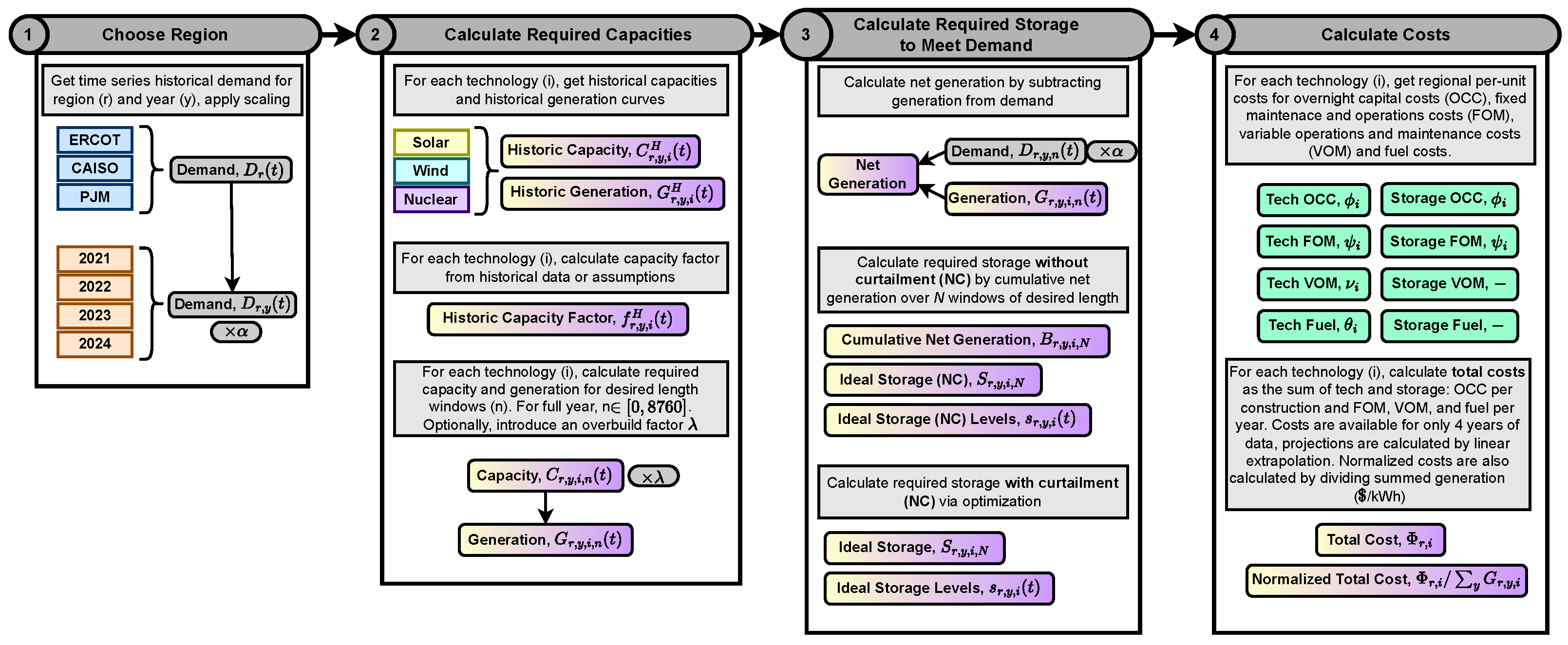
In the methodology for calculating the BYOBattery metric, outlined in Figure 1, a specific technology i (e.g., wind, solar, or nuclear) in region r is required to meet the hourly demand at time t by employing ideal storage, which does not consider any ramp rate constraints, energy losses, degradation, grid constraint, or curtailment. While ramp rate constraints, grid constraints, and energy losses would all act to increase the actual storage requirement relative to the BYOBattery estimate; however, for the same type of the battery assumed in BYOBattery, these impacts would be ignored. This conservative bias applies equally across all three technologies, so the relative ranking remains valid even under unrealistic assumptions.

The matching, or mismatching, of energy supply and demand is calculated across several years of data; the specific years are collected in the set $\mathbb{Y}$, where a given year $y\in \mathbb{Y}$. Data from each year are given in hourly integer time steps t such that, assuming no leap days, $t\in \mathbb{H}$, where $\mathbb{H}=[0,8760]\subset \mathbb{Z}$ for each year y. Additionally, it is helpful to define time windows by using different units of resolution (e.g., days, weeks, months). If N is the number of time windows per year, then a set ${\mathbb{T}}_n\subset \mathbb{H}$, where $n\in [0,N-1]$, contains the hourly indices for that time window n. For example, $N=52$ if the resolution is in weeks, and $N=8760$ if in hours.

The ideal battery storage requirement $S_{r,i,y,N}^{ideal}$ [GWh] for a specific time window n is defined as the imbalance between the maximum and minimum cumulative net generation:

$$S_{r,i,y,N}^{ideal}=max{B}_{r,i,y,N}-min{B}_{r,i,y,N}.$$

(1)

The cumulative difference, $B_{r,i,y,N}$, between the demand and generation is defined as:

$$B_{r,i,y,N}=\sum _{n=0}^N(D_{r,i,y,n}-G_{r,i,y,n}),$$

(2)

where $D_{r,i,y,n}$ [GW] is the demand and $G_{r,i,y,n}$ [GW] is the generation for technology i during time window n. The demand time series that each technology i must fulfill in region r for time window n was calculated based on the historical data from the specific region (e.g., CAISO, ERCOT, PJM), as per:

$$D_{r,i,y,n}=\alpha \mathbb{E}\left[D_{r,y}^H\left(\tau \right)|\tau \in {\mathbb{T}}_n\right]\equiv \alpha {\mathbb{E}}_n\left[D_{r,y}^H\left(t\right)\right],$$

(3)

where ${\mathbb{E}}_n[·]$ is the expected value operator, defined in this case as representing the average value of the time series over a given time window n. If $N=8760$, then $n=t$ and:

$$D_{r,i,y,t}=\alpha D_{r,y,t}^H,$$

(4)

where $D_{r,y}^H\left(\tau \right)$ is the historical demand in region r at time $\tau$; the complete dataset is defined as $D_{r,y}^H\left(t\right)\forall \tau \in \mathbb{H}$. While the data here are in hourly time steps, they may also be presented in time steps of minutes or seconds, depending on the data sources. The parameter $\alpha =0.25$ was utilized in this study for demonstration purposes, so as not to bias the demands for a specific technology. In other words, each technology was assumed to fulfill an equal portion of the full demand.

The generation curves $G_{r,i,y,n}$ for the different technologies were determined first by defining the capacity factor of electricity production from historical data, as shown in Equation (5). The capacity factor (dimensionless) is defined as:

$$f_{r,i,y,n}^H={\mathbb{E}}_n\left[{\displaystyle \frac{G_{r,i,y}^H\left(t\right)}{C_{r,i,y}^H\left(t\right)}}\right].$$

(5)

In Equation (5), $G_{r,i,y}^H\left(t\right)$ is the historical hourly actual energy output of the technology i, $C_{r,i,y}^H\left(t\right)$ is the historical hourly installed capacity of the technology i, and $f_{r,i,y,n}^H$ is the capacity factor per time window n, using historical data. Per this capacity factor definition, the technology capacity can be estimated as:

$$C_{r,i,y,N}=\lambda \mathbb{E}\left[{\displaystyle \frac{D_{r,i,y,n}}{f_{r,i,y,n}^H}}|n\in [0,N]\right],$$

(6)

where $C_{r,i,y,N}$ is the ratio of the desired demand to be met by each technology, over the mean capacity factor for the number of time windows of interest (N). If for a full year, a singular technology capacity is calculated across $N=8760$ time windows (this is the case for the majority of the analysis provided in Section 4, Section 5 and Section 6), an additional factor $\lambda$ is provided to augment the capacity, or overbuild the generation asset, past the initial estimate. However, by default it is equal to 1. With these normalization steps, the actual generation for each technology i in a given region r is:

$$G_{r,i,y,n}=f_{r,i,y,n}^H{C}_{r,i,y,N},$$

(7)

where the historical capacity factor values for the technology i in region r are combined with the estimated technology capacity $C_{r,i,y,N}$ required to meet the average regional demand (assuming $\lambda =1$). Later, the amount of overbuilding of the technology capacity is compared against adding new storage capacity: increasing $\lambda$ affects the cumulative net generation and thus the ideal storage requirement $S_{r,i,y,N}^{ideal}$.

Temporal, region-specific generation and demand data are required for analyzing the total required ideal storage. Depending on the need for analyzing the energy characteristics in different regions/years, daily, weekly, monthly, or yearly battery installation storage capacities can be shown. For example, in the present research, $C_{r,i}^H\left(t\right)$ was collected from the selected regions and years in quarterly, monthly, or hourly resolution. $G_{r,i}^H\left(t\right)$ for wind and solar was in hourly resolution. Meanwhile, $G_{r,i}^H\left(t\right)$ for nuclear was assumed to operate at 100%. A detailed data representation is given in Section 3.1

2.2. Bring Your Own Battery, with Curtailment

In practice, excess generation should be curtailed if the storage level exceeds the necessary minimum capacity required to match demand. The authors formulated this storage-with-curtailment problem as an optimization problem that assumes perfect foresight by incorporating complete time-series data (e.g., an entire year) into its decision-making process. The perfect foresight assumption is a simplification that may cause differences in power generation and anticipated demand during real-time operations. However, it has been shown that simulations using perfect information differ by a small percentage (4–9%) from point forecast models [18]. Nevertheless, improvements from rolling optimization techniques and forecast models is a topic for future work. The time-dependent storage level, $s_{r,i}\left(t\right)$, is defined as:

$$s_{r,i}\left(t\right)=\eta ·s_{r,i}(t-1)+G_{r,i}\left(t\right)-D_{r,i}\left(t\right)-Cu{r}_{r,i}\left(t\right),$$

(8)

where $Cu{r}_{r,i}\left(t\right)$ is the amount of curtailment at time t. The battery efficiency ($\eta$) can be used to consider the degradation stemming from charging and discharging the battery, but for the type of ideal battery covered in this paper, $\eta =1$. The round-trip efficiency losses would increase real storage requirements but would not change the relative technology ranking.

The initial condition ($t=0$) is defined as:

$$s_{r,i}\left(0\right)=s_{r,i,initial}+G_{r,i}\left(0\right)-D_{r,i}\left(0\right)-C_0\left(t\right),$$

(9)

where $s_{r,i,initial}$ is the initial storage level at time $t=0$. For each time t, the storage level $s_{r,i}\left(t\right)$ cannot exceed the storage capacity $S_{r,i,max}$, which is set as the constraint of the optimization, the objective of which is to minimize the sum of the maximum storage required to fulfill the 230 time-dependent demand mismatch in the region, $S_{r,i,max}$. For simplicity, the initial storage level was assumed to be 100% full in the problem, though in actuality this amount will vary depending on the technology employed. A key benefit of this algorithm is that the feasible region of the optimization problem is convex, guaranteeing that any local minimum is also a global minimum and thus ensuring the convergence of the problems. Overall, the perfect foresight optimization algorithm presented in this section provides a rigorous, efficient approach to energy storage dispatch planning.

2.3. Total Cost Estimation for Battery and Installed Capacity

The total cost estimation considered in this paper encompasses two portions: the costs from the newly installed capacity and the costs from the required batteries, as shown in Equation (10):

$${\Phi }_{r,i}^{total}={\gamma }^{T}OC{C_{r,i}}^T+{\gamma }^{S}OC{C}_{r,i,y}^S+\left({\displaystyle \frac{Y}{\widehat{Y}}}\right)·\sum _{y=1}^{\widehat{Y}}\left(FO{M}_{r,i,y}^T+VO{M}_{r,i,y}^T+Fue{l}_{r,i,y}^T+FO{M}_{r,i,y}^S\right),$$

(10)

where the technology costs (denoted by the superscript T) include $OC{C}_{r,i}^j$ the yearly overnight capital costs (OCC), [$/kW], $FO{M}_{r,i,y}^j$ the fixed operation and maintenance costs (FOM) [$/kW-yr], $VO{M}_{r,i,y}^j$ the variable operation and maintenance costs (VOM) [$/MWh], and $Fue{l}_{r,i,y}^j$ the fuel costs [$/MWh] for the corresponding region ($r=[0,1,2]$ for CAISO, ERCOT, PJM) and technology ($i=[0,1,2]$ for solar, wind, nuclear). Note that for the superscript j, $j=S$ represents battery costs while $j=T$ represents technology costs for the corresponding technology in the subscript i. The battery costs (denoted by the superscript $j=S$) include overnight capital and FOM costs. The non-capital costs are summed over $\widehat{Y}$ years of available data, but can be extrapolated to a projected cost over Y years if $Y>\widehat{Y}$. The OCC for technologies and storage are further modified by a parameter ${\gamma }^j$:

$${\gamma }^j=\left\{\begin{array}{c}1+⌊{\displaystyle \frac{Y-1}{L_s}}⌋,\mathrm{for}j=S\hfill \\ 1+⌊{\displaystyle \frac{Y-1}{L_i}}⌋\mathrm{for}j=T.\hfill \end{array}\right.$$

(11)

This parameter adds a new construction cost if the lifetime L in years is less than the project lifetime Y (that is, the component must be rebuilt). This approach addresses some of the imperfect battery where the component lifetime is shorter than the project lifetime. In such a case, a simplifying assumption is made that the rebuild occurs immediately. Note that only nuclear carries the VOM and fuel costs, while solar and wind do not. The overnight capital, FOM, VOM, and fuel costs are all calculated as shown in Equations (12)–(14):

$$OC{C}_{r,i}^j=\left\{\begin{array}{c}{\varphi }_s{S}_{r,i,y,N}^{ideal},\mathrm{for}j=S\hfill \\ {\varphi }_i{C}_{r,i,y,N}\mathrm{for}j=T,\hfill \end{array}\right.$$

(12)

where ${\varphi }_i$ is the unit overnight capital costs (OCC) for building an entire new technology i with capacity $C_{r,i,y,N}$, and ${\varphi }_s$ is the unit OCC for building battery storage with capacity $S_{r,i,y,N}^{ideal}$. No economies of scale were considered for the study, which would make these scalings nonlinear. In fact, more economic benefits for all the technologies are obtained when more constructions are built in the near future. This effect will be considered in future research.

Similar equations can be shown in Equation (13) but overnight capital is replaced with FOM.

$$FO{M}_{r,i,y}^j=\left\{\begin{array}{c}{\psi }_s{S}_{r,i,y,N}^{ideal},\mathrm{for}j=S\hfill \\ {\psi }_i{C}_{r,i,y,N}\mathrm{for}j=T.\hfill \end{array}\right.$$

(13)

For nuclear technology VOM and fuel cost estimation, Equation (14) was used, where ${\nu }_i$ can be the unit costs of either VOM or the fuel, while $g_{r,i,y}\left(t\right)$ is the amount of nuclear generation with curtailment, based on the estimation from Section 2.2.

$$v_{r,i,y}^j=\left\{\begin{array}{c}0,\mathrm{for}j=S\hfill \\ 0,\mathrm{for}j=T\wedge i\in \{0,1\}\hfill \\ {\nu }_i{g}_{r,i,y}\left(t\right)\mathrm{for}j=T\wedge i=2.\hfill \end{array}\right.$$

(14)

The total fuel costs for nuclear are assumed to scale linearly with the generation amount. This is common practice in nuclear cost modeling, as actual marginal fuel cost curves are often reactor-specific, much more complex to accurately incorporate into these simple models, and require business proprietary information [19].

3. Data Acquisition

The data required in the BYOBattery analysis are collected for two purposes: (1) BYOBattery analysis to answer the research question of how many batteries would be required in various regions in the United States, and (2) cost analysis to find the optimized costs based on the minimum storage size for each technology. Section 3.1 visualizes the nameplate capacity, generation, and demand data for the specified technology in multiple regions and years. Section 3.2 documents the overnight capital, FOM, variable operation, VOM, and fuel costs for each specified technology.

3.1. Technology Characterization for Multiple Regions and Years

For demonstration purposes, the technologies of interest are wind, solar, and nuclear. Wind and solar are intermittent sources whose generation profiles are independent of the demand profiles. Nuclear energy, however, usually serves as baseload generation, providing steady power for a non-steady demand profile. Therefore, for all three technologies, battery size was estimated by applying the BYOBattery method. As shown in Section 2, the historical installed capacity, generation profiles, and demand profiles for each technology are required. The regions of interest are CAISO, ERCOT, and PJM. For each region, the historical data on each technology for the years 2021 to 2024 [20,21,22] were extracted from publicly available websites. For solar and wind, the capacity factors were calculated via the ratio of the generation over the installed capacity. For nuclear, the generation was assumed to be identical to the nameplate capacity for each region. For light water reactors, the averaged capacity factor is 93% [23]. Advanced nuclear reactors such as Xe-100 and KP-FHR have the feature of online refueling so that the capacity factor can approach 100%. The assumption of 100% capacity in this paper is an ideal situation for demonstrating the BYOBattery metrics.

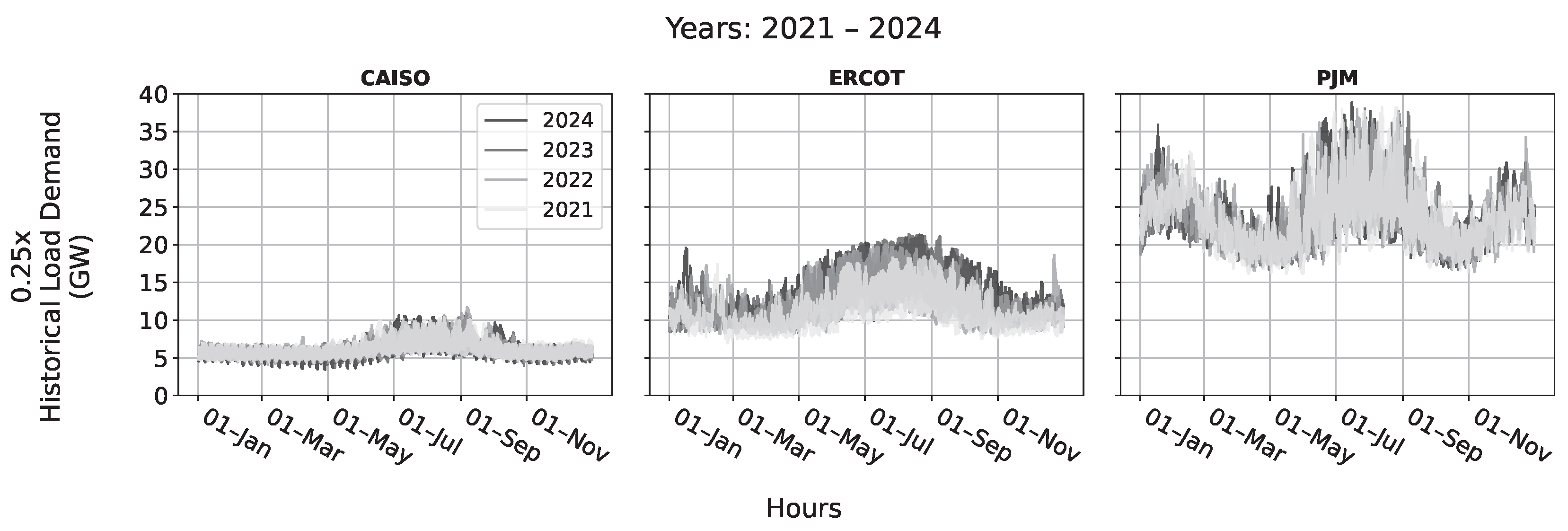
Figure 2 visualizes the hourly demand, using a factor of 0.25 to account for the proportion of demand to be met by each technology in CAISO, ERCOT, and PJM during the period of 2021 to 2024. In the figure, CAISO shows a signal peak in load demand during late summer—specifically between July and September. Similarly, ERCOT displays this pattern, but in comparison with CAISO, it also has a more distinct peak in the winter months from December to March. PJM experiences both summer and winter peaks, with the summer peak being slightly more significant than the winter one. Additionally, PJM has more noticeable dips in demand during the spring and fall.

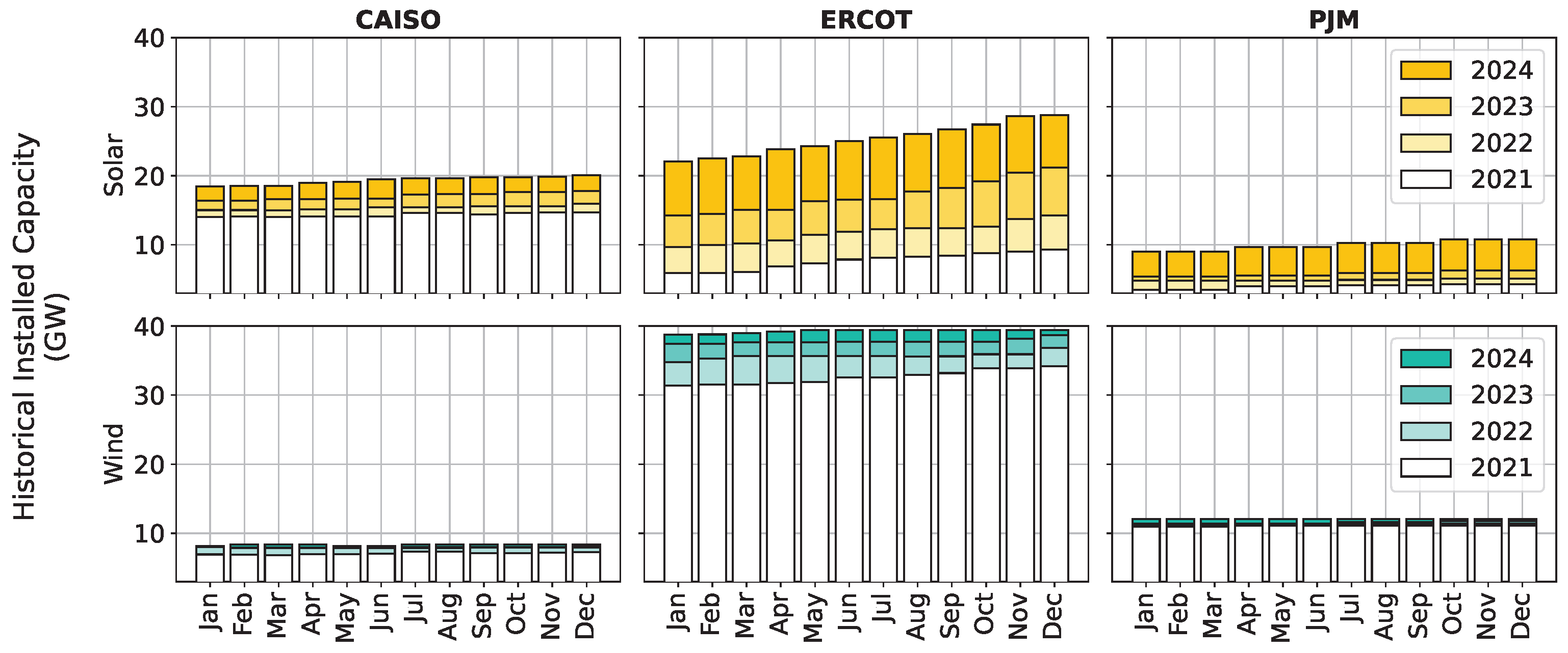
Figure 3 and Figure 4 report the installed capacity and capacity factor for wind and solar, respectively, in CAISO, ERCOT, and PJM between 2021 to 2024. Per Figure 3, solar energy has seen increased growth in ERCOT and PJM. Conversely, CAISO had a larger amount of existing solar generation in 2021 as compared with the following years. In contrast, wind energy has not grown much in these regions, given that ERCOT already installed wind capacity over 30 GW prior to 2021.

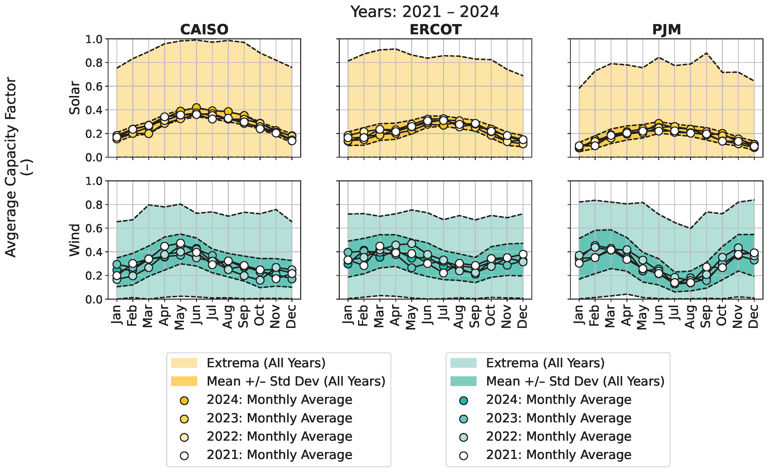
For Figure 4, the hourly generation and demand data were resampled to show the monthly time series in tandem with the monthly averages, one standard deviation, and a monthly extrema envelope about those averages. The solar generation peaks during the summer are more pronounced across the regions. ERCOT exhibits higher wind generation in the first half of the year, whereas CAISO reaches its peak around May. PJM displays dual seasonal peaks, with peak wind generation occurring in early spring and late fall, and with a significant trough during the summer.

3.2. Cost Data for Multiple Technologies

The costs required for economic assessment include the overnight capital, FOM, and VOM costs. For nuclear technology, the fuel costs are typically separated from the FOM or VOM costs. The authors utilized cost data from the 2024 Annual Technology Baseline (ATB) developed at the National Renewable Energy Laboratory [24], and converted them into the 2025 cost values, as shown in

Table 1. Cost values from the National Renewable Energy Laboratory 2024 ATB, as escalated to 2025 USD.

Technology	Lifetime	OCC	FOM	VOM	Fuel
Solar	30 yr	$1476/kW	$26/kW-yr	$0/MWh	$0/MWh
Wind	30 yr	$1590/kW	$35/kW-yr	$0/MWh	$0/MWh
Nuclear	80 yr	$8640/kW	$147/kW-yr	$3/MWh	$12/MWh
Storage	15 yr	$461/kWh	$12/kWh-yr	$0/MWh	$0/MWh

.

As shown in Table 1, solar and wind share a similar unit cost of overnight capital and VOM, while nuclear actually has the highest overnight capital and FOM costs by comparison. NPPs have unique VOM and fuel costs but are not necessitated by solar, wind, and storage facilities. However, nuclear also offers the longest operational lifetimes. Therefore, Section 5 will discuss the overall cost profile when considering the generation, capacity demands, and lifetime of the technology.

4. Temporal and Region-Specific BYOBattery Analysis

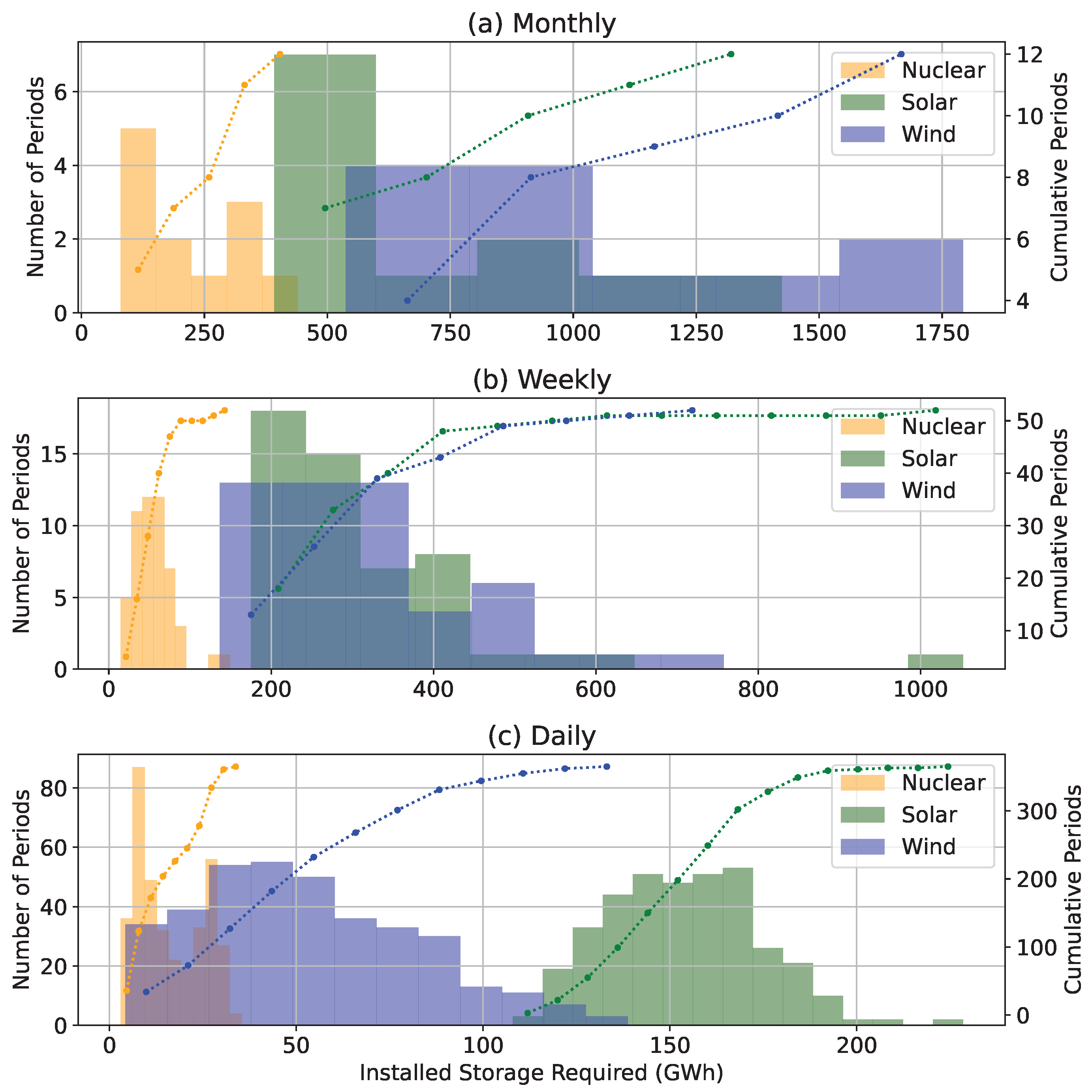
The simplest representation of the BYOBattery is to demonstrate the daily, weekly, or monthly ideal battery storage requirements in units of GWh before any consideration of curtailment, as demonstrated in Section 2.1. For example, Figure 5 shows a histogram of the monthly, weekly, and daily ideal storage requirements for ERCOT in 2023. In Figure 5a, the bins represent the storage amount needed to meet the generation-demand imbalance with 25% of demand for each different time window length (e.g., the average in each month, week, or day), and the frequency values then represent the number of time windows in a year that require that minimum storage. For example, in 2023, there are five months in which the nuclear technology needs ≥250 GWh of ideal battery storage, four months in which the solar technology needs ≥750 GWh, and three months in which the wind technology will require ≥1250 GWh. Note that the storage requirements in Figure 5 do not consider continuity between time windows; that is addressed when curtailment is modeled, where the time window selected is a full year. Based on Figure 5a,b, the ideal battery storage distributions overlap, making it difficult to differentiate which technology needs more battery storage. However, for daily representations, it is apparent that solar needs more battery storage in comparison with wind technology. Regardless of whether talking about the daily, weekly, or monthly representation, nuclear generation needs the smallest amount of battery storage in comparison with wind and solar. This observation aligns with the practice that nuclear generation is served as the steady base load while wind and solar show intermittent profiles where regional variations are significant.

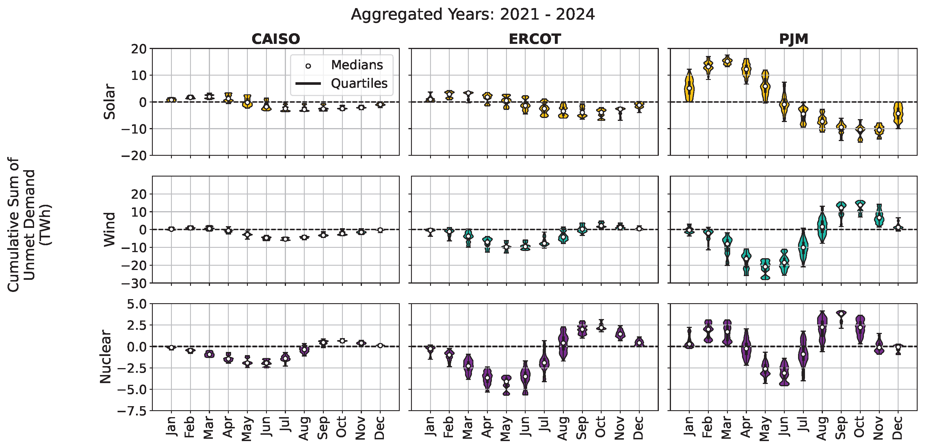
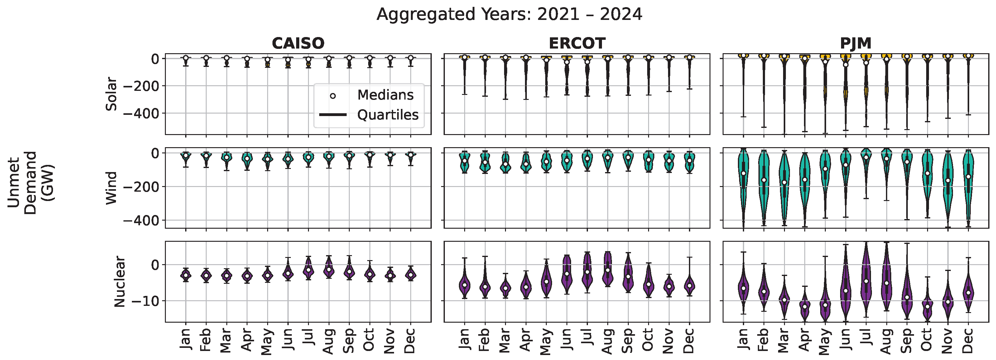
In practice, the amount of curtailment should be considered when estimating the ideal battery storage requirement. To facilitate this estimation, it is critical to know when the demand is unmet and when the generation is overproduced. Figure 6 shows the cumulative sum of the unmet demand for CAISO, ERCOT, and PJM from 2021 to 2024. As a general trend, the unmet demand for solar has peaks during the winter and early spring, while the wind has a peak during the summer and fall. Figure 6 demonstrates the annual fluctuations in the cumulative sum of demand, also termed the total idealized storage dispatch. The positive unmet demand indicates the amount of ideal battery storage required, while the negative unmet demand refers to the amount of curtailment required for each technology. As expected, solar energy experiences its most pronounced deficits in the early part of the year, particularly during the winter months. This trend is consistently observed across all three regions of the United States, although the severity varies in each. The reduction in solar irradiance and the shorter daylight hours during winter decrease solar energy production, thereby increasing dependence on storage solutions to meet demand. Conversely, wind and nuclear energy display distinct storage requirement patterns at different times throughout the year. In late summer and early fall, both wind and nuclear energy technologies encounter more significant deficits than in other periods. This phenomenon may be linked to seasonal transitions, with changes in weather patterns and regional factors affecting the availability and consistency of wind and nuclear energy generation. For example, variability in wind speeds and potential planned maintenance outages for NPPs during the fall could contribute to increased storage demands.

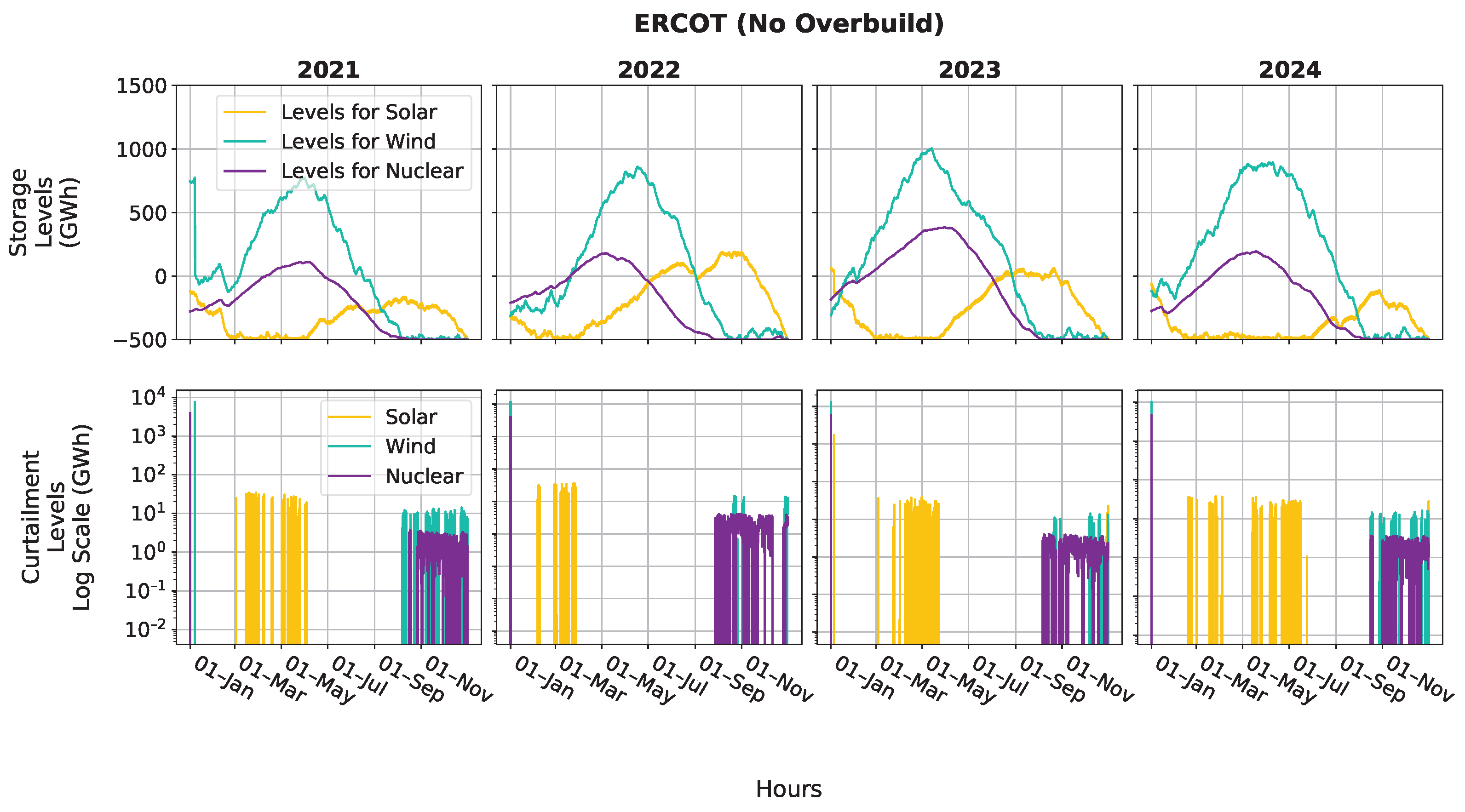
Based on the unmet demand curves, it is possible to decouple the figures into positive unmet demand (ideal battery storage level) and negative unmet demand (curtailment level). Figure 7 breaks down the ideal battery storage and curtailment level in ERCOT from 2021 to 2024.

Between 2021 and 2024, nuclear energy exhibited the most stable storage dispatch, with charging predominantly occurring during the early part of the year. In contrast, wind and solar energy demonstrated greater variability, as characterized by rapid charge-discharge cycles. Regarding storage requirements, wind energy necessitated the most substantial battery storage capacity, up to 15,000 GWh, regardless of year. Solar energy, on the other hand, required approximately 5000 GWh of ideal battery storage. On average, nuclear energy necessitated slightly more storage than did solar energy in this region of the United States.

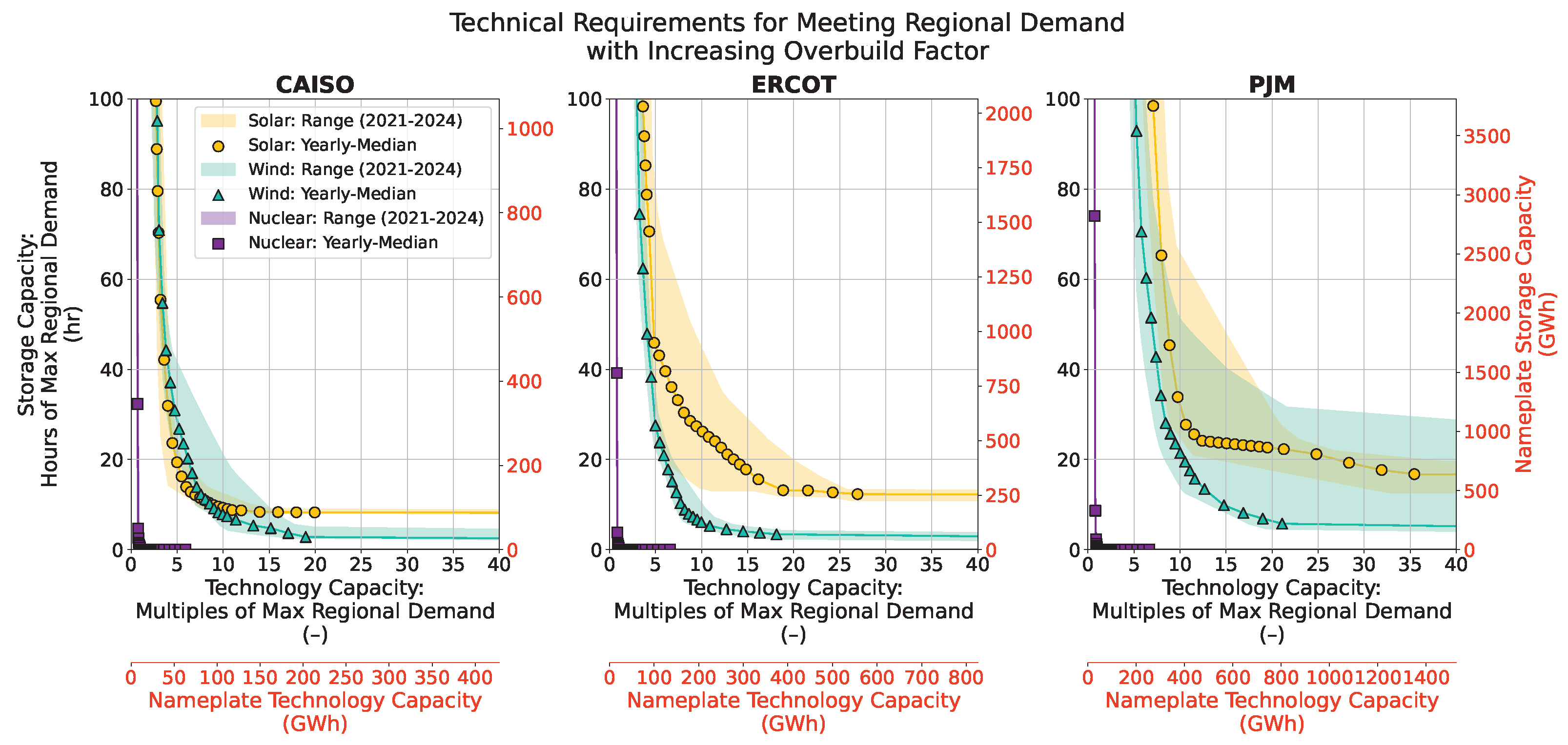
Figure 8 considers the relationship between installed generation and ideal battery storage requirements for each individual technology. Each graph represents a specific region, and the spread about the curve represents the variety of outcomes across multiple years in the 2021–2024 range. On the x-axis is the amount of generation capacity installed to meet demand, and on the y-axis is the amount of ideal battery storage required to balance the mismatch between generation and demand. As expected, as generation increases, the amount of storage required decreases. Of particular interest is the rapid drop in storage required for nuclear generation, suggesting that regardless of the region or year considered, building additional nuclear capacity rapidly diminishes the amount of storage required to offset supply-demand mismatches. Of the three regions, PJM has the highest storage requirement given the same generation capacity.

5. Economic Assessment for Estimating the Cost of Storage

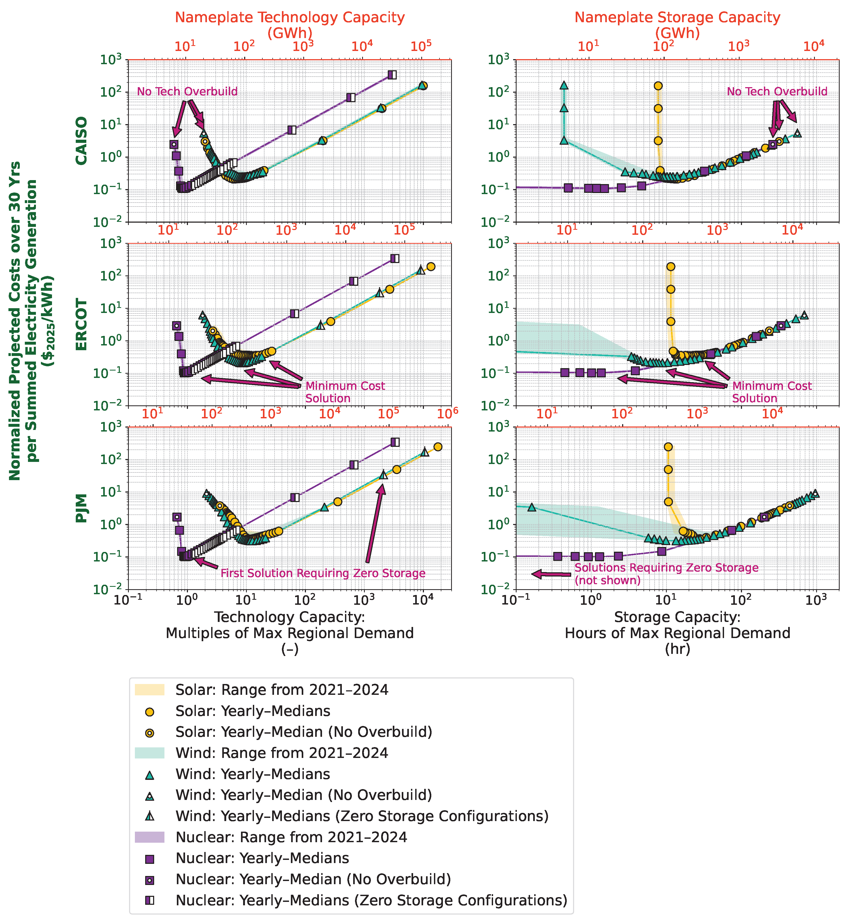
The economic assessment in this paper focuses on comparing the total costs (in units of billion USD), including the technological contribution (i.e., solar, wind, or nuclear) and ideal battery storage contribution. All the costs are linearly summed so as to compare the original costs without considering the discounted rate or amount of inflation that will be incurred over the next 30 years. Based on the lifetime reported in Table 1, the OCC for wind, solar, and nuclear are considered once, while storage costs are considered twice. Figure 9 shows the cost curve as a function of nameplate capacity (on the left) and storage capacity (on the right) for CAISO, ERCOT, and PJM during the period of 2021 to 2024. These costs are normalized by the summed electricity generation over 30 years.

The data points in Figure 9 represent the median values throughout all the years on a logarithmic scale, with the shaded envelopes indicating the range of yearly values. Recall from Figure 8 that low technology capacities require large amounts of storage, and that as more technology capacity is added, the required storage amount decreases. Figure 9 is a continuation of the previous figure, but highlights the resultant costs. The data are arranged in a 3 × 2 grid of plots, with the various rows pertaining to different regional results. The left-hand column shows the normed cost trending with increasing technology capacity, while the right-hand one shows those same costs but trending with increasing storage capacity. Each cost data point pertains to a pair of technology and storage capacities, so each row shares the same y-axis. The right column therefore reads from right to left in order of the data points. Each subplot shows the costs for the three technologies. As a general trend for each technology, the total costs are initially reduced when each technology’s nameplate capacity increases. The increased nameplate capacity of the specific technology can reduce the amount of required storage (i.e., reverse order [from right to left] in the x-axis). When each technology’s nameplate capacity reaches a certain point, the total cost starts to increase. This leads to the lowest cost being observed in the left-hand subplots. This behavior can be interpreted as indicating that the storage capital costs dominate the total OCC when the nameplate capacity is small (i.e., to the left of the minimum), while the technology capital costs dominate when the nameplate capacity is high (i.e., to the right of the minimum). A minimum cost for nuclear is observed to occur at much lower technology capital costs than for the other two technologies, as nuclear technology requires less storage. In comparing the total costs from multiple regions, PJM has the highest minimum points and CAISO the lowest.

In the right-hand subplots of Figure 9, a sharp cost increase is observed when the technology capital costs surpass the storage capital costs. For wind and solar energy technologies, which reflect zero values at certain points within a given year, the storage requirements remain constant because they have already achieved the minimum storage needed to meet demand, which is always non-zero. In contrast, nuclear storage requirements decrease to zero as the technology capacity increases. In regions such as ERCOT and PJM, extended shaded areas are observed for wind technology, which reach zero as the nameplate capacity increases. This increase is due to continuous generation throughout the year for nuclear and wind in these regions, resulting in minimal need for additional storage installation.

Table 2. Minimum costs for each technology and coupled storage system for all regions. Averages over the 2021–2024 results are provided for each column along with standard deviation from data variability.

Region-Technology	OCC (Technology) B$2025	OCC (Storage) B$2025	30-Yr Summed Costs B$2025	30-Yr Summed Costs per Electricity Generated B$2025/kWh
CAISO-Solar	97.45 ± 18.17	137.10 ± 12.53	337.30 ± 20.34	0.21 ± 0.02
CAISO-Wind	165.30 ± 36.57	99.84 ± 29.78	410.39 ± 70.36	0.26 ± 0.04
CAISO-Nuclear	78.72 ± 4.39	14.41 ± 1.49	171.38 ± 8.60	0.11 ± 0.00
ERCOT-Solar	377.21 ± 137.69	337.94 ± 98.07	1040.55 ± 257.00	0.32 ± 0.08
ERCOT-Wind	282.13 ± 15.88	148.89 ± 18.41	670.86 ± 51.13	0.21 ± 0.02
ERCOT-Nuclear	156.05 ± 10.01	25.30 ± 1.45	335.26 ± 21.19	0.10 ± 0.00
PJM-Solar	792.20 ± 208.12	863.03 ± 84.00	2396.11 ± 412.59	0.38 ± 0.07
PJM-Wind	786.29 ± 130.84	692.69 ± 435.85	2251.53 ± 720.50	0.36 ± 0.11
PJM-Nuclear	298.44 ± 2.78	45.82 ± 4.47	637.64 ± 5.78	0.10 ± 0.00

presents the minimum costs for each technology in the different regions, accounting for the uncertainty that exists throughout the period of 2021 to 2024.

In Table 2, the solar storage capital costs exceed the technology capital costs across all regions, while the nuclear technology costs exceed the nuclear storage costs. This discrepancy is likely due to the different orders of magnitude of the ranges when comparing solar, nuclear, and their coupled, optimally sized storage systems. Wind technology capital costs exceed storage costs in CAISO and ERCOT but not in PJM. PJM tends to have the highest technology cost and storage costs compared with the other region due to higher demand and storage requirement. Summed 30-year costs, which also include reconstruction costs for storage, FOM, VOM, and fuel costs, range between hundreds of billions of USD to nearly 2.5 trillion USD. These enormous costs stem from the assumption that all the technologies will be built from the ground up, starting from zero existing portfolios which is not the current reality. Rather, these cost values should be used for comparisons only. To normalize these values and facilitate comparisons, they are provided in USD per kWh of electricity generated, in the final column of Table 2. Here, wind and solar costs range between 0.20 and 0.38 USD per kWh across all regions, while nuclear costs are close to 0.10 USD per kWh. The cost of the nuclear matches the moderate LCOE estimation from [24]; however, it is important to note that these cost estimates do not include any land area or land-usage costs and should be considered as a relative cost for each technology.

6. Optimized Storage-Informed Dispatch

By combining the technological requirements for storage and economic cost estimations (see Section 5 and Section 6), the optimal values for storage-coupled technology systems were evaluated.

Table 3. Optimal technology and storage sizes, based on projected 30-year costs. Averages over the 2021–2024 results are provided for each column, with standard deviation.

Region-Technology	Demand for Sizing (GW)	Optimal Nameplate Capacity (GW)	Optimal Storage (GWh)	Equivalent Load Hours of Storage (hr)	Number of Discrete Storage Units Required
CAISO-Solar CAISO-Wind CAISO-Nuclear	Mean: 6.00–0.11 Max: 10.87–0.51	66.01 ± 12.31 103.98 ± 23.01 9.11 ± 0.51	148.55 ± 13.58 108.17 ± 32.26 15.61 ± 1.61	13.65 ± 0.74 9.89 ± 2.72 1.44 ± 0.16	249.00 ± 23.00 181.00 ± 54.00 27.00 ± 3.00
ERCOT-Solar ERCOT-Wind ERCOT-Nuclear	Mean: 12.33–0.71 Max: 20.27–1.20	255.50 ± 93.26 177.47 ± 9.99 18.06 ± 1.16	366.15 ± 106.26 161.31 ± 19.95 27.41 ± 1.57	17.86 ± 4.46 7.97 ± 0.96 1.35 ± 0.02	611.00 ± 177.00 270.00 ± 34.00 46.00 ± 3.00
PJM-Solar PJM-Wind PJM-Nuclear	Mean: 23.80–0.22 Max: 38.27–0.36	536.59 ± 140.97 494.59 ± 82.30 34.54 ± 0.32	935.05 ± 91.01 750.50 ± 472.23 49.65 ± 4.85	24.43 ± 2.41 19.50 ± 12.04 1.30 ± 0.12	1559.00 ± 152.00 1252.00 ± 787.00 84.00 ± 9.00

shows the demand for sizing of the technology, optimal nameplate capacity, optimal storage, equivalent load hours of storage, and number of discrete storage units required for each storage-coupled technology.

The parameters in Table 3 were chosen based on the minimized 30-year projected costs shown in Table 2. Each tabulated entry represents an average value across all the years comprising 2021 and 2024, with an additional standard deviation also being provided. These metrics were categorized by region as well as by the technology mixes within each region. The mean and maximum demand levels per region are shown for comparison. These demand values are used for sizing, and have been scaled down by a factor of 4. The average and maximum of these scaled demand levels were calculated per year; the average of each of those metrics across all years is provided, along with a standard deviation. The optimal nameplate capacity for wind and solar, regardless of region, span an order of magnitude higher than the average demand for the region. For nuclear, however, the optimal nameplate capacity ranges somewhere between the mean and maximum demand level. The corresponding optimal storage shows a similar trend in which solar needs the highest amount of storage, followed by wind and nuclear.

The cost-optimal storage in Table 3 is represented in three different ways. The first is via the nameplate capacity in GWh. The second is by normalizing the storage capacity by the maximum load experienced in each region. This results in the equivalent load hours of storage in units of hours. Finally, the storage capacity can also be normalized by assuming a standard unit size of battery storage, then calculating the number of discrete storage units required to efficiently match the regional demand mismatch. The largest unit of the battery storage in the ATB [24] was used, along with the corresponding costing data. This was a utility-scale battery storage with 60 MW power outputs and 10 h of charging capabilities, for a storage capacity of 600 MWh.

The optimal amount of storage required for wind and solar is equivalent to 9–14 h of equivalent load hours in CAISO. Solar-coupled storage requires energy equivalent to approximately 18 h of equivalent load-hour operations in ERCOT, while wind requires only about 8 h of storage. In PJM, solar and wind require much larger amounts of storage, equivalent to 20–25 h of PJM maximum load. Nuclear, regardless of region, requires storage equivalent to about 1 h of maximum load operations in each region (though the energy requirements will differ across regions). This is an order of magnitude lower than the requirements of solar and wind across all regions.

In comparing the number of discrete energy storage units, we see that several hundred are required in CAISO and ERCOT for wind and solar, while nearly 1500 units are needed in PJM for wind and solar. Nuclear requires 30 energy storage units for CAISO, about 49 for ERCOT, and nearly 93 for PJM—when including the upper bound standard deviation about the mean.

Using the optimal nameplate capacity, the unmet demand curve can be updated as shown in Figure 10.

In Figure 10, the unmet demand for solar across the months exhibits a distribution in the positive y-axis, corresponding to nighttime unmet demand. However, the amount of the unmet demand is significantly reduced as compared with those shown in Figure 6. A similar trend is observed for wind and nuclear, with the median values being shifted from positive to negative if optimal technology capacity is applied. The plots in Figure 6 and Figure 10 only consider technology capacity without storage. Comparing Figure 10 with Figure 6 shows that the decreased unmet demand results in lower storage capacity requirements while also necessitating curtailment due to increased overproduction. For wind, the median unmet demand is lowest (i.e., highest overproduction) near mid-spring for CAISO. Similar trends are evident in ERCOT and PJM, with a sharp decrease in overproduction between July and August resulting in larger distributions of unmet demand. The nuclear unmet demand distributions more closely align with the demand profile for monthly distributions.

7. Conclusions

In conclusion, development of the BYOBattery method effectively addressed the key research question concerning the optimal number of batteries and total capacity of battery storage needed to meet demand across the different regions, considering both existing and potential increases in nameplate capacity. The amount of storage required by individual technologies can be used for regional comparison studies so as to ascertain the technologies’ effectiveness and resilience when deployed in electricity grids. The results from the BYOBattery analysis will help inform subsequent, more detailed studies on capacity planning. With these comparison metrics, stakeholders can make informed decisions, leading to efficient resource usage, improved energy resilience, and lower energy costs. This study demonstrates the fact that the BYOBattery algorithm, particularly with curtailment, significantly reduces the constraints posed by maximum generation peaks, and highlights the critical sensitivity to mean reversion.

The key findings are as follows:

• Introduction of additional curtailable nuclear generation drastically reduces the amount of energy storage required to meet the demand profiles.
• Both wind and solar technologies require a certain level of storage—even without consideration of curtailment—in most of the regions and years covered. In ERCOT and PJM, the required amount of storage can approach zero when the nameplate capacity is large enough (on the order of 100 terrawatts).
• Nuclear generation consistently requires less storage compared with wind and solar regardless of consideration for curtailment. Nuclear technology is the cost-optimal option, with the storage needs totaling approximately one equivalent load hour, as compared with the significantly higher storage requirements for wind and solar. The optimal installed generation capacity for nuclear is lower across all regions than for wind and solar.
• The variation in storage requirements across regions highlights the importance of region-specific analyses, with PJM showing the highest demand variability.
• The cost analysis reveals that the 30-year non-discounted cost per kWh for nuclear generation is approximately $0.10, which is lower than the wind or solar generation costs by a factor of 1–4. These findings underscore the potential for nuclear generation to play a pivotal role in achieving cost-effective and reliable energy storage solutions.

Future research will target relaxing the ideal battery assumption so as to consider degradation of the battery during charging and discharging cycles. Additionally, the impact of the economies of scale with the learning curve of new technology deployment will be considered. Also, the power supply reliability for each technology can be served as another objective function for optimization in addition to cost, leading to a multi-objective optimization research. The realization of non-ideal storage can consider standby losses, which are crucial for long-duration analyses (e.g., weekly, monthly, and yearly). To adopt this methodology for location specific decision-making process, a comprehensive sensitivity and uncertainty quantification is required to capture and ranges of the BYOBattery metric estimation. The real cost value should be benchmark with a real construction project as part of the future work.

References

1. Davenport, C.; Singer, C.; Mehta, N.; Lee, B.; Mackay, J. AI, Data Centers and the Coming US Power Demand Surge; Goldman Sachs: New York, NY, USA, 2024; p. 26. [Google Scholar]
2. White House. Unleashing American Energy. Available online: https://www.whitehouse.gov/presidential-actions/2025/01/unleashing-american-energy/ (accessed on 30 March 2026).
3. North American Electric Reliability Corporation. Characteristics and Risks of Emerging Large Loads-Large Loads Task Force White Paper; Technical Report; NERC: Washington, DC, USA, 2025. [Google Scholar]
4. Sodano, D.; DeCarolis, J.F.; de Queiroz, A.R.; Johnson, J.X. The symbiotic relationship of solar power and energy storage in providing capacity value. Renew. Energy 2021, 177, 823–832. [Google Scholar] [CrossRef]
5. Frazier, A.W.; Cole, W.; Denholm, P.; Greer, D.; Gagnon, P. Assessing the potential of battery storage as a peaking capacity resource in the United States. Appl. Energy 2020, 275, 115385. [Google Scholar] [CrossRef]
6. Mertens, T.; Bruninx, K.; Duerinck, J.; Delarue, E. Capacity credit of storage in long-term planning models and capacity markets. Electr. Power Syst. Res. 2021, 194, 107070. [Google Scholar] [CrossRef]
7. Wang, S.; Zheng, N.; Bothwell, C.D.; Xu, Q.; Kasina, S.; Hobbs, B.F. Crediting variable renewable energy and energy storage in capacity markets: Effects of unit commitment and storage operation. IEEE Trans. Power Syst. 2022, 37, 617–628. [Google Scholar] [CrossRef]
8. Qi, N.; Pinson, P.; Almassalkhi, M.R.; Zhuang, Y.; Su, Y.; Liu, F. Capacity Credit Evaluation of Generalized Energy Storage Considering Endogenous Uncertainty. arXiv 2024, arXiv:2406.07338. [Google Scholar] [CrossRef]
9. Pratama, Y.; Mac Dowell, N. Beyond LCOE: Value of Technologies in Different Generation and Grid Scenarios; Technical Report; IEA Greenhouse Gas R& D Programme (IEAGHG): Cheltenham, UK, 2020. [Google Scholar]
10. Phung, D.L. Cost Comparison Between Base-Load Coal-Fired and Nuclear Plants in the Midterm Future (1985–2015); Technical Report; Institute for Energy Analysis: Oak Ridge, TN, USA, 1976. [Google Scholar]
11. Kabeyi, M.J.B.; Olanrewaju, O.A. The levelized cost of energy and modifications for use in electricity generation planning. Energy Rep. 2023, 9, 495–534. [Google Scholar] [CrossRef]
12. Guo, W.; Fan, W.; Zhao, Y.; An, J.; He, C.; Guo, X.; Qian, Y.; Ma, L.; Zhao, H. Grouping Control Strategy for Battery Energy Storage Power Stations Considering the Wind and Solar Power Generation Trend. Energies 2023, 16, 1857. [Google Scholar] [CrossRef]
13. Arnaoutakis, G.E.; Kocher-Oberlehner, G.; Katsaprakakis, D.A. Criteria-Based Model of Hybrid Photovoltaic–Wind Energy System with Micro-Compressed Air Energy Storage. Mathematics 2023, 11, 391. [Google Scholar] [CrossRef]
14. Ahmed, A.; Massier, T. Techno-Economic Comparison of Stationary Storage and Battery-Electric Buses for Mitigating Solar Intermittency. Sensors 2023, 23, 630. [Google Scholar] [CrossRef] [PubMed]
15. Rogalev, N.; Rogalev, A.; Kindra, V.; Zlyvko, O.; Osipov, S. An Overview of Small Nuclear Power Plants for Clean Energy Production: Comparative Analysis of Distributed Generation Technologies and Future Perspectives. Energies 2023, 16, 4899. [Google Scholar] [CrossRef]
16. Matthews, J.; Bodel, W.; Butler, G. Nuclear Cogeneration to Support a Net-Zero, High-Renewable Electricity Grid. Energies 2024, 17, 6219. [Google Scholar] [CrossRef]
17. Meng, Q.; He, Y.; Gao, Y.; Hussain, S.; Lu, J.; Guerrero, J.M. Bi-level four-stage optimization scheduling for active distribution networks with electric vehicle integration using multi-mode dynamic pricing. Energy 2025, 327, 136316. [Google Scholar] [CrossRef]
18. Kahvecioğlu, G.; Morton, D.P.; Wagner, M.J. Dispatch optimization of a concentrating solar power system under uncertain solar irradiance and energy prices. Appl. Energy 2022, 326, 119978. [Google Scholar] [CrossRef]
19. Abou-Jaoude, A.; Lohse, C.S.; Larsen, L.M.; Guaita, N.; Trivedi, I.; Joseck, F.C.; Hoffman, E.; Stauff, N.; Shirvan, K.; Stein, A. Meta-Analysis of Advanced Nuclear Reactor Cost Estimations; Technical Report; Idaho National Laboratory (INL): Idaho Falls, ID, USA, 2024. [Google Scholar] [CrossRef]
20. California Independent System Operator (CAISO). CAISO-Home Page. Available online: https://www.caiso.com/ (accessed on 8 December 2024).
21. Electric Reliability Council of Texas (ERCOT). ERCOT-Home Page. Available online: https://www.ercot.com/ (accessed on 8 December 2024).
22. PJM Interconnection. PJM-Data Miner 2. Available online: https://dataminer2.pjm.com/feed/gen_by_fuel (accessed on 8 December 2024).
23. U.S. Energy Information Administration. Nuclear Explained: Nuclear Power Plants; U.S. Energy Information Administration: Washington, DC, USA, 2026. [Google Scholar]
24. National Laboratory of the Rockies. 2024 Annual Technology Baseline; Technical Report; National Laboratory of the Rockies: Golden, CO, USA, 2024. [Google Scholar]
Figure 1. Diagram of BYOBattery process.
Metrics 03 00008 g001
Figure 2. Historical demand averages per hour (with a factor of 0.25 to account for the proportion of demand to be met by each technology) across ERCOT, CAISO, and PJM (2021–2024).
Metrics 03 00008 g002
Figure 3. Historical nameplate capacity for solar and wind, per month, for ERCOT, CAISO, and PJM (2021–2024).
Metrics 03 00008 g003
Figure 4. Historical capacity factor averages, per month, for solar and wind across ERCOT, CAISO, and PJM (2021–2024).
Metrics 03 00008 g004
Figure 5. (a) Monthly, (b) weekly, and (c) daily bin histogram of the ideal battery storage requirement to meet 25% demand in ERCOT in 2023 without curtailment.
Metrics 03 00008 g005
Figure 6. Violin plots showing the distributions of the cumulative sums of unmet demand, by month of the year, across CAISO, ERCOT, and PJM (aggregated from 2021–2024).
Metrics 03 00008 g006
Figure 7. Required storage levels and curtailment of production for all technologies across the ERCOT region (2021–2024).
Metrics 03 00008 g007
Figure 8. Required storage capacity as a function of installed capacity per each technology for 2021–2024, as grouped by region. Note the different ranges in the y-axes.
Metrics 03 00008 g008
Figure 9. Total projected costs over a 30-year project, normalized by the summed electricity generation. Different regions are shown in log-scale on each row, grouped by technology and aggregated for 2021–2024. The left column shows the costs as a function of nameplate capacity; the right column shows the costs as a function of required storage.
Metrics 03 00008 g009
Figure 10. Violin plots showing the distributions of the cumulative sums of unmet demand after implementing optimal nameplate capacities for each technology, by month of the year, across CAISO, ERCOT, and PJM (aggregated from 2021–2024).
Metrics 03 00008 g010