Properties of Elliptic Cycloids

Abstract

Given an ellipse rolling along a straight line without slipping and a point P on the ellipse, we will determine the shape of the elliptic cycloid traced by P as the ellipse rolls and compute the area under one arch of the elliptic cycloid. We also investigate the arc length, though we are only able to express it as an integral.

1. Introduction

The family of curves known as cycloids have drawn interest for centuries (dating back to at least the 16th century) and arise naturally in a variety of physical settings. The most basic of the cycloidal curves is the circular cycloid, which is constructed by tracing the path of a point P on the circumference of a circle as the circle rolls along a straight line without slipping as illustrated in Figure 1.

If the given circle has radius r, then the area between one arch of the circular cycloid and the line upon which the circle rolls is $3\pi r^2$ (attributed to Galileo circa 1599 through experimental methods, and to Roberval and Descartes through mathematical proof in the 1630s as described in [1]) and the length of one arch is $8r$. These basic facts can be derived by first finding the parametric equations for the circular cycloid and are typically included in introductory calculus texts. The articles [2,3] (see also [4] for a more general construction) explore interesting variations using different shapes.

As mentioned, the circular cycloid arises naturally in certain physical settings. In particular, it is a solution to both the brachistochrone and tautochrone problems. The tautochrone is the frictionless curve with the property that a particle released from rest at any point on the curve takes the same length of time to reach the equilibrium point on the curve, whereas the brachistochrone is the frictionless curve which minimizes the travel time for a particle to reach an arbitrary point when projected from another point and constrained to live on the curve as described in [5]. The tautochrone problem was originally solved by Huygens in 1673 and the brachistochrone by Jean Bernoulli in 1697. See [5,6] for more on these problems and their generalizations. It is interesting to note that the circular cycloid solves both problems only when the particle in question is acted upon only by gravity; in the case of a general field of force, the problems yield distinct systems of curves. We also recommend Chapter 8 in [7] for an amusing tale involving Newton, Bernoulli and the brachistochrone.

Cycloids belong to the larger class of curves known as roulettes. These curves are defined in [8] as the locus of a point P that maintains a fixed position relative to a curve $\mathcal{C}$ as $\mathcal{C}$ rolls on another curve without slipping. For a general reference, we point the reader to [9] and for a shorter article containing a description of the parametric curves of certain roulettes, we point to [10]. The articles [8,11] provide an array of results on roulettes by utilizing the so-called “Roulette Lemma”.

For further reading, the article [12] describes a catenary as a roulette (rolling a parabola along a straight line and tracing its vertex). In [13], the author provides an interesting arc length identity for a limacon and uses this relationship to reproduce the arc length formula for a circular cycloid. The articles [14,15] provide interesting information on the study of cycloids in Japan prior to the introduction of western mathematics.

In the August 2024 issue of the American Mathematical Monthly, the following problem was posed wherein a circle is replaced with an ellipse [16] (Problem 12,476): Let C be one arch of the elliptic cycloid generated by the ellipse $x^2+{\displaystyle \frac{1}{4}}{(y-2)}^2=1$. That is, let C be the curve traced by the vertex at the origin as the ellipse rolls without slipping along the x-axis for one revolution. 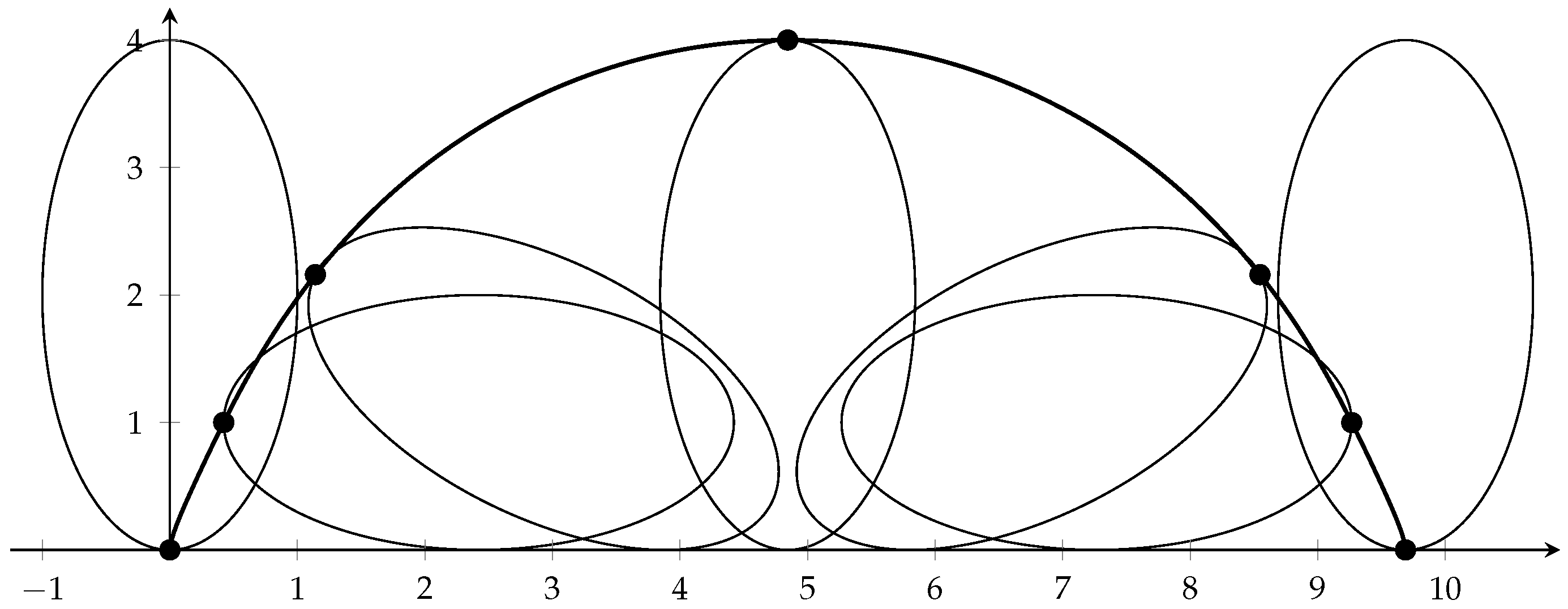What is the area under C and above the x-axis? See Figure 2. Adopting the terminology from the problem, we will refer to such a curve as an elliptic cycloid.

The second author solved this problem, which led us to consider several generalizing questions. First, we considered how arbitrary semi-major/minor lengths affected the area under one arch. More broadly, we wondered how the location of the point on the ellipse chosen to trace the elliptic cycloid affected the shape of the resulting cycloidal curve and the area under one arch. The fact that these two attributes depend on the chosen point is due to the lack of rotational symmetry in the inducing ellipse. In what follows, we will consider a general ellipse rolling along the x-axis and an arbitrary point P on the ellipse; we will then compute the area enclosed by one arch of the resulting elliptic cycloid and the x-axis. To do this, we will use parametric equations to describe the shape of the elliptic cycloid. In addition, we investigate the arc length and curvature. We are unsure if these results are widely known, but cannot find them in the current literature with the exception of [17], which we were informed after submitting our manuscript.

As a final comment here, there do not seem to be many applications of elliptic cycloids with the exception of [18], where elliptic cycloids arise as thermodynamic solutions for equilibrium beach profiles.

2. Parametric Equations for an Elliptic Cycloid

Consider an ellipse E in the Euclidean plane and let P be on E. Suppose E is situated so that P is at the origin and the x-axis is tangent to the ellipse at P. Denote by O the center of the ellipse and let b and a be the lengths of the semi-major/minor, respectively. Let V be the nearest vertex on the major axis that is clock-wise around the ellipse from P and let $s=\angle VOP$. 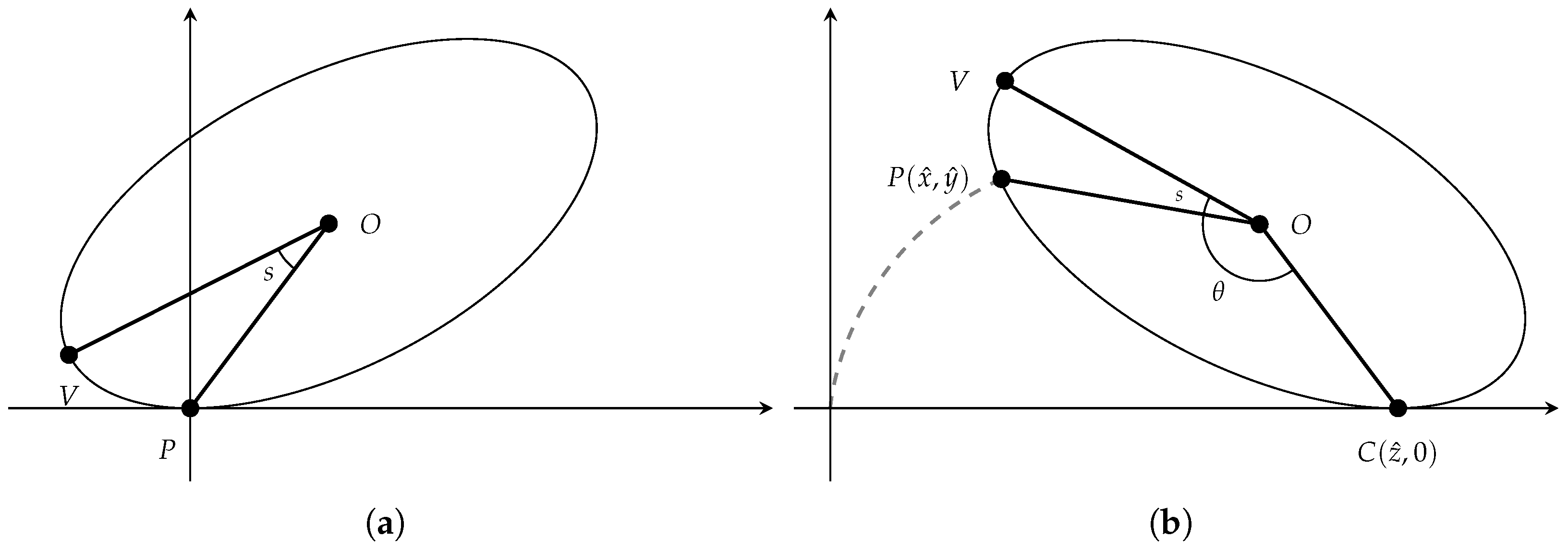If P is chosen to be one of the vertices on the major axis, then take $P=V$ so that $s\in [0,\pi ).$ The left-hand image in Figure 3 shows this initial setup. As the ellipse begins to roll, P traces an elliptic cycloid. We denote the point of tangency to the x-axis by C and define $\theta =\angle POC$. The right-hand image in Figure 3 illustrates this scenario. This section is devoted to finding the coordinate functions giving P as $\theta$ varies from 0 to $2\pi .$

Letting P and C have coordinates $(\widehat{x},\widehat{y})$ and $(\widehat{z},0)$, respectively, we will determine $\widehat{y}$ utilizing the fact that $\widehat{y}$ is the distance between P and the x-axis. We will then compute $|\widehat{z}-\widehat{x}|$ similarly, from which we will be able to determine $\widehat{x}$. To reframe the problem, we utilize the fact that rotations and translations are distance preserving maps. With this, we can compute the desired distances on an oriented ellipse (the adjective will be used to distinguish it from the rolling ellipse). Let $E^{\prime }$ be the ellipse $x^2/a^2+y^2/b^2=1$ with $b>a$. We will use the same identifiers for points on the oriented ellipse so that O is at the origin, V is at $(0,-b)$, P satisfies $\angle VOP=s$, and C is on $E^{\prime }$ with $\angle POC=\theta$. 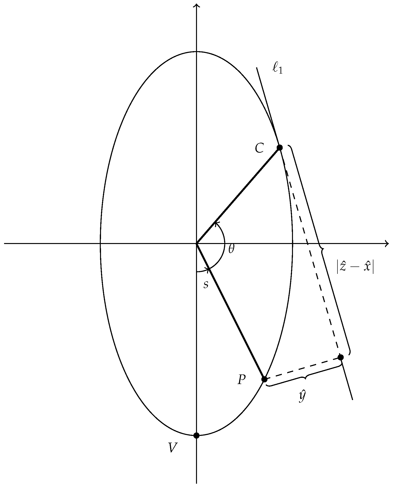Figure 4 provides a visual.

The oriented ellipse $E^{\prime }$ can be represented by the equations

$$x(t)=asin(t),y(t)=-bcos(t),0\le t\le 2\pi ,$$

(1)

parametrized to begin and end one complete path around $E^{\prime }$ at V. We also set $c^2=b^2-a^2$, where c is the distance between the center and a focus. Utilizing these equations, P has coordinates $(asin(s),-bcos(s))$ on the oriented ellipse and C has coordinates $(asin(\theta +s),-bcos(\theta +s)).$

To find the length $\widehat{y}$, we let ${\ell }_1$ be the line tangent to the oriented ellipse at C. This corresponds to the x-axis on the rolling ellipse. Then we have $\widehat{y}=d(P,{\ell }_1)$; see Figure 4. From Equation (1), ${\ell }_1$ has slope

$${\left.{\displaystyle \frac{dy}{dx}}\right|}_{t=\theta +s}={\displaystyle \frac{bsin(\theta +s)}{acos(\theta +s)}}$$

and so the equation for ${\ell }_1$ is given by

$$y+bcos(\theta +s)={\displaystyle \frac{bsin(\theta +s)}{acos(\theta +s)}}(x-asin(\theta +s))$$

or, after simplifying,

$$acos(\theta +s)y-bsin(\theta +s)x+ab=0.$$

(2)

Utilizing the formula for the distance between a point $(x_0,y_0)$ and a line $Ay+Bx+D=0$,

$$d={\displaystyle \frac{|A{y}_0+B{x}_0+D|}{\sqrt{A^2+B^2}}},$$

(3)

Equation (2) and the fact that P has coordinates $(asin(s),-bcos(s))$ on the oriented ellipse gives

$$\widehat{y}=d(P,{\ell }_1)={\displaystyle \frac{ab\left(1-cos(\theta +s)cos(s)-sin(\theta +s)sin(s)\right)}{\sqrt{a^2{cos}^2(\theta +s)+b^2{sin}^2(\theta +s)}}};$$

note that the absolute value is unnecessary since the numerator is always nonnegative. Setting $t=\theta +s$, we have $s\le t\le s+2\pi$ and the previous equation becomes

$$\widehat{y}=y(t)={\displaystyle \frac{ab\left(1-cos(t)cos(s)-sin(t)sin(s)\right)}{\sqrt{a^2+c^2{sin}^2(t)}}}.$$

(4)

We have written the expression in the denominator in terms of a and c rather than a and b only as a matter of convenience.

To find $\widehat{x}$, we first find $\widehat{z}$. Since C is the point $(\widehat{z},0)$ on the rolling ellipse, the arc length function guarantees

$$\widehat{z}={\int }_s^{\theta +s}\sqrt{a^2{cos}^2(r)+b^2{sin}^2(r)}dr={\int }_s^t\sqrt{a^2+c^2{sin}^2(r)}dr.$$

Next, let ${\ell }_2$ be the line through P perpendicular to ${\ell }_1$; in Figure 4, we have only shown the segment of ${\ell }_2$ connecting P and ${\ell }_1$. Knowing the slope of ${\ell }_1$, the equation for ${\ell }_2$ is given by

$$y+bcos(s)={\displaystyle \frac{-acos(\theta +s)}{bsin(\theta +s)}}(x-asin(s))$$

and simplifies to

$$bsin(\theta +s)y+acos(\theta +s)x+b^{2}sin(\theta +s)sin(s)-a^{2}cos(\theta +s)cos(s)=0.$$

Noting $|\widehat{z}-\widehat{x}| =d(C,{\ell }_2)$ and recalling C has coordinates $(asin(\theta +s),-bcos(\theta +s))$ on the oriented ellipse, Equation (3) and some simplification shows

$$\begin{array}{cc}\hfill |\widehat{z}-\widehat{x}|& ={\displaystyle \frac{|b^{2}sin(\theta +s)cos(s)-a^{2}cos(\theta +s)sin(s)-c^{2}cos(\theta +s)sin(\theta +s)|}{\sqrt{a^2{cos}^2(\theta +s)+b^2{sin}^2(\theta +s)}}}\hfill \\ & ={\displaystyle \frac{|b^{2}sin(t)cos(s)-a^{2}cos(t)sin(s)-c^{2}cos(t)sin(t)|}{\sqrt{a^2+c^2{sin}^2(t)}}}.\hfill \end{array}$$

For $\widehat{x}$, the sign of $\widehat{z}-\widehat{x}$ is relevant and from the quantities for $\widehat{z}$ and $|\widehat{z}-\widehat{x}|$, we have

$$\widehat{x}=x(t)={\int }_s^t\sqrt{a^2+c^2{sin}^2(r)}dr-{\displaystyle \frac{b^{2}sin(t)cos(s)-a^{2}cos(t)sin(s)-c^{2}cos(t)sin(t)}{\sqrt{a^2+c^2{sin}^2(t)}}}.$$

(5)

Thus, from Equations (4) and (5), the parametric equations for the elliptic cycloid are given by

$$\widehat{x}=x(t),\widehat{y}=y(t),s\le t\le s+2\pi .$$

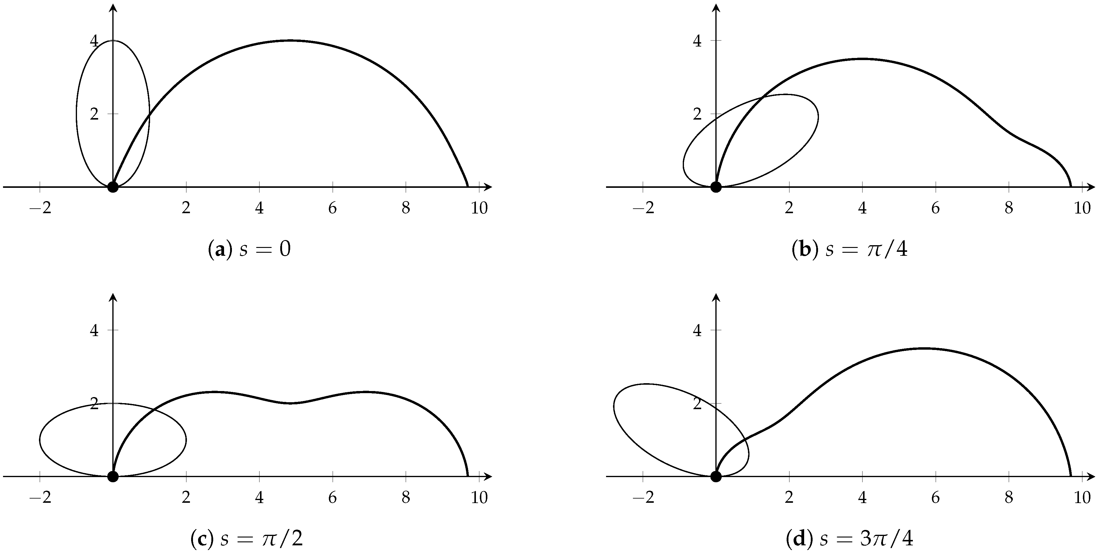
Figure 5 shows one arch of the elliptic cycloids resulting from $s=0$, $\pi /4$, $\pi /2$ and $3\pi /4$ with the initial ellipse orientation for each. For a more interactive visualization, see the link https://www.desmos.com/calculator/dhonxxuruw (accessed on 1 February 2026). On a related note, the text [19] provides an exploration, with code in Maple, for rolling an ellipse along a straight line.

3. Area Formula

Theorem 1.

Let E be an ellipse in the plane and let P be on E, oriented so that P is at the origin and the x-axis is tangent to E at P. Let b and a be the semi-major/minor lengths, respectively, and let V be the nearest vertex on the major axis that is clockwise around the ellipse from P. If $s=\angle VOP$, then the area enclosed by the x-axis and one arch of the elliptic cycloid traced by P is

$$A(s,a,b)=\pi \left(b^2(1+{cos}^2(s))+a^2(1+{sin}^2(s))\right).$$

Notice when $a=b=r$, i.e., E is a circle with radius r, this formula reduces to $3\pi r^2$ as expected. Before giving the proof, we have a few lemmas to simplify forthcoming calculations. The first is a result on residues of odd functions and can be found as an exercise in many complex analysis texts.

Lemma 1.

Let $f:\mathbb{C}\to \mathbb{C}$ be an odd function with isolated singularities at $z=\alpha$ and $z=-\alpha$. Then $\mathrm{Res}(f,\alpha )=\mathrm{Res}(f,-\alpha )$.

Proof. 

For f as given, there exist $R_1,R_2>0$ such that f is analytic on the punctured discs $\{z:0<|z-\alpha |<R_1\}$ and $\{z:0<|z+\alpha |<R_2\}$. Choose $r>0$ with $r<min\{R_1,R_2\}$ and define a curve $\gamma$ by $\gamma (t)=\alpha +r{e}^{2\pi it}$ for $0\le t\le 1$. Then

$$\mathrm{Res}(f,\alpha )={\displaystyle \frac{1}{2\pi i}}{\int }_{\gamma }f(z)dz={\displaystyle \frac{1}{2\pi i}}{\int }_0^{1}f(\gamma (t)){\gamma }^{\prime }(t)dt.$$

Next, define $\delta$ by $\delta (t)=-\gamma (t)=-\alpha -r{e}^{2\pi it}$. Note that $\delta$ is a circle centered at $-\alpha$ with positive orientation. Applying the hypothesis that f is odd yields

$$\begin{array}{cc}\hfill \mathrm{Res}(f,-\alpha )={\displaystyle \frac{1}{2\pi i}}{\int }_{\delta }f(z)dz& ={\displaystyle \frac{1}{2\pi i}}{\int }_0^{1}f(\delta (t)){\delta }^{\prime }(t)dt\hfill \\ & ={\displaystyle \frac{1}{2\pi i}}{\int }_0^{1}f(-\gamma (t))(-{\gamma }^{\prime }(t))dt\hfill \\ & ={\displaystyle \frac{1}{2\pi i}}{\int }_0^{1}f(\gamma (t)){\gamma }^{\prime }(t)dt\hfill \\ & =\mathrm{Res}(f,\alpha ),\hfill \end{array}$$

as desired. □

The second lemma is a simple consequence of the quadratic formula.

Lemma 2.

Let $a,b\in \mathbb{R}$ with $0<a<b$, $c^2=b^2-a^2$, and $\tau =(b^2+a^2)/c^2$. Then $\rho (z)=z^2-2\tau z+1$ factors as $\rho (z)=(z-\alpha )(z-\beta )$, where

$$\alpha ={\displaystyle \frac{{(b-a)}^2}{c^2}}and\beta ={\displaystyle \frac{{(b+a)}^2}{c^2}}.$$

Additionally, $0<\alpha <1<\beta$,

$$\alpha \beta =1,\beta +\alpha ={\displaystyle \frac{2(b^2+a^2)}{c^2}},and\beta -\alpha ={\displaystyle \frac{4ab}{c^2}}.$$

Lastly, we have a lemma for computing integrals of a particular form. The proof is an application of the Residue Theorem. In the statement, $\mathbb{D}$ denotes the open unit disc in the complex plane.

Lemma 3.

Let $a,b\in \mathbb{R}$ with $0<a<b$, $c^2=b^2-a^2$, and $\tau =(b^2+a^2)/c^2$. For α and β as in Lemma 2 and p an even polynomial,

$${\int }_{\partial \mathbb{D}}{\displaystyle \frac{zp(z)}{{(z^4-2\tau z^2+1)}^2}}dz=4\pi i{\displaystyle \frac{\sqrt{\alpha }(\alpha -\beta )p^{\prime }(\sqrt{\alpha })-4\alpha p(\sqrt{\alpha })}{4\alpha {(\alpha -\beta )}^3}}.$$

Proof. 

With the given hypotheses, an application of Lemma 2 shows that $q(z)=z^4-2\tau z^2+1$ has two roots in $\mathbb{D}$ at $z=\sqrt{\alpha }$ and $z=-\sqrt{\alpha }$, and factors as

$$z^4-2\tau z^2+1=(z-\sqrt{\alpha })(z+\sqrt{\alpha })(z^2-\beta ).$$

Letting f be the integrand in the statement of the lemma, we note that f is an odd function by hypothesis and so, by Lemma 1,

$${\int }_{\partial \mathbb{D}}{\displaystyle \frac{zp(z)}{{(z^4-2\tau z^2+1)}^2}}dz=2\pi i\left[\mathrm{Res}(f,\sqrt{\alpha })+\mathrm{Res}(f,-\sqrt{\alpha })\right]=4\pi i\mathrm{Res}(f,\sqrt{\alpha }).$$

Noting that $z=\sqrt{\alpha }$ is a pole of order two for f, we have

$$\begin{array}{cc}\hfill \mathrm{Res}(f,\sqrt{\alpha })& =\underset{z\to \sqrt{\alpha }}{lim}{\displaystyle \frac{d}{dz}}\left[{(z-\sqrt{\alpha })}^2{\displaystyle \frac{zp(z)}{{(z^4-2\tau z^2+1)}^2}}\right]\hfill \\ & =\underset{z\to \sqrt{\alpha }}{lim}{\displaystyle \frac{d}{dz}}\left[{\displaystyle \frac{zp(z)}{{(z+\sqrt{\alpha })}^2{(z^2-\beta )}^2}}\right].\hfill \end{array}$$

Taking the derivative, evaluating the limit, and simplifying gives the conclusion. □

Proof of Theorem 1.

To compute the desired area, we will utilize the parametric area formula

$$A(s,a,b)={\int }_s^{s+2\pi }y(t)x^{\prime }(t)dt.$$

Note that our previous substitution $t=\theta +s$ causes no complications since $dt=d\theta$. From Equation (5), taking the derivative and simplifying yields

$$x^{\prime }(t)={\displaystyle \frac{a^2{b}^2(1-cos(s)cos(t)-sin(s)sin(t))}{{(a^2+c^2{sin}^2(t))}^{3/2}}}.$$

(6)

Then, from Equation (4), we obtain

$$A(s,a,b)=a^3{b}^3{\int }_s^{s+2\pi }{\displaystyle \frac{{(1-cos(s)cos(t)-sin(s)sin(t))}^2}{{(a^2+c^2{sin}^2(t))}^2}}dt.$$

Squaring the expression in the numerator introduces a sum of two summations,

$$1+{cos}^2(s){cos}^2(t)+{sin}^2(s){sin}^2(t)$$

and

$$2cos(s)sin(s)cos(t)sin(t)-2cos(s)cos(t)-2sin(s)sin(t).$$

Considering the first term in the second summation, notice

$${\int }_s^{s+2\pi }{\displaystyle \frac{2cos(s)sin(s)cos(t)sin(t)}{{(a^2+c^2{sin}^2(t))}^2}}dt=0$$

upon substituting $u=sin(t).$ The same conclusion holds for the other two terms and thus

$$A(s,a,b)=a^3{b}^3{\int }_s^{s+2\pi }{\displaystyle \frac{1+{cos}^2(s){cos}^2(t)+{sin}^2(s){sin}^2(t)}{{(a^2+c^2{sin}^2(t))}^2}}dt.$$

(7)

To compute the above integral, we first consider three related integrals. In each case, the change of variables $z=e^{it}$ will be used to convert to an integral around the unit circle. With this change of variables,

$$dt={\displaystyle \frac{dz}{iz}},sin(t)={\displaystyle \frac{1}{2i}}\left(z-{\displaystyle \frac{1}{z}}\right),\mathrm{and}cos(t)={\displaystyle \frac{1}{2}}\left(z-{\displaystyle \frac{1}{z}}\right).$$

Setting $\tau =(b^2+a^2)/c^2$ as in Lemma 2, we have

$$I_1={\int }_s^{s+2\pi }{\displaystyle \frac{1}{{(a^2+c^2{sin}^2(t))}^2}}dt={\displaystyle \frac{-16i}{c^4}}{\int }_{\partial \mathbb{D}}{\displaystyle \frac{z^3}{{(z^4-2\tau z^2+1)}^2}}dz.$$

Applying Lemma 3 with $p(z)=z^2$,

$$I_1={\displaystyle \frac{64\pi }{c^4}}\left({\displaystyle \frac{2\alpha (\alpha -\beta )-4{\alpha }^2}{4\alpha {(\alpha -\beta )}^3}}\right)={\displaystyle \frac{64\pi }{c^4}}\left({\displaystyle \frac{\beta +\alpha }{2{(\beta -\alpha )}^3}}\right)={\displaystyle \frac{\pi (b^2+a^2)}{a^3{b}^3}},$$

where we applied Lemma 2 in the last equality.

Following this same approach,

$$I_2={\int }_s^{s+2\pi }{\displaystyle \frac{{cos}^2(t)}{{(a^2+c^2{sin}^2(t))}^2}}dt={\displaystyle \frac{-4i}{c^4}}{\int }_{\partial \mathbb{D}}{\displaystyle \frac{z(z^4+2z^2+1)}{{(z^4-2\tau z^2+1)}^2}}dt.$$

An application of Lemma 3 with $p(z)=z^4+2z^2+1$ and Lemma 2 yields

$$I_2={\displaystyle \frac{16\pi }{c^4}}\left({\displaystyle \frac{(\alpha -\beta )(\alpha +1)-({\alpha }^2+2\alpha +1)}{{(\alpha -\beta )}^3}}\right)={\displaystyle \frac{16\pi }{c^4}}\left({\displaystyle \frac{\beta +\alpha +\alpha \beta +1}{{(\beta -\alpha )}^3}}\right)={\displaystyle \frac{\pi b^2}{a^3{b}^3}}.$$

For the third integral, we apply the same process with $p(z)=z^4-2z^2+1$ in our application of Lemma 3 to find

$$\begin{array}{cc}\hfill I_3={\int }_s^{s+2\pi }{\displaystyle \frac{{sin}^2(t)}{{(a^2+c^2{sin}^2(t))}^2}}dt& ={\displaystyle \frac{4i}{c^4}}{\int }_{\partial \mathbb{D}}{\displaystyle \frac{z(z^4-2z^2+1)}{{(z^4-2\tau z^2+1)}^2}}dt\hfill \\ & ={\displaystyle \frac{-16\pi }{c^4}}\left({\displaystyle \frac{(\alpha -\beta )(\alpha -1)-({\alpha }^2-2\alpha +1)}{{(\alpha -\beta )}^3}}\right)\hfill \\ & ={\displaystyle \frac{16\pi }{c^4}}\left({\displaystyle \frac{\beta +\alpha -\alpha \beta -1}{{(\beta -\alpha )}^3}}\right)\hfill \\ & ={\displaystyle \frac{\pi a^2}{a^3{b}^3}}\hfill \end{array}$$

To complete the argument, from Equation (7) we obtain

$$A(s,a,b)=a^3{b}^3\left(I_1+{cos}^2(s)I_2+{sin}^2(s)I_3\right)=\pi \left(b^2(1+{cos}^2(s))+a^2(1+{sin}^2(s))\right),$$

completing the proof. □

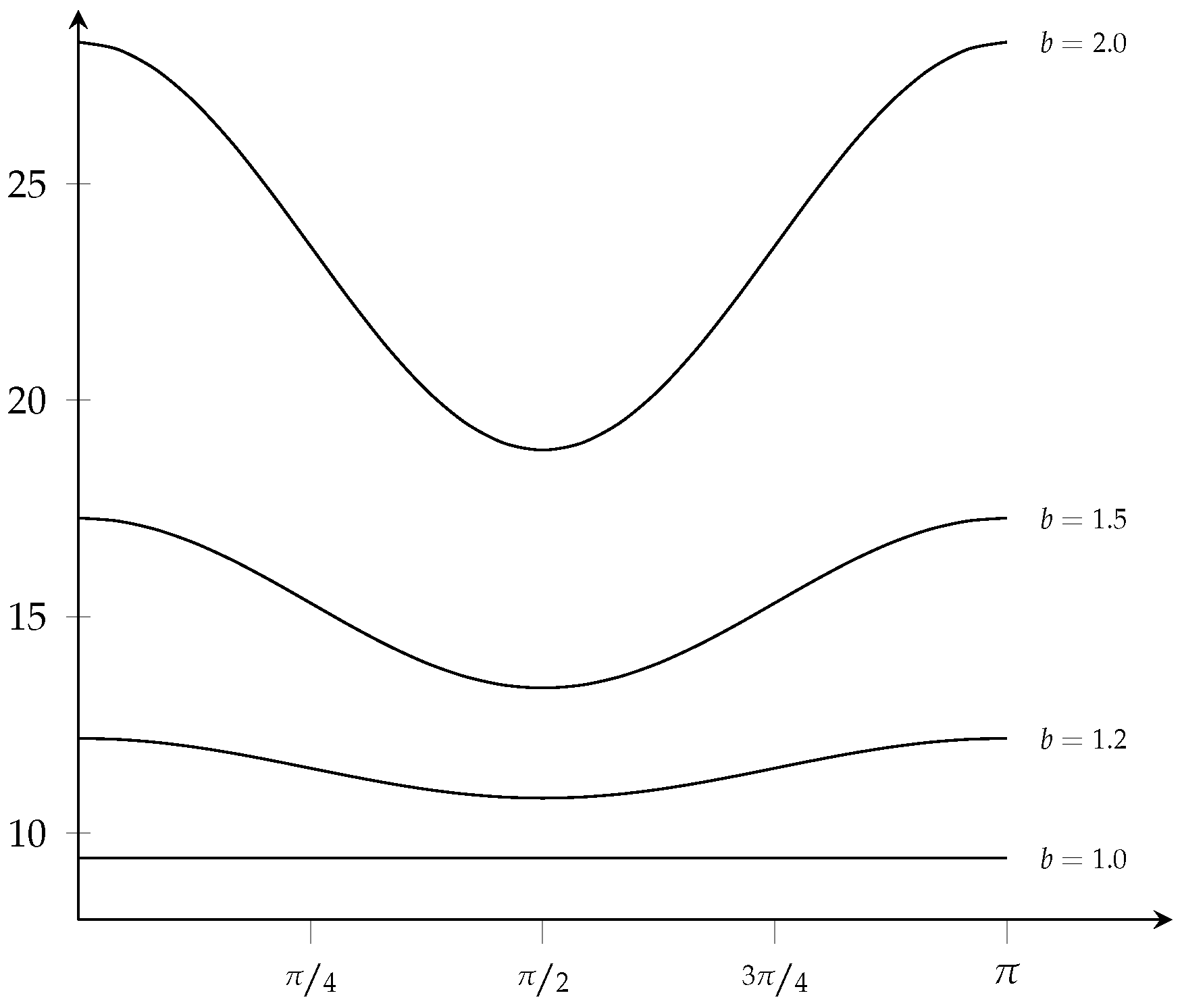
Figure 6 shows the graph of $A(s,1,b)$ for several values of b.

4. Arc Length

Theorem 2.

Let E be an ellipse in the plane and let P be on E, oriented so that P is at the origin and the x-axis is tangent to E at P. Let b and a be the semi-major/minor lengths, respectively, and let V be the nearest vertex on the major axis that is clockwise around the ellipse from P. If $s=\angle VOP$, then the length of one arch of the elliptic cycloid traced by P is

$$L(s,a,b)=ab{\int }_s^{s+2\pi }{\displaystyle \frac{\sqrt{b^2{(cos(s)-cos(t))}^2+a^2{(sin(s)-sin(t))}^2}}{a^2+c^2{sin}^2(t)}}dt.$$

Proof. 

To apply the arc length formula,

$$L(s,a,b)={\int }_s^{s+2\pi }\sqrt{{(x^{\prime }(t))}^2+{(y^{\prime }(t))}^2}dt,$$

we compute $y^{\prime }(t)$ since $x^{\prime }(t)$ is given in Equation (6). After some simplification, we have

$$\begin{array}{cc}\hfill y^{\prime }(t)& ={\displaystyle \frac{ab\left(b^{2}cos(s)sin(t)-a^{2}sin(s)cos(t)-c^{2}cos(t)sin(t)\right)}{{(a^2+c^2{sin}^2(t))}^{3/2}}}\hfill \\ & ={\displaystyle \frac{ab\left(b^{2}sin(t)(cos(s)-cos(t))-a^{2}cos(t)(sin(s)-sin(t))\right)}{{(a^2+c^2{sin}^2(t))}^{3/2}}}.\hfill \end{array}$$

From here, some careful manipulations paired with trigonometric identities gives

$$\begin{array}{cc}\hfill {(x^{\prime }(t))}^2+{(y^{\prime }(t))}^2& ={\displaystyle \frac{a^2{b}^2\left(b^2{(cos(s)-cos(t))}^2+a^2{(sin(s)-sin(t))}^2\right)\left(a^2{cos}^2(t)+b^2{sin}^2(t)\right)}{{(a^2+c^2{sin}^2(t))}^3}}\hfill \\ & ={\displaystyle \frac{a^2{b}^2\left(b^2{(cos(s)-cos(t))}^2+a^2{(sin(s)-sin(t))}^2\right)}{{(a^2+c^2{sin}^2(t))}^2}}.\hfill \end{array}$$

The conclusion now follows. □

First note when $a=b=r$, this formula returns $8r$, as expected. In this case, the integral becomes

$$\begin{array}{cc}\hfill L(s,r)& =r{\int }_s^{s+2\pi }\sqrt{{(cos(s)-cos(t))}^2+{(sin(s)-sin(t))}^2}dt\hfill \\ & =r{\int }_s^{s+2\pi }\sqrt{2(1-cos(t-s))}dt.\hfill \end{array}$$

Substituting $u=t-s$, applying the half-angle trigonometric identity, and integrating completes the calculation,

$$L(s,r)=r{\int }_0^{2\pi }\sqrt{4{sin}^2(u/2)}du=2r{\int }_0^{2\pi }|sin(u/2)|du=2r{\int }_0^{2\pi }sin(u/2)du=8r.$$

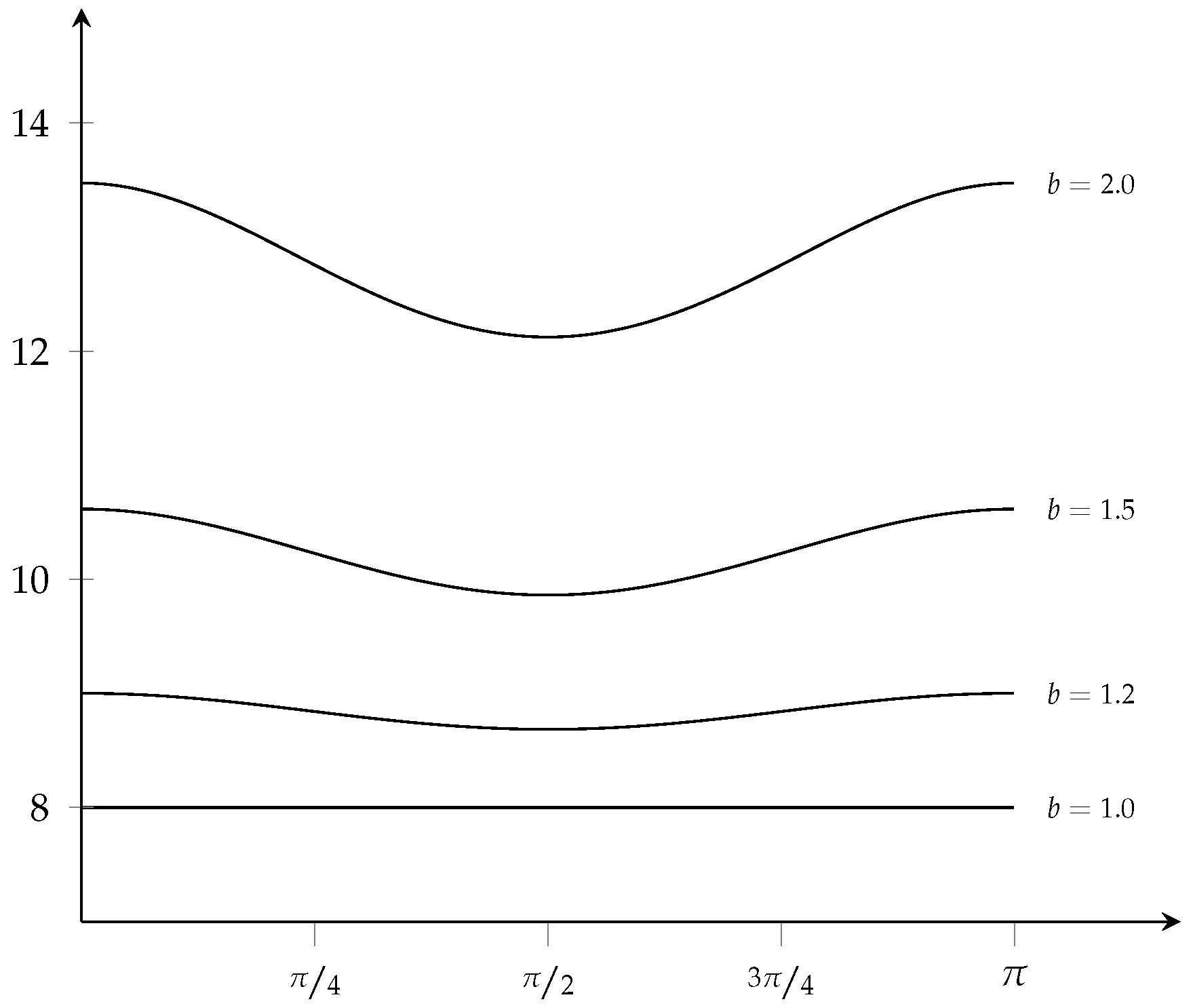
Figure 7 shows the graph of $L(s,1,b)$ for several values of b using numerical approximations. The integral in Theorem 2 is complicated by the radical, but it is not necessarily an elliptic integral. To see this, consider the special case $s=0$, $a=1$, and $b=2.$ The substitution $u=tan(t/2)$ and simplification yields

$$\begin{array}{cc}\hfill {\int }_0^{2\pi }{\displaystyle \frac{\sqrt{4{(1-cos(t))}^2+{sin}^2(t)}}{1+3{sin}^2(t)}}dt& ={\int }_0^{2\pi }{\displaystyle \frac{\sqrt{5-8cos(t)+3{cos}^2(t)}}{4-3{cos}^2(t)}}dt\hfill \\ & ={\int }_0^{\infty }{\displaystyle \frac{8u\sqrt{4u^2+1}}{u^4+14u^2+1}}du.\hfill \end{array}$$

From here, we substitute $v^2=4u^2+1$ and the integral becomes

$$\begin{array}{cc}\hfill {\int }_0^{2\pi }{\displaystyle \frac{\sqrt{4{(1-cos(t))}^2+{sin}^2(t)}}{1+3{sin}^2(t)}}dt& ={\int }_1^{\infty }{\displaystyle \frac{32v^2}{v^4+54v^2-39}}dv\hfill \\ & ={\int }_1^{\infty }{\displaystyle \frac{16-9\sqrt{3}}{v^2-16\sqrt{3}+27}}dv+{\int }_1^{\infty }{\displaystyle \frac{16+9\sqrt{3}}{v^2+16\sqrt{3}+27}}dt,\hfill \end{array}$$

which can be solved using elementary functions. In fact, if $s=0$ and a and b are arbitrary real numbers with $0<a<b$, then the integral in Theorem 2 is solvable with a similar technique. Currently, it is unclear if the integral in question is always solvable using elementary functions or if there are values of s, b and a for which the integral is not solvable using elementary functions and we leave this as an open problem to explore.

5. Curvature

In the statement below, we abbreviate $c_s=cos(s)$ and $s_s=sin(s)$ for convenience.

Theorem 3.

Let E be an ellipse in the plane and let P be on E, oriented so that P is at the origin and the x-axis is tangent to E at P. Let b and a be the semi-major/minor lengths, respectively, and let V be the nearest vertex on the major axis that is clockwise around the ellipse from P. If $s=\angle VOP$, then the curvature $\kappa (\theta )$ of the elliptic cycloid traced by P is

$${\displaystyle \frac{\left|c^2(c_s{cos}^3(t)-s_s{sin}^3(t)-{cos}^2(t)+{sin}^2(t))+b^2{c}_s(cos(t)-c_s)+a^2{s}_s(sin(t)-s_s)\right|}{(b^2{(c_s-cos(t))}^2+a^2{(s_s-sin(t))}^2{)}^{3/2}}},$$

where $c^2=b^2-a^2$, $t=s+\theta$, and $0\le \theta \le 2\pi$.

Proof. 

To compute the curvature, from Equations (4) and (5), we represent the elliptic cycloid by the planar curve $\mathbf{r}(t)=(x(t),y(t))$, where $t=s+\theta$ for $0\le \theta \le 2\pi .$ If we consider the curve in ${\mathbb{R}}^3$, $\mathbf{r}(t)=(x(t),y(t),0)$ and we have

$$\kappa (\theta )={\displaystyle \frac{\parallel {\mathbf{r}}^{\prime }(t)\times {\mathbf{r}}^{″}(t)\parallel }{\parallel {\mathbf{r}}^{\prime }{(t)\parallel }^3}};$$

we will use t as our independent variable and this causes no complications since $dt/d\theta =1$. Simplifying the equation above, we arrive at

$$\kappa (\theta )={\displaystyle \frac{|x^{\prime }(t)y^{″}(t)-x^{″}(t)y^{\prime }(t)|}{({(x^{\prime }(t))}^2+{(y^{\prime }(t))}^2{)}^{3/2}}}.$$

From the proof of Theorem 2, the denominator reduces to

$$({(x^{\prime }(t))}^2+{(y^{\prime }(t))}^2{)}^{3/2}={\displaystyle \frac{a^3{b}^3(b^2{(c_s-cos(t))}^2+a^2{(s_s-sin(t))}^2{)}^{3/2}}{{(a^2{cos}^2(t)+b^2{sin}^2(t))}^3}}.$$

(8)

To compute the numerator, recall our expressions for $x^{\prime }$ and $y^{\prime }$,

$$x^{\prime }(t)={\displaystyle \frac{a^2{b}^2(1-c_{s}cos(t)-s_{s}sin(t))}{{(a^2{cos}^2(t)+b^2{sin}^2(t))}^{3/2}}}$$

and

$$y^{\prime }(t)={\displaystyle \frac{ab\left(b^2{c}_{s}sin(t)-a^2{s}_{s}cos(t)-c^{2}cos(t)sin(t)\right)}{{(a^2{cos}^2(t)+b^2{sin}^2(t))}^{3/2}}}.$$

For simplicity in referencing, set $x_1(t)=1-c_{s}cos(t)-s_{s}sin(t)$ and $y_1(t)=b^2{c}_{s}sin(t)-a^2{s}_{s}cos(t)-c^{2}cos(t)sin(t)$. Taking second derivatives, we have

$$x^{″}(t)={\displaystyle \frac{a^2{b}^2{x}_2(t)}{{(a^2{cos}^2(t)+b^2{sin}^2(t))}^{5/2}}}\mathrm{and}{y}^{″}(t)={\displaystyle \frac{ab{y}_2(t)}{{(a^2{cos}^2(t)+b^2{sin}^2(t))}^{5/2}}},$$

where

$$\begin{array}{cc}\hfill x_2(t)& =b^2{c}_{s}sin(t)-a^2{s}_{s}cos(t)-3c^{2}cos(t)sin(t)+2c^2{c}_s{cos}^2(t)sin(t)\hfill \\ & +2c^2{s}_{s}cos(t){sin}^2(t)\hfill \end{array}$$

and

$$\begin{array}{cc}\hfill y_2(t)& =a^2{b}^2{c}_s{cos}^3(t)+a^2{b}^2{s}_s{sin}^3(t)+b^2(3a^2-2b^2)c_{s}cos(t){sin}^2(t)\hfill \\ & +a^2(3b^2-2a^2)s_s{cos}^2(t)sin(t)-a^2(b^2-a^2){cos}^4(t)+b^2(b^2-a^2){sin}^4(t)\hfill \\ & +2{(b^2-a^2)}^2{cos}^2(t){sin}^2(t).\hfill \end{array}$$

Our numerator now reduces to

$$|x^{\prime }(t)y^{″}(t)-x^{″}(t)y^{\prime }(t)|={\displaystyle \frac{a^3{b}^3|x_1(t)y_2(t)-x_2(t)y_1(t)|}{{(a^2{cos}^2(t)+b^2{sin}^2(t))}^4}}$$

(9)

To complete the proof, a series of trigonometric identities and careful bookkeeping shows $x_1(t)y_2(t)-x_2(t)y_1(t)$ can be written as a product of $a^2{cos}^2(t)+b^2{sin}^2(t)$ and

$$c^2(c_s{cos}^3(t)-s_s{sin}^3(t)-{cos}^2(t)+{sin}^2(t))+b^2{c}_s(cos(t)-c_s)+a^2{s}_s(sin(t)-s_s).$$

If we denote this last expression as $P(t)$, Equation (9) becomes

$$|x^{\prime }(t)y^{″}(t)-x^{″}(t)y^{\prime }(t)|={\displaystyle \frac{a^3{b}^3|P(t)|}{{(a^2{cos}^2(t)+b^2{sin}^2(t))}^3}}.$$

Combining this with Equation (8) yields

$$\kappa (\theta )={\displaystyle \frac{|P(t)|}{(b^2{(c_s-cos(t))}^2+a^2{(s_s-sin(t))}^2{)}^{3/2}}}$$

as desired. □

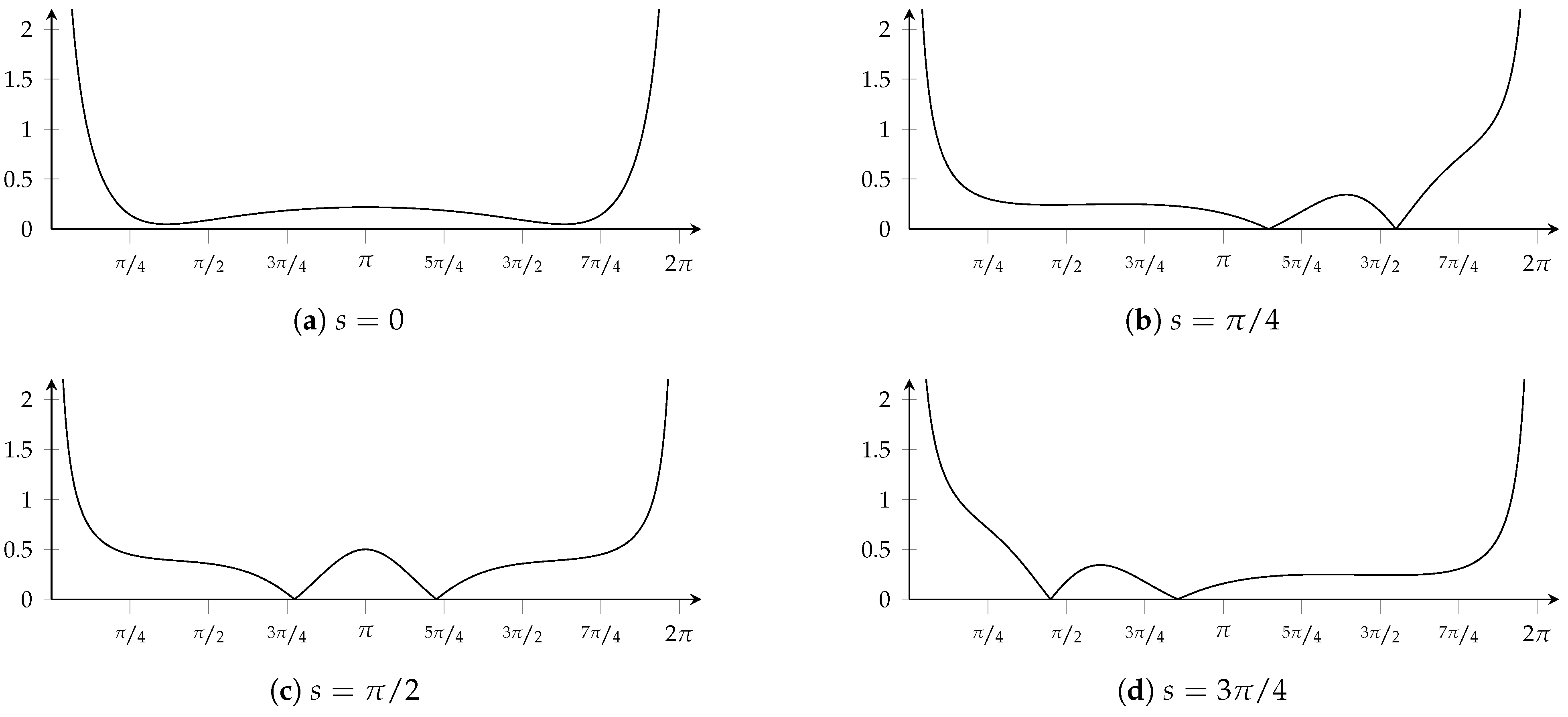
Figure 8 shows curvature plots for $s=0$, $\pi /4$, $\pi /2$, and $3\pi /4$ with $a=1$ and $b=2$. When plotting, we use $\theta$ as the independent variable so that the four graphs have $[0,2\pi ]$ as their common domain. When $a=b=r$, we obtain the curvature of a circular cycloid which is known to be

$$\kappa (\theta )={\displaystyle \frac{1}{4r\left|sin\left(\frac{\theta }{2}\right)\right|}}$$

Unlike circular cycloids, elliptic cycloids can change concavity, which happens when the curvature is zero (though not necessarily at all such points). In general, locating these points is difficult and would require one to find the zeros of $P(t)$. Considering the case $s=\pi /2,$ $P(t)$ simplifies nicely and the curvature becomes

$$\begin{array}{cc}\hfill \kappa (\theta & )={\displaystyle \frac{|(b^2-a^2){sin}^3(t)-2(b^2-a^2){sin}^2(t)-a^{2}sin(t)+b^2|}{(b^2{cos}^2(t)+a^2{(1-sin(t))}^2{)}^{3/2}}}\hfill \\ & ={\displaystyle \frac{|((b^2-a^2){sin}^2(t)-(b^2-a^2)sin(t)-b^2)(1-sin(t))|}{(b^2{cos}^2(t)+a^2{(1-sin(t))}^2{)}^{3/2}}}.\hfill \end{array}$$

Recalling that $t=\pi /2+\theta$, the expression $1-sin(t)$ is zero for $\theta =0,2\pi$. These values also make the denominator zero and correspond to the vertical asymptotes for the curvature. Thus, the curvature is zero when

$$(b^2-a^2){sin}^2(t)-(b^2-a^2)sin(t)-b^2=0.$$

Applying the quadratic formula, we have

$$sin(t)={\displaystyle \frac{1}{2}}-{\displaystyle \frac{\sqrt{b^2-a^2)(5b^2-a^2)}}{2(b^2-a^2)}};$$

note that we do not need to consider the other root of $f(x)=(b^2-a^2)x^2-(b^2-a^2)x-b^2$ since it is always greater than 1 with our assumptions on b and a. The equation above has a solution if and only if $b^2>2a^2$, in which case, since $t=\pi /2+\theta$, we see that the curvature $\kappa (\theta )$ is zero when

$$\theta =-{\displaystyle \frac{\pi }{2}}+arcsin\left({\displaystyle \frac{1}{2}}-{\displaystyle \frac{\sqrt{b^2-a^2)(5b^2-a^2)}}{2(b^2-a^2)}}\right)$$

and

$$\theta ={\displaystyle \frac{\pi }{2}}-arcsin\left({\displaystyle \frac{1}{2}}-{\displaystyle \frac{\sqrt{b^2-a^2)(5b^2-a^2)}}{2(b^2-a^2)}}\right).$$

When $b^2<2a^2$, the curvature is never zero.

A similar analysis can be carried out for $s=0$. Investigating the points where the curvature is zero for other s values requires further analysis of $P(t)$ and we leave this as an open line of inquiry. To explore this set of ideas visually, see the link https://www.desmos.com/calculator/ulswl7xw7z (accessed on 1 February 2026).