Spatial Dependence in Urban Housing Prices: Evidence from Zagreb

Abstract

Housing markets display geographical linkages that contravene conventional regression assumptions; yet, Central and Eastern European towns are markedly underrepresented in spatial econometric research. This study provides a systematic spatial econometric analysis of Zagreb’s housing market. It looks at both asking sale and rental prices throughout the city’s 17 administrative districts. There are five model specifications used in the analysis: Ordinary Least Squares (OLS), Spatial Lag of X (SLX), Spatial Autoregressive Model (SAR), Spatial Error Model (SEM), and Spatial Durbin Model (SDM). The findings demonstrate significant positive spatial autocorrelation in both markets: Global Moran’s I = 0.29 (p = 0.007) for sales and 0.42 (p < 0.001) for rents. LISA analysis finds important groups of high-priced homes in the center districts and lower-priced homes on the edges. Spatial models significantly surpass OLS: SLX exhibits AIC enhancements of 9.90 (sales) and 20.20 (rentals), but SAR and SEM yield no enhancements, suggesting that local spillover effects from adjacent characteristics prevail over global spatial diffusion or correlated shocks. The higher Moran’s I and AIC gains in rental markets show that there are different spatial processes for different types of tenure. These results address a significant empirical deficiency in post-socialist housing research, illustrate that neglecting spatial dependencies may lead to biased estimates and reduced model performance, and furnish methodologically sound evidence that spatial econometric techniques are essential for accurate modeling for precise urban housing analysis in intermediate-sample scenarios. Policy implications stress the need to use spatial approaches in choices about property value, forecasting, and urban planning.

1. Introduction

There are definite trends in the way urban housing markets are laid out. Rich communities tend to be close to each other, while cheap housing is spread out around the city. These patterns come from important economic processes in cities, such as how easy it is to get to jobs and services, how local amenities affect property values, and how neighborhoods affect each other. These kinds of geographical interdependencies go against the usual assumptions of regression; hence spatial econometric methods are needed. This study shows that not taking spatial dependence into account when looking at house prices leads to models that always perform worse. This has direct effects on real estate appraisal and market assessment.

Even if spatial approaches are used a lot, there are still big gaps in the housing markets of Central and Eastern Europe (CEE). After 1989, extensive privatization led to “super-homeownership” systems that are different from those in Western Europe. After privatization in the 1990s, more than 90% of people in Croatia owned their own homes. This created distinctive spatial patterns that mixed socialist-era planning with market pressures.

Zagreb exemplifies an instance that has not been thoroughly examined. Hedonic research investigates pricing determinants; however, none have methodically assessed spatial autocorrelation or contrasted geographical and non-spatial model specifications. This disparity is important because Zagreb is Croatia’s biggest city and makes up more than 25% of the country’s GDP.

This study provides the systematic intra-urban spatial econometric analysis spatial econometric analysis of Zagreb’s housing market, focusing on two inquiries: Do property values demonstrate spatial autocorrelation across districts? Do spatial models do a lot better than regular OLS specifications?

The analysis tests three hypotheses using Census 2021 socio-demographic data and advertised prices from all 17 districts in Zagreb: (1) housing prices show positive spatial autocorrelation, (2) spatial regression models do much better than OLS specifications, and (3) spatial patterns stay the same in both the rental and sales markets. The aggregation at the district level corresponds with administrative borders utilized for policy formulation and Census data collecting, while effectively reflecting local effects with adequate geographical heterogeneity.

This study adds three things to the body of knowledge. First, it fills a vacuum in the research by being the first spatial econometric study of Zagreb’s housing market. This is essential because there is not a lot of thorough research on urban property markets in Central and Eastern Europe. Second, it helps us understand how housing works after socialism by looking at how different parts of the housing market are connected in a unique institutional setting that combines Western-style market tendencies with post-socialist traits. Third, it shows that important spatial patterns may be found even with small spatial units (n = 17) when the right specifications are used. This gives us methodological ideas for working with data that is hard to get.

The results have effects on how real estate works and how cities make decisions. To avoid systematic bias, property valuation needs to use spatial econometric approaches because of spatial autocorrelation. Spatial dependencies suggest that actions taken in one location have effects on surrounding areas; hence, when evaluating policies, spatial multipliers must be taken into account. The high cost of housing in certain areas makes it harder for people to find affordable homes in the whole metropolitan area.

2. Literature Review

Housing prices exhibit consistent spatial patterns that reflect neighborhood effects and locational interdependencies [1,2]. Spatial autocorrelation, defined as the correlation of a variable with itself across geographic space [3], contradicts the assumptions of independence in Ordinary Least Squares (OLS) analysis, potentially causing biased estimates and incorrect inferences [4]. Despite proven applications in numerous contexts [5,6,7,8], Central and Eastern European markets, particularly former Yugoslav countries, remain understudied. This review establishes the theoretical framework, examines applications in CEE and Western Europe, and identifies the research gap this study addresses.

2.1. Theoretical Foundation

Moran’s spatial autocorrelation coefficient (Moran’s I) measures how places change together on a scale from −1 (dispersion) to +1 (clustering). Positive spatial autocorrelation indicates that expensive properties cluster near other expensive properties [9]. Anselin et al. compare statistical significance to spatial randomness. Anselin’s Local Indicators of Spatial Association (LISA) decompose global autocorrelation into local components, revealing High-High clusters, Low-Low clusters, and spatial outliers [1,9,10].

When there is spatial autocorrelation, standard OLS does not work, so explicit spatial models are needed [11,12,13]. The Spatial Autoregressive Model (SAR) incorporates spatially lagged dependent variables to facilitate direct spatial interaction [10]. The Spatial Error Model (SEM) posits that absent variables induce spatial correlation [11]. The Spatial Durbin Model (SDM) incorporates both dependent and independent variables that exhibit spatial lag [12]. The Spatial Lag of X (SLX) model, in contrast, exclusively incorporates spatially lagged covariates, facilitating computation [13,14]. Recent studies look into coordinate systems and neighborhood dummy variables [15] and property features that are not for sale [16].

Lagrange Multiplier tests help model selection figure out the difference between spatial lag and error processes [1]. Information criteria (AIC, BIC) help compare fit that has been corrected for complexity [13]. Monte Carlo simulations demonstrate that SDM and SDEM exhibit robustness even in cases of improper configuration [17]. LeSage and Pace [18], on the other hand, say that people worry too much about how to set up a spatial weights matrix when the right effect decompositions are used.

2.2. Real Estate Markets in Central and Eastern Europe

In spatial econometric literature, Poland’s housing market has been studied the most in Central and Eastern Europe. Tomal [8] employed GWR-SAR on Cracow rentals, documenting significant spatial autocorrelation and substantial improvements to the model. Cellmer et al. [19] employed spatially weighted regression to analyze 380 Polish counties, revealing that structural and locational factors exerted markedly distinct influences on values across various locations. Olszewski et al. [20] found that Warsaw had a strong positive spatial autocorrelation (Moran’s I = 0.22) and that using spatial methods made predictions much more accurate. Trojanek and Głuszak [21] examined the impact of the Warsaw metro on infrastructure, whereas Źróbek et al. [22] investigated the influence of points of interest in Warsaw, Poznań, and Olsztyn. They found that Moran’s I was between 0.12 and 0.25, which showed that amenity capitalization changes based on how prices are spread out. Hungarian research has given us a lot of useful information about what happened after socialism. Horváth et al. [23] examined pricing at the settlement level throughout Hungary and discovered that prices decreased with increasing distance from Budapest. They also discovered that regional disparities persisted during the socialist period. Horváth and Sik [24] used hedonic regression and neural networks to look at Budapest and found that there was a lot of local variation that was not seen. Hlaváček et al. [25] performed a Czech study employing spatially weighted regression in Ústí nad Labem, revealing spatial variability in environmental disamenity effects that reflect inequitable post-socialist restructuring.

New research extends beyond Poland, Hungary, and the Czech Republic. Bălănică and Stănescu [26] examined Bucharest and discovered that prices were grouped in a way that demonstrates the lasting impact of Soviet-era planning on geography. Špirková et al. [27] studied Bratislava and found that the luxury and cheap segments were grouped in a way that was different from other segments. For example, spillovers happened within segments instead of between them. In a study of eight CEE economies, Égert and Mihaljek [7] found that rising prices in the 2000s were caused by rising GDP, interest rates, and the availability of credit. Prices were mostly in capital cities, which could mean that there were spillover effects. Post-socialist environments exhibit distinctive characteristics that differentiate Central and Eastern Europe from Western European systems, including extensive privatization, homeownership rates exceeding 90%, and underdeveloped rental markets [28,29].

2.3. The State of Housing in Croatia

There is less research on Croatian housing than on housing in Poland and Hungary. Slišković and Tica [30] did a full hedonic analysis of Zagreb and found that prices dropped by 2.8% for every kilometer from the center and that being able to get to places was worth more. But their OLS framework did not look for spatial autocorrelation or compare spatial specifications, so it is still not clear if ordinary regression is a good way to explain how things change in Zagreb over time. Kunovac et al. [31] utilized transaction data from the Croatian National Bank spanning 1997 to 2007 to construct hedonic indices, focusing primarily on temporal variations rather than spatial changes. Vizek et al. [32] employed spatial Durbin panel models to examine the impact of tourism on Croatian cities from 2012 to 2019. They discovered substantial positive spatial spillovers. This was the first time that formal spatial econometrics had been used on Croatian data, but the analysis was at the national level across multiple cities, which is different from looking at one city.

2.4. Western European and Global Benchmarks

Marketplaces in Western Europe have standards for how things should be done. Baumont and Legros [6] (2009) demonstrated that spatial effects persisted in Paris metropolitan housing despite the consideration of numerous neighborhood factors. SEM performed significantly better than OLS. Their research demonstrated genuine spillover processes operating independently of evaluated factors. According to Osland’s [5] study in Norway, using spatial Durbin models instead of OLS improved AIC by 15–20%. It also showed that Moran’s I was about 0.31 and that the choice of spatial weights matrix changed the sizes of the numbers but not the main conclusions. Steier’s [33] (2020) study of Germany found very strong spatial autocorrelation (p = 0.45) in Dortmund. This showed that OLS standard errors greatly underestimated uncertainty. Hochstenbach and Arundel’s [34] study in the UK and the Netherlands found that spatial polarization is getting worse and needs clear spatial techniques.

Theoretical foundations emphasize market segmentation and housing submarkets. Goodman and Thibodeau [35] found that when submarkets were clearly defined, spatial disaggregation made hedonic predictions much more accurate (15–25% R² increases). Tu et al. [36] employed semi-variogram estimation to identify data-driven submarkets. They discovered that this method made predictions 17.5% more accurate. They also learned that spatial autocorrelation can be used for two things: to show that a model is wrong and needs to be fixed, and to help find market structure. Arundel et al. [37] looked at geographical inequality in Spain from 2012 to 2022 and used a method that works well in Southern and Eastern Europe after the crisis.

Research conducted globally indicates that spatial relationships extend beyond institutional contexts. In 2026, Paixão and Seidel da Costa employed SAR for Porto Alegre, Brazil, to demonstrate the impact of geographical dependence on the capitalization of school quality [38]. González and Erba [39] developed hedonic methodologies for Buenos Aires, Montevideo, and São Paulo, demonstrating that while specific neighborhood characteristics may vary, fundamental spatial price formation mechanisms: clustering, spillovers, and accessibility gradients remain consistent. Can’s [40] seminal study demonstrated that the incorporation of spatial autocorrelation enhances efficiency. Simulation results indicated that neglecting spatial dependency results in a 20–40% underestimation of the standard error. Dubin [2] elucidated spatial autocorrelation and transformed spatial methodologies into necessary rectifications rather than mere enhancements.

2.5. Methodological Considerations

When there are not many observations, small sample spatial analysis is worried about how reliable it is. Anselin and Florax [41] employed Monte Carlo simulations to examine the characteristics of small samples. They discovered that Moran’s I test still has good power with n = 20–30, but it is less powerful than with larger samples. When n is greater than 25, LM diagnostic tests keep enough of their features. De Paola’s [42] most recent work made maximum entropy methods for valuing real estate with small datasets. When the right frameworks take into account information restrictions, these methods give reliable estimates even when n = 15–25. This makes us sure that district-level analysis (n = 17) can be done.

It is hard to tell if the prices are right because the asking prices and the transaction prices are different. Lyons [43] demonstrated that listing price indices can effectively track transaction fluctuations when accounting for the duration required to sell a property. The correlations exceeded 0.95 for cross-sectional analysis. Han and Strange [44] performed theoretical and empirical analyses that show asking prices give important information about what sellers expect and how the market is doing. This means that asking prices are valid subjects for analysis. Asking prices are useful for spatial analysis that examines relative patterns among neighborhoods rather than absolute values.

The Modifiable Areal Unit Problem (MAUP) happens when you put different properties together into districts. Fotheringham and Wong [45] demonstrated that MAUP systematically distorts correlations through scale effects and zoning effects. Manganelli et al. [46] examined MAUP concerning the correlation between housing density and price. They advised that researchers utilizing administrative boundaries must be explicit regarding the limitations of their work and should interpret their findings as indicative of spatial patterns at the selected scale. Scraped data from internet listings makes people wonder about quality. Boeing [47] recognized potential biases but concluded that online postings provide substantial insights into spatial patterns when coverage is sufficiently comprehensive, as spatial grouping typically endures sampling bias.

2.6. Post-Socialist Housing Context

From 1989 to 1991, when the government changed, post-socialist housing systems changed a lot. Tsenkova [28] said that mass privatization created “super-homeownership” societies, where more than 90% of people owned their own homes. This is much higher than in Western Europe. This made it harder for the rental market to grow and created unique patterns in space that show how property was divided up during the socialist era and how the market changed after the transition. Bežovan [48] points out that Croatia is different from other countries because it privatized quickly in the 1990s, restitution made ownership more complicated, reconstruction after the war slowed reforms, and bad mortgage markets made homes less affordable. These institutional factors influence the formation of spatial price patterns.

Three decades post-transition, the term “post-socialist” as an analytical category is being scrutinized [49]. Housing scholars generally concur that the distinct institutional legacies of CEE markets render them analytically distinct (Stephens et al., 2015) [29]. The post-socialist framework is effective for Zagreb due to the substantial housing stock constructed during the socialist period (approximately 60% from 1945 to 1990), ongoing restitution processes, and a scarcity of social housing. This leads to unique patterns of affordability that make Zagreb different from both Western European cities and other CEE capitals that have gone through different privatization processes.

2.7. Research Gap

There is a lot of research on spatial econometric methods and more and more examples from the real world, but no one has looked at how well spatial and non-spatial models work for the Zagreb housing market. Slišković and Tica [30] conducted a descriptive hedonic study; however, their OLS framework failed to assess spatial autocorrelation or provide estimates of spatial specifications. Vizek et al. [32] employed spatial methodologies on Croatian multi-city data, focusing on inter-municipal tourism spillovers rather than intra-urban interdependence within Zagreb.

This difference is important because Zagreb is Croatia’s main economic center (25% of the country’s GDP) and a regional hub in the Adriatic-Balkan region. There are still some important questions that need to be answered: Is there a lot of spatial autocorrelation in the prices of homes in Zagreb? What is the best spatial specification (SAR, SEM, SLX, SDM)? How much better are spatial methods than OLS? From a methodological standpoint, Zagreb represents a crucial case for the examination of spatial econometrics utilizing constrained spatial units (n = 17 districts). While property-level analysis would provide greater statistical power, district-level analysis offers advantages for understanding the overall spatial structure, aligns with administrative units relevant to planning, and provides a practical framework for laying the groundwork for potential future expansions. Recent methodological advancements [41,42] confirm that reliable insights can be obtained at this scale.

This paper rectifies a significant empirical gap by presenting the formal spatial econometric analysis of the Zagreb housing market, thereby enhancing the limited CEE urban housing literature and offering methodological insights into spatial analysis with constrained sample sizes and asking price data. The study finds out whether spatial methods are necessary for analyzing Zagreb housing or if traditional methods are good enough. This is an important step for future research that will use panel data, better geographical resolutions, and transaction price validation.

3. Research Framework

This research applies systematic spatial econometric analysis to Zagreb’s housing market, examining spatial autocorrelation patterns and comparing spatial versus non-spatial model specifications using advertised listing prices and Census 2021 data.

3.1. Research Goal

The goal of this research is to find patterns of spatial autocorrelation in the pricing of homes in Zagreb and assess how well spatial and non-spatial econometric models work. Instead of trying to figure out exactly how much spillover there is, the study focuses on finding out if spatial methods make traditional methods much better at explaining things. The primary objective is descriptive and methodological: to create empirical foundations for spatial housing research in Zagreb by showing that (1) spatial patterns exist, (2) these patterns support spatial econometric methods, and (3) the choice of model is important for accurately describing how housing prices are formed. In CEE urban research, this trade-off between sample size and data quality is already well known. For example, comparable district-level studies use geographical units that are similarly limited [8,50].

3.2. Research Questions

The empirical analysis is directed by three research questions:

RQ1: Is there spatial autocorrelation in the prices of homes in Zagreb?

This basic question checks to see if home prices group together in certain areas instead of spreading out randomly. Spatial autocorrelation shows that expensive neighborhoods are clustered in certain places, which goes against the OLS independence assumptions and means that spatial econometric methods must be used. Question is answered using Global Moran’s I testing (significant positive values: I > 0, p < 0.05) and LISA analysis to find High-High, Low-Low, or spatial outlier characteristics.

RQ2: Do spatial regression models provide a better fit than traditional OLS?

This question asks if clearly modeling spatial dependencies makes explanations stronger, based on evidence of spatial autocorrelation. Using information criteria, several spatial specifications (SLX, SAR, SEM) are compared and tested to the baseline OLS. A significant improvement in AIC (more than 2 units) shows that spatial models do a better job of capturing how prices are formed.

RQ3: Are geographical patterns the same in both the rental and selling markets?

This robustness inquiry asks if spatial dependencies are general characteristics or if they are exclusive to certain segments. By looking at each section independently, it can be seen if spatial autocorrelation and model improvements apply to both. Consistent findings show that spatial effects are essential to the urban organization of Zagreb, while dissimilar patterns reveal that tenure type influences spatial linkages.

3.3. Hypotheses

H1: 

Housing prices show positive spatial autocorrelation (Global Moran’s I > 0, p < 0.05)

According to urban economic theory, spatial clustering happens because of neighborhood externalities, accessibility gradients, and residential sorting [35,36]. Zagreb’s unique city layout, which includes a compact historic center, socialist-era estates on the outskirts, and new suburbs built after the transition, should lead to clear pricing differences, with the most expensive neighborhoods in the center and the least expensive sections on the outskirts.

H2: 

Spatial regression models fit much better than OLS (AIC improvement > 2)

OLS is misspecified if spatial autocorrelation exists, which violates independence requirements and leads to inefficient estimates [30]. Spatial models fix this problem by using spatially lagged variables or error correlation structures. When spatial methods are used instead of traditional ones, empirical housing studies show that things get a lot better. The AIC usually drops by 5 to 20 units [5,6].

H3: 

There are spatial tendencies in both the rental and selling markets

If spatial dependencies are indicative of essential characteristics of Zagreb’s urban framework: patterns of accessibility, distributions of neighborhood quality, and environmental amenities, they ought to be evident throughout housing submarkets. This hypothesis posits substantial geographic autocorrelation (Moran’s I > 0, p < 0.05) in both markets, as well as enhancements in AIC when spatial models supplant OLS. Finding consistent patterns would show that geographical dependencies are universal market features.

3.4. Contribution

This study offers three primary contributions. First, it presents the formal spatial econometric analysis of the Zagreb housing market, addressing a substantial empirical deficiency. Slišković and Tica [30] recorded hedonic pricing connections by OLS; nevertheless, they did not examine spatial autocorrelation or calculate spatial specifications. Vizek et al. [32] utilized spatial methodologies for Croatian cities, concentrating on inter-municipal tourism spillovers rather than intra-urban dependence inside Zagreb.

Second, the study adds to the small amount of research that has been done on CEE urban housing spatial patterns. Most spatial housing research focuses on Western Europe or North America, with Poland being the most common case in Central and Eastern Europe [8,19]. Croatia, especially Zagreb as the country’s primary metropolitan center, has not been researched enough, even though it has certain unique post-socialist legacies.

Third, the work gives us methodological insights into geographical analysis using limited samples and asking price data. The analysis works at the edge of what is possible with spatial econometrics, with n = 17 districts [8,50]. It shows whether useful insights can still be found even with few geographical units while being honest about the limits that need to be addressed in the future with larger samples and transaction price validation.

4. Data and Methods

4.1. Study Area

The research examines Zagreb, the capital and most populous city of Croatia, with a population of approximately 769,000 (Census 2021). Zagreb is the most important housing market in Croatia because it is the country’s political, economic, and cultural center. The study looks at Zagreb’s 17 official city districts as geographical units.

Zagreb’s 17 districts exhibit substantial spatial heterogeneity reflecting distinct development periods and urban forms. The historic center comprises Donji Grad and Gornji Grad-Medvešćak, characterized by pre-socialist architectural heritage and compact urban fabric. Socialist-era development (1945–1990) produced high-density residential estates, predominantly in Novi Zagreb-istok, Novi Zagreb-zapad, and Trešnjevka-sjever, Trešnjevka-jug, featuring standardized apartment blocks and planned neighborhood units. Post-transition suburban expansion (post-1991) occurred primarily in peripheral districts including Sesvete, Podsused-Vrapče, and Stenjevec, characterized by lower-density single-family housing and automobile-dependent development patterns. Some districts exhibit mixed development profiles reflecting layered urban growth across multiple periods (e.g., Maksimir, Dubrava, Črnomerec). This spatial variability in housing stock vintage, density, and morphology generates the heterogeneous market conditions examined in this analysis.

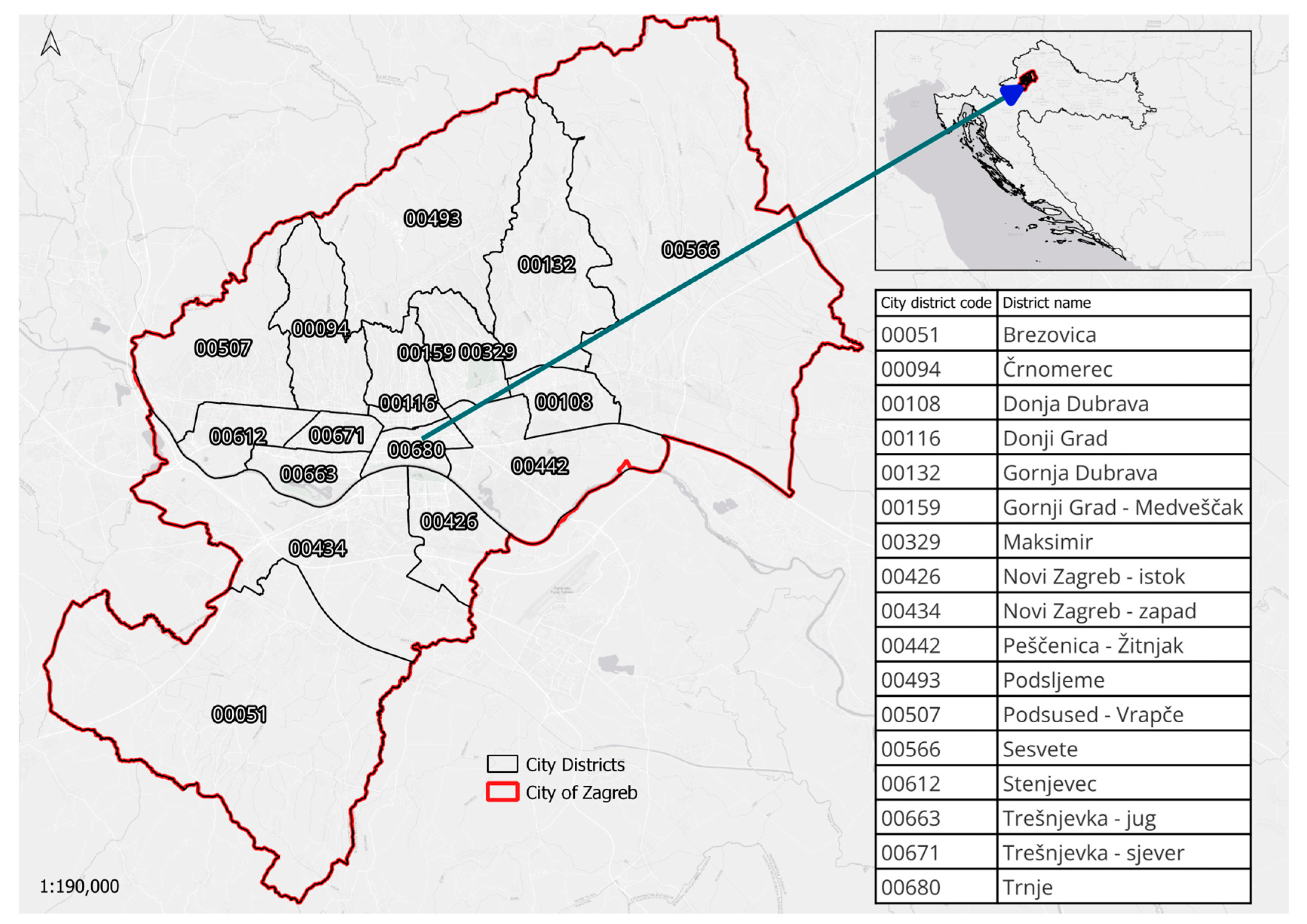
This analysis employs Zagreb’s 17 administrative districts as spatial units. These boundaries were selected for three reasons: (1) Census 2021 demographic data are collected and reported at this administrative level, (2) advertised listing data from the web portal aggregate to district names rather than geocoded addresses due to GDPR restrictions, and (3) administrative districts constitute the official spatial level for municipal governance and policy implementation, making findings directly relevant for urban planning decisions (Figure 1).

It is important to acknowledge that administrative boundaries do not necessarily coincide with housing submarket boundaries. Housing submarkets represent areas where properties serve as substitutes for buyers, often defined by price homogeneity, neighborhood characteristics, and accessibility patterns. Administrative districts, by contrast, reflect political and governance divisions that may cross-cut functional housing market areas. This spatial aggregation represents a data constraint rather than a theoretical choice. Property-level geocoded data would enable data-driven submarket delineation through spatial clustering algorithms (e.g., k-means, SKATER, hierarchical clustering based on price and structural attributes). However, such analysis remains infeasible given current data limitations, where listings identify only district names without specific addresses.

Despite these limitations, district-level analysis remains analytically viable and policy-relevant. This district-level aggregate (n = 17) exemplifies a compromise between geographical resolution and analytical viability. Districts are meaningful administrative units important for urban planning and policy implementation; combining data from different listings reduces noise; and recent methodological work shows that spatial econometric methods still work well even with limited observations. Anselin and Florax used Monte Carlo simulations to look at small sample properties [41]. They found that Moran’s I test still works well with 20 to 30 observations. De Paola [42] devised methodologies tailored for appraising real estate with constrained datasets, demonstrating that meticulous specification can yield precise estimates despite reduced sample size. Results represent spatial patterns at the administrative scale and should not be interpreted as capturing finer-grained within-district heterogeneity. The choice of spatial units may introduce aggregation bias if housing submarkets cross district boundaries; however, the practical trade-off balances statistical power limitations against the fact that using non-spatial methods when spatial grouping is expected and easy to see does not make sense. Future research with geocoded transaction data could refine these findings through data-driven submarket analysis and sensitivity testing of alternative spatial delineations.

4.2. Data Sources

4.2.1. Housing Price Data

Housing price data are derived from online real estate listings scraped from Index oglasi (www.index.hr/oglasi, accessed on 15 July 2025), Croatia’s leading real estate advertising platform, between July 2024 and July 2025. Web scraping techniques were employed to systematically collect listing information across Zagreb’s 17 districts. The raw dataset comprises 9959 sale listings and 4571 rental listings, which were cleaned and filtered to the specified temporal coverage.

The dataset includes all advertised residential apartment listings available on the platform during the collection period, encompassing both existing housing stock and new construction units without systematic differentiation. The platform does not provide a standardized attribute indicating new-build status, preventing reliable classification into existing versus new-build segments. Consequently, the analysis treats all listings as a unified housing market reflecting actual supply composition.

This method is based on what happens in the real world: buyers and renters look at both existing and new-build stock at the same time, and both groups help create the spatial price patterns we see. While new building may have different prices or locations, excluding out these listings would not show the true state of the market or the spatial dependencies that arise from a full housing supply. The district-level aggregation reduces the chance of compositional effects even more because the mean prices include a mix of different housing vintages that show how each district has grown and what kind of homes are currently available.

The housing price data comes from internet real estate listings that show the prices people are asking for their homes between July 2024 and July 2025. Prices in the sale market are shown as price per square meter (EUR/m²), which is how buyers usually figure out the value of a property. In the rental market, prices are shown as total monthly rent (EUR/month), which is how tenants usually think about their monthly cash flow requirements. These differing units make it impossible to directly compare the sizes of coefficients across markets, but they do allow for proper analysis within each market segment and comparison of spatial patterns (autocorrelation, model ranks) across segments.

The use of asking prices instead of transaction pricing is due to a lack of data. The Croatian land registry transaction data are not publicly available at the spatial resolution necessary for district-level analysis. However, recent research shows that listing prices have good correlations (r > 0.95) with transaction prices in cross-sectional spatial analysis. This means that relative spatial patterns are still true even if absolute price levels are different [43,44]. For spatial analysis centered on relative patterns among neighborhoods rather than absolute valuation, asking prices effectively reflect the underlying spatial interdependence.

The data on advertised listings were gathered for academic research purposes only after Index promocija d.o.o. gave their clear written authorization (September 2024). The platform’s Terms of Use allowed for non-commercial use of publicly viewable information while still following GDPR privacy rules.

All of the data that was obtained is publicly available listing information (prices, square meters, number of rooms, year built) that has been combined to show the district level. No personal information, user identities, or individual addresses were gathered or processed, which means that the GDPR rules were fully followed. The study only looks at overall geographical trends across Zagreb’s 17 administrative districts, not at individual properties or users. Typical web scraping methods were used to acquire data from publicly available listing sites. All collected data were anonymized. No data about individuals is kept, exchanged, or used after it has been grouped together for statistical analysis.

Section 2.6 of the platform’s Terms of Use says that you can copy and share listing content for non-commercial reasons as long as you do not post any personal information. This study follows these rules exactly by only looking at combined district-level statistics and not copying individual listings or user information. All analytical code and disaggregated data are kept private and not shared with anyone else, as required by GDPR and the authorization given.

4.2.2. Census Data

The socio-demographic and housing structural data are derived from the 2021 Census executed by Croatia’s State Statistical Office. Four variables are selected following established post-socialist housing literature that identifies these as theoretically relevant determinants of spatial price patterns [23,28,29,36], while also being available at the district level.

Private Ownership Percentage: Croatia’s widespread privatization in the 1990s led to “super-homeownership,” with rates over 90% [28]. Regions with more private ownership respond differently to market signals than regions with social housing or other types of housing [29].

Vacancy Rate: A measure from the supply side that shows when there are too many empty units, which makes prices go down. Spatial clustering creates submarkets [33]. Post-socialist situations have more empty homes because families keep their homes as investments [33].

Housing density is the way that buildings are built in cities. High density means apartment buildings from the time of socialism, while low density means single-family homes in the suburbs after socialism. Infrastructure, the character of the neighborhood, and supply limits [33] are all things that affect supply.

Average household size is a demographic proxy for demand-side. Larger households want bigger homes; this shows what kind of neighborhood it is (families vs. singles/couples). The legacy of socialist housing allocation persists [33].

This simple specification makes it clear that there are only n = 17 degrees of freedom. Adding four covariates stops overfitting [11] while still getting the important supply-demand dynamics. The focus on spatial effects rather than comprehensive prediction substantiates limited controls.

4.2.3. Spatial Data

Digital boundary files are provided for the 17 districts of Zagreb from official government geographic data sources. The spatial weights matrix was made using these files.

4.3. Data Characterization

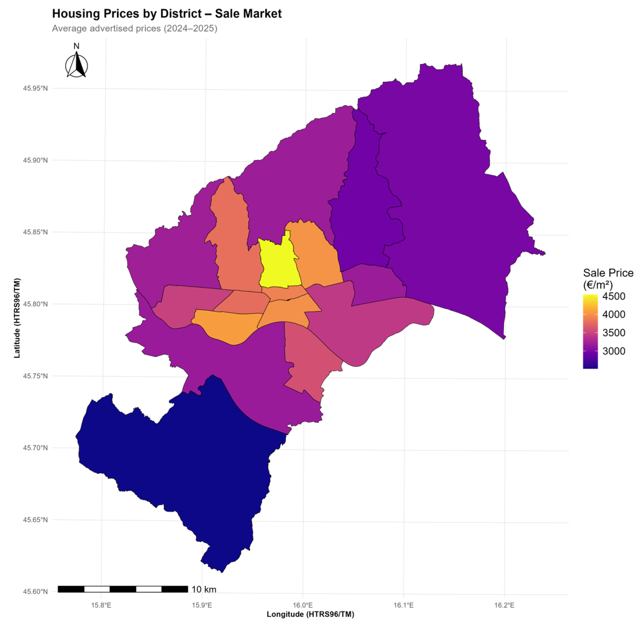
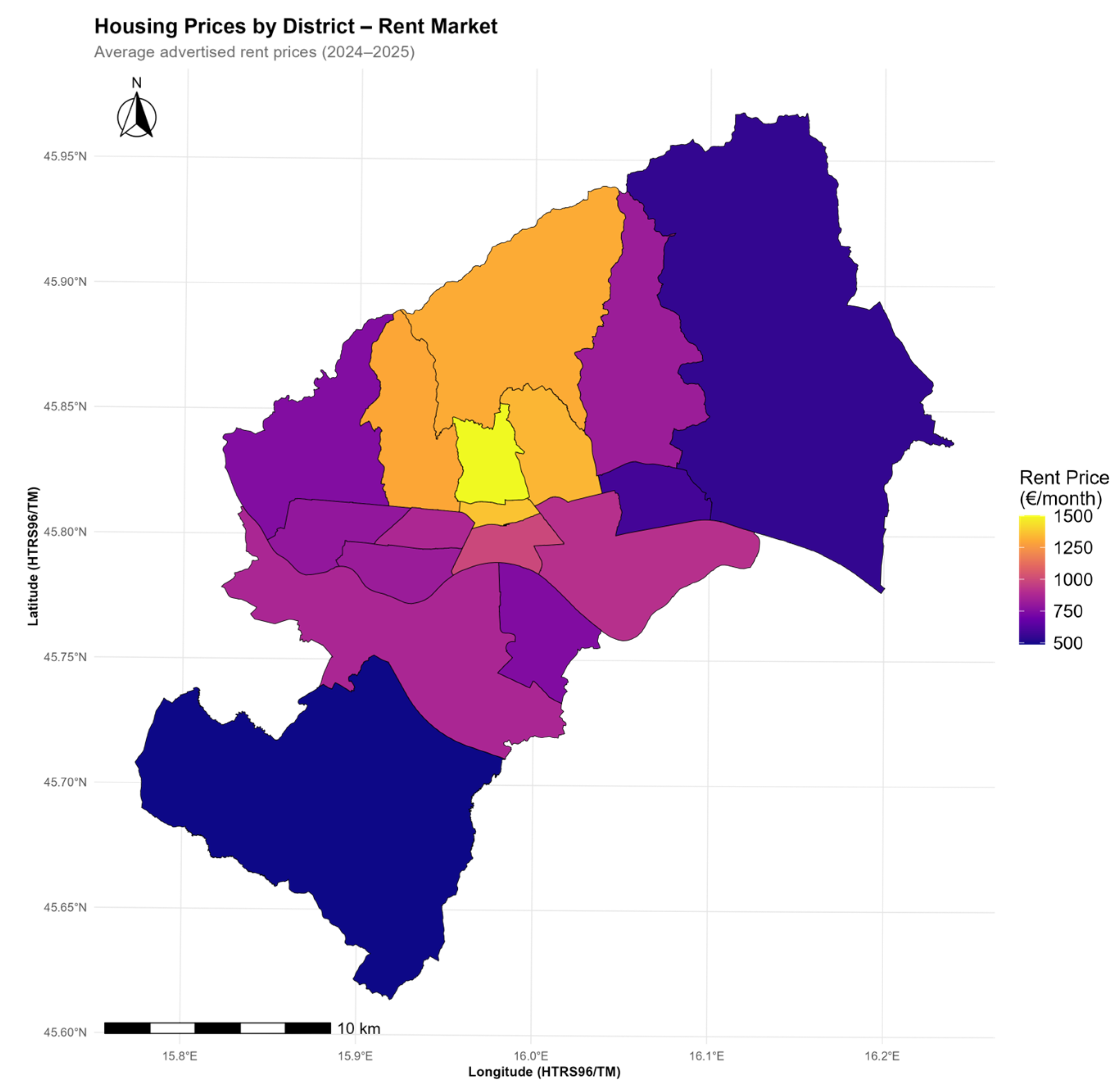
This section presents descriptive statistics and spatial distribution patterns for the housing price datasets.

Table 1. Descriptive statistics.

Variable	Mean	SD	Min	Max
Sale price (EUR/m2)	3517.34	512.42	2611.31	4566.79
Rent price (EUR/month)	942.84	310.56	537.98	1598.15
Private ownership (%)	92.15	3.48	83.21	96.54
Vacancy rate (%)	17.84	2.50	14.23	23.89
Housing density (units/km2)	2847.62	2156.33	438.17	7891.45
Average household size	2.59	0.38	1.96	3.22

summarizes key statistical properties of sale and rental prices across Zagreb’s 17 districts, while Figure 2 and Figure 3 illustrate their spatial distribution.

Dependent variables: (1) Sale: average advertised price (EUR/m²), (2) Rent: average advertised monthly rent (EUR/month). The independent variables are (1) the percentage of private ownership, (2) the percentage of vacant units, (3) the number of units per square kilometer, and (4) the average number of people per household.

Table 1 presents descriptive statistics for housing prices and control variables across Zagreb’s 17 districts, revealing substantial spatial variation in market conditions.

Sale prices average 3517 EUR/m² (SD = 512), with a 75% differential between least and most expensive districts (2611–4567 EUR/m²). Rental prices average 943 EUR/month (SD = 311), exhibiting wider relative dispersion (33% vs. 15% for sales), suggesting stronger spatial differentiation in rental markets.

Control variables demonstrate spatial heterogeneity. Private ownership averages 92.2% (SD = 3.5%), reflecting Croatia’s super-homeownership legacy from mass privatization [28]. Vacancy rates average 17.8% (SD = 2.5%), considerably higher than Western European levels, consistent with post-socialist patterns. Housing density varies dramatically (438–7891 units/km²), reflecting diverse urban forms from dense socialist-era estates to low-density peripheral zones. Average household size ranges from 1.96 to 3.22 persons (mean = 2.59).

Variance Inflation Factors (VIF) were used to check for multicollinearity amongst independent variables. Housing_Density (VIF = 2.08) and Avg_Household_Size (VIF = 2.55) showed good values that were much below normal limits. But Private_Ownership_Pct (VIF = 17.81) and Vacancy_Rate (VIF = 18.69) showed a lot of collinearity, which is because they both come from the same place: post-socialist housing dynamics, where patterns of broad privatization are linked to patterns of vacancy. Sensitivity analysis was applied to see how the results would change if each collinear variable was left out. For the sale market, excluding Private_Ownership while keeping Vacancy_Rate, Housing_Density, and Avg_Household_Size resulted in a statistically equivalent model fit to the original four-variable specification (ΔAIC = −1.98, below the threshold of 2 for substantial difference), while also removing multicollinearity (maximum VIF reduced to 2.55). This three-variable specification is used to analyze the sale price. Excluding either Private_Ownership (ΔAIC = +12.12) or Vacancy_Rate (ΔAIC = +14.78) significantly diminished model fit in the rental market, demonstrating that both variables provide distinct explanatory power despite collinearity. The original four-variable specification is preserved for rental analysis. High VIF makes standard errors bigger, but it does not change the coefficient estimations. Because the study is more about documenting spatial patterns than measuring effects exactly, it is more important to have a wide range of variables than to stick to stringent VIF levels for the rental market. All of the studies that follow use market-specific specifications. For sale prices, there are three covariates (Vacancy_Rate, Housing_Density, and Avg_Household_Size), while for rental prices, there are four (adding Private_Ownership_Pct). Tests for spatial autocorrelation and comparisons of models show that spatial patterns (Global Moran’s I, LISA clusters) and rankings of model performance stay strong across different specifications.

After evaluating multicollinearity, market-specific model specifications were utilized. There are three variables in sale price models (Vacancy_Rate, Housing_Density, and Avg_Household_Size). In rental pricing models, there are four covariates (adding Private_Ownership_Pct). Both markets agree that SLX is the best spatial model because it shows consistent spatial spillover effects across all housing segments.

4.4. Spatial Weights Matrix

A queen contiguity weights matrix formalizes spatial relationships by treating districts that share boundaries or vertices as neighbors. Queen contiguity is broader than rook contiguity because it includes diagonal adjacencies that are important for urban spatial processes. The matrix is set up so that the weights for each district add up to 1.0. This helps you think of spatial lag terms as neighborhood averages. The spdep package in R [51] was utilized for construction, adhering to established methodologies documented in the spatial econometrics literature [1,12].

4.5. Analytical Methods

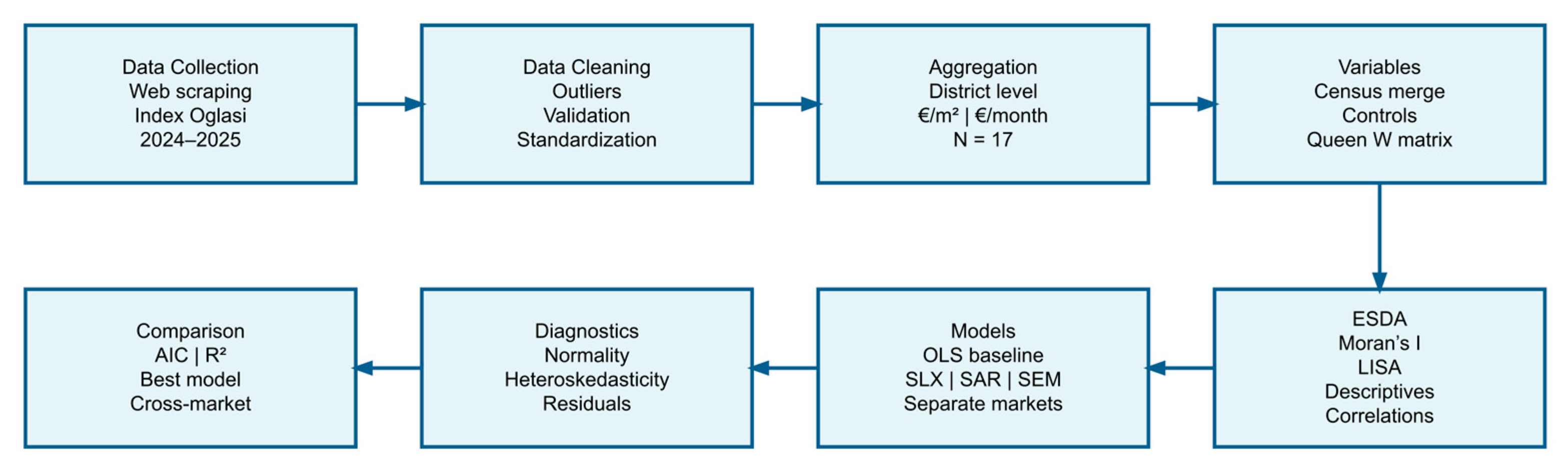
Figure 4 presents the methodological workflow employed in this study. The analysis follows a sequential eight-step process from data collection through model comparison, ensuring systematic evaluation of spatial dependencies in Zagreb’s housing markets.

4.5.1. Exploratory Spatial Data Analysis

The analysis begins with exploratory spatial data analysis to detect and visualize spatial patterns in housing prices. Global Moran’s I quantifies the overall degree of spatial autocorrelation, with values ranging from −1 (perfect dispersion) to +1 (perfect clustering). Under the null hypothesis of spatial randomness, statistical significance is assessed using 999 permutations [1]. Local Moran’s I (LISA) decomposes global autocorrelation into location-specific contributions, identifying four spatial cluster types: High-High clusters (expensive districts with expensive neighbors), Low-Low clusters (affordable districts with affordable neighbors), High-Low outliers (expensive districts surrounded by affordable neighbors), and Low-High outliers (affordable districts surrounded by expensive neighbors). Statistical significance is determined via conditional permutation (p < 0.05). These diagnostics reveal whether spatial autocorrelation stems from isolated outliers or represents systematic citywide patterns.

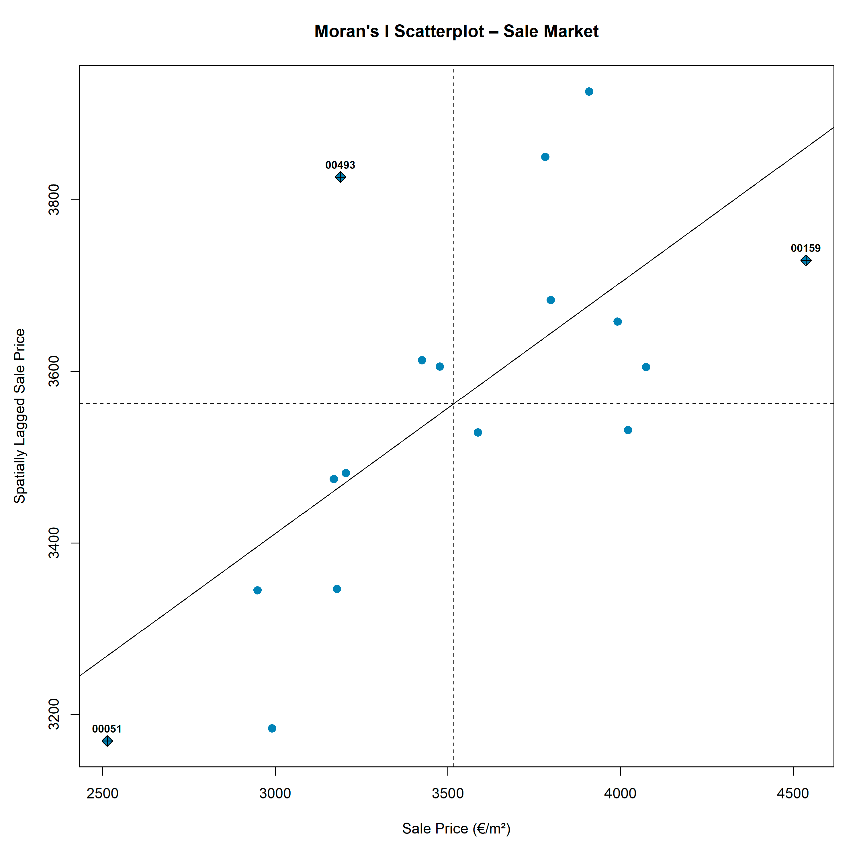
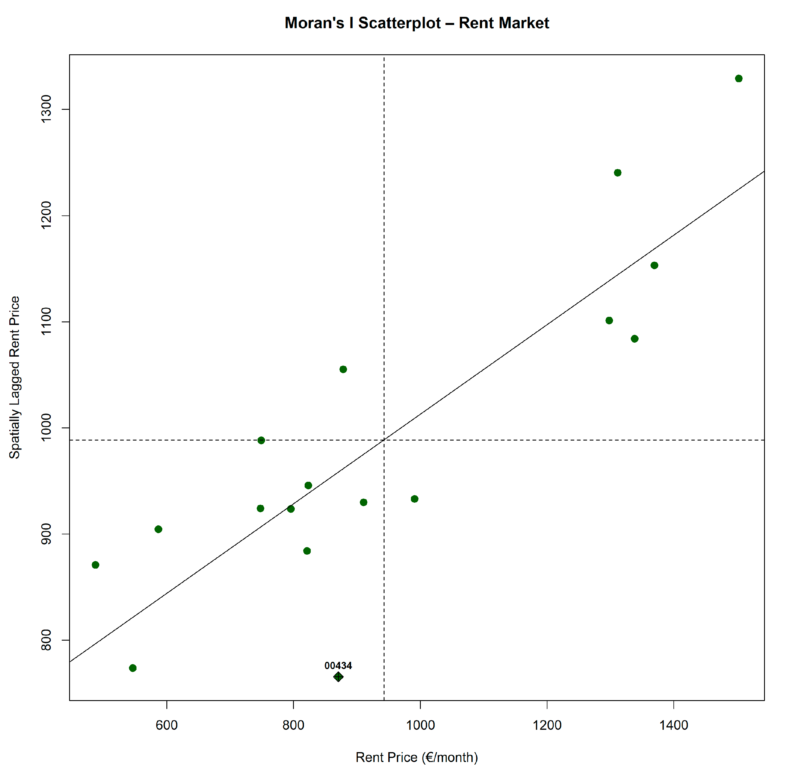
These diagnostics reveal whether spatial autocorrelation stems from isolated outliers or represents systematic citywide patterns. Results are visualized using Moran scatterplots, in which standardized prices are plotted against their spatial lags. The diagonal line represents the OLS fit whose slope equals Moran’s I. Dashed lines indicate variable means, dividing the plot into High-High, Low-Low, High-Low, and Low-High quadrants. Diamond symbols identify districts deviating notably from the spatial trend, labelled by district code.

4.5.2. Spatial Regression Models

Four model specifications are estimated to assess the role of spatial dependencies:

OLS (Baseline): Standard non-spatial hedonic regression serving as the comparison benchmark.

y = Xβ + ε

(1)

Spatial Lag of X (SLX): Incorporates spatially lagged independent variables, capturing local spillover effects from neighboring district characteristics without assuming global spatial dependence [13,14]. This specification allows characteristics of adjacent districts to influence local prices through localized externalities.

y = Xβ + WXθ + ε

(2)

Spatial Autoregressive Model (SAR): Includes a spatially lagged dependent variable, where p represents the spatial autoregressive coefficient measuring direct price spillovers across districts [1]. This specification is appropriate when prices in one district directly influence prices in adjacent districts through market mechanisms such as spatial arbitrage or comparison shopping.

y = pWy + Xβ + ε

(3)

Spatial Error Model (SEM): Models spatial dependence through correlated error structure, where λ denotes the spatial error coefficient capturing effects of unobserved spatially correlated factors [4]. This specification suits contexts where omitted spatially varying characteristics such as school quality, environmental amenities, or infrastructure access, generate correlated residuals.

y = Xβ + u

(4)

u = λWu + ε

(5)

Spatial Durbin Model (SDM): Combines both spatially lagged dependent variable and spatially lagged independent variables, allowing simultaneous estimation of direct price spillovers (p) and indirect effects from neighboring district characteristics (θ coefficients on WX terms) [13]. This specification is appropriate when both direct spatial price interdependence and localized spillover effects from neighboring attributes operate simultaneously. The SDM provides the most flexible spatial specification, nesting both SAR and SLX as special cases, and allows decomposition of total effects into direct (own-district) and indirect (cross-district) components.

y = ρWy + Xβ + WXθ + ε

(6)

The baseline OLS specification functions as a non-spatial benchmark and excludes district-level fixed effects. This design choice is based on the fact that the sample size is limited (n = 17) and the structure is cross-sectional. Adding district dummies would use up degrees of freedom and make perfect multicollinearity. The primary aim of the research is to examine spatial dependence among districts. Adding fixed effects would take care of all the differences between districts, which is what spatial models are meant to do by using neighborhood spillover mechanisms. In spatial econometric comparisons, this method is standard since OLS gives a baseline that is not spatial. Instead, observed covariates and, in spatial models, neighborhood spillover terms (WX, Wy, Wu) are used to show how different districts are from each other.

4.5.3. Model Estimation and Comparison

Ordinary least squares are used to get OLS estimations. Spatial models utilize maximum likelihood estimation with the spatialreg package in R [52]. Separate estimates are made for the sale and rental sectors so that comparisons can be made between different segments.

The Akaike Information Criterion (AIC) and the coefficient of determination (R²) are used to measure how well a model works. AIC differences of more than 2 units signify significant enhancement of the model [53].

4.5.4. Diagnostic Tests

Residual normality is assessed via Shapiro–Wilk tests, while heteroskedasticity is examined using Breusch-Pagan tests. All analyses are conducted in R 4.4.2 using the following packages: sf (spatial data handling), spdep (spatial weights and autocorrelation), spatialreg (spatial regression), and ggplot2 (visualization).

5. Results

This section presents empirical findings addressing the three research questions: spatial autocorrelation patterns (RQ1), spatial versus non-spatial model performance (RQ2), and pattern consistency across market segments (RQ3).

5.1. Spatial Autocorrelation Analysis

5.1.1. Sale Market Spatial Patterns

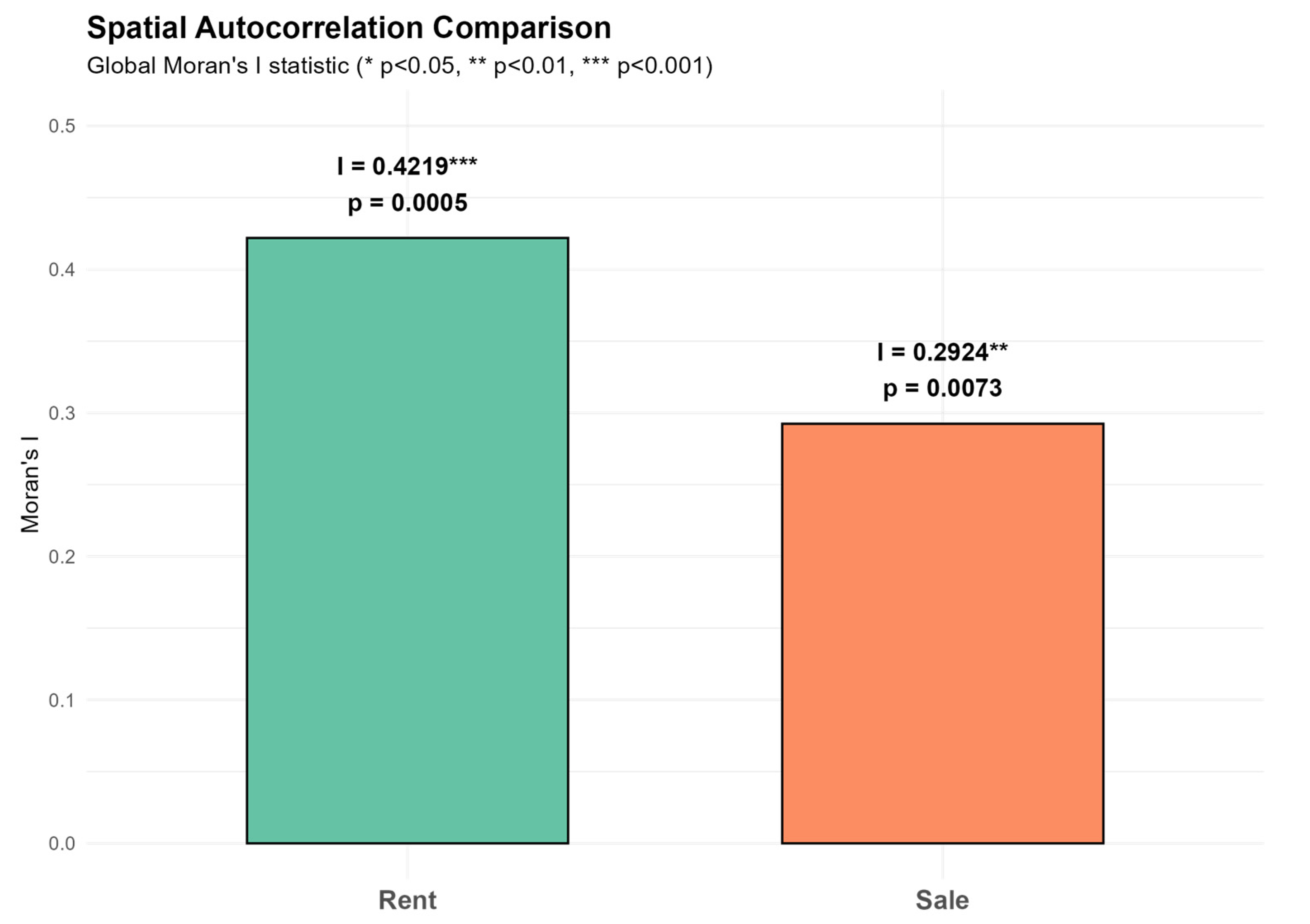
The Global Moran’s I for sale prices is 0.2924 (p = 0.0073), which is strong evidence of positive spatial autocorrelation that is very different from spatial randomness. This supports Hypothesis 1. This intermediate number shows that expensive districts are grouped together in space. The magnitude (I = 0.29) shows that the clustering is moderate. It is not as strong as in certain Western European cities [6], but it is still significant because Zagreb is tiny and the district-level resolution is low. A higher spatial resolution would probably show larger clustering, since aggregation usually makes spatial autocorrelation measures less accurate [45]. Figure 5 shows the Moran scatterplot. Most of the points are in the High-High and Low-Low quadrants, which means that the sale market has positive spatial autocorrelation.

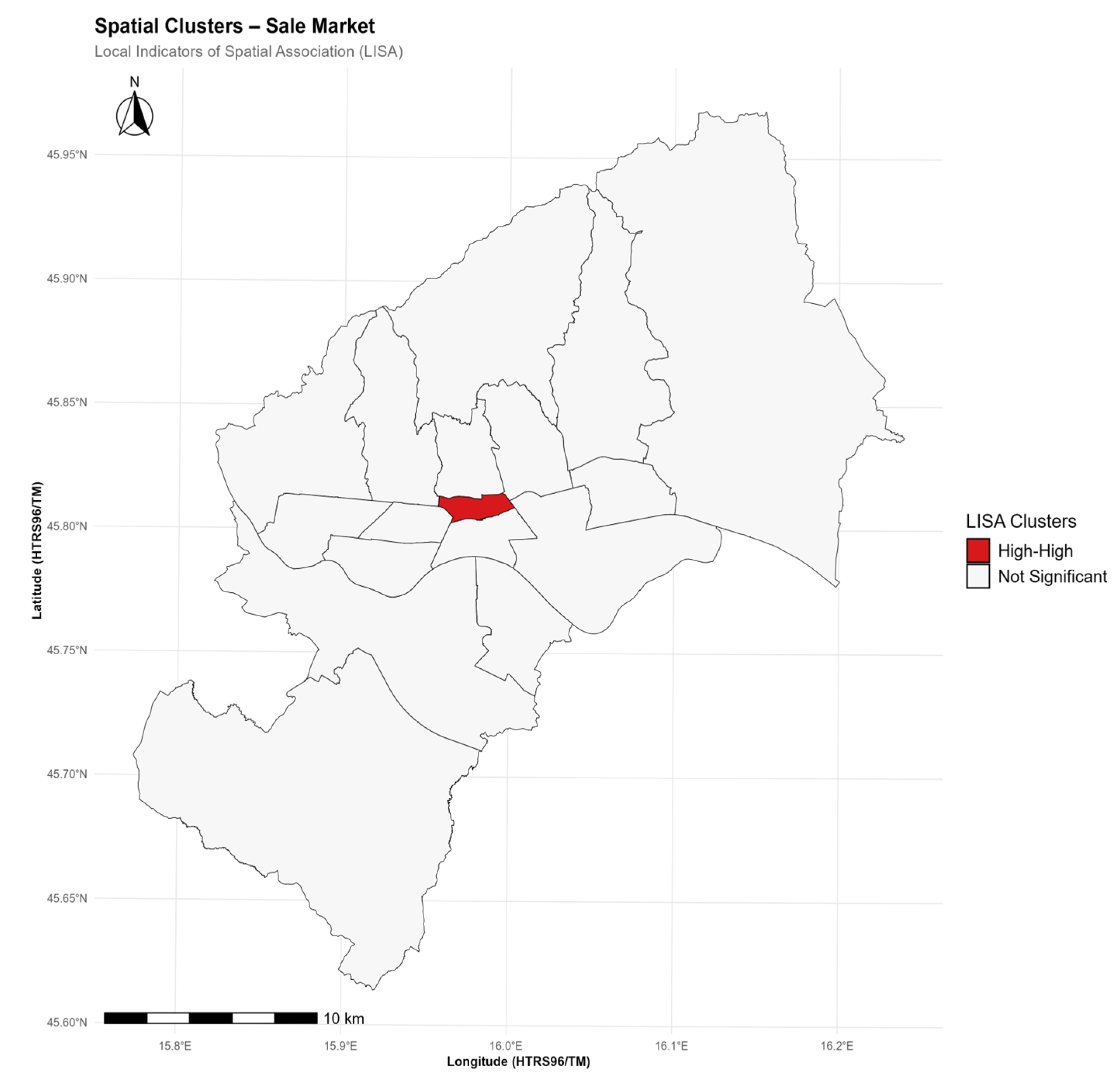
LISA analysis shows one big cluster: Donji Grad is High-High (p < 0.05) because it has a high sale price of 3909 EUR/m² and is surrounded by neighbors who are also pricey. The high price of this ancient city core is due to the high concentration of cultural attractions, architectural legacy, and easy access, which all have favorable effects on the surrounding area. No major Low-Low clusters appear, indicating that cheap housing does not aggregate in physically contiguous peripheral zones at the district level. Figure 6 shows important clusters and how prices are spread.

5.1.2. Rent Market Spatial Patterns

The Global Moran’s I for rental prices is 0.4219 (p = 0.0005), which means that there is more geographical autocorrelation than in the selling market. This higher value shows that rental housing has more pronounced geographical clustering. This could be because rental properties are more concentrated in easily accessible central areas, landlords compare rents based on location, or renter demographics show sharper spatial differences. The rent market Moran’s I of 0.42 is close to what is stated for large Western European cities [6], even though Zagreb is smaller and in Eastern Europe. Figure 7 shows the Moran scatterplot. Most of the points are in the High-High and Low-Low quadrants, which is typical of positive spatial autocorrelation in the rent market.

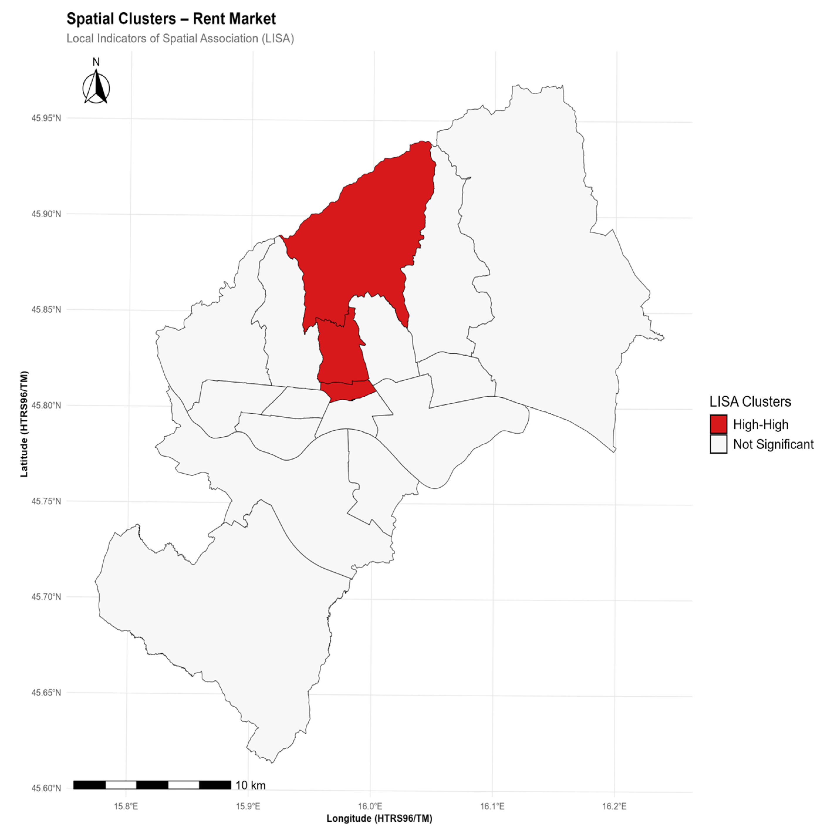
LISA study shows that there are three important High-High clusters: Donji Grad (1369 EUR/month), Gornji Grad-Medvešćak (1502 EUR/month), and Podsljeme (1311 EUR/month). This larger clustering in relation to the sale market supports the idea that rental property has a stronger geographical concentration. The three groups have much in common: they are historic or prestigious neighborhoods with great amenities, good public transportation links, and easy access to job areas. There are not any big Low-Low rent clusters, which is similar to how the sale market works. Figure 7 and Figure 8 show how the rent market works.

5.1.3. Cross-Market Spatial Comparison

Comparing spatial autocorrelation across markets reveals consistent positive dependencies, supporting Hypothesis 3. Both markets exhibit statistically significant positive spatial autocorrelation (p < 0.01), indicating spatial clustering appear to represent a fundamental characteristic of Zagreb housing. However, the magnitude differential; rent market Moran’s I (0.42) substantially exceeding sale market (0.29) suggests spatial dependencies operate with varying intensity across tenure types.

LISA analysis reveals overlapping yet distinct patterns. Donji Grad emerges as High-High in both markets, confirming its premium status across tenure types. However, the rental market exhibits two additional significant clusters absent in sale results, reinforcing inference that spatial concentration operates more intensely in rentals. Figure 9 compares Moran’s I values.

5.2. Spatial Regression Model Comparison

Having established spatial autocorrelation exists, this subsection addresses Research Question 2: Do spatial models improve fit over OLS? Four specifications are compared: OLS baseline, SLX, SAR, SEM, using AIC and R². Differences exceeding 2 AIC units indicate meaningful improvement [53].

5.2.1. Sale Market Model Performance

Table 2. Model comparison-sale market.

Model	AIC	Log Likelihood	R2/Pseudo R2
OLS	246.3097	−118.1548	0.7420
SLX	236.4119	−110.2059	0.8987
SAR	248.2412	−118.1206	0.7431
SEM	248.2736	−118.1368	0.7426
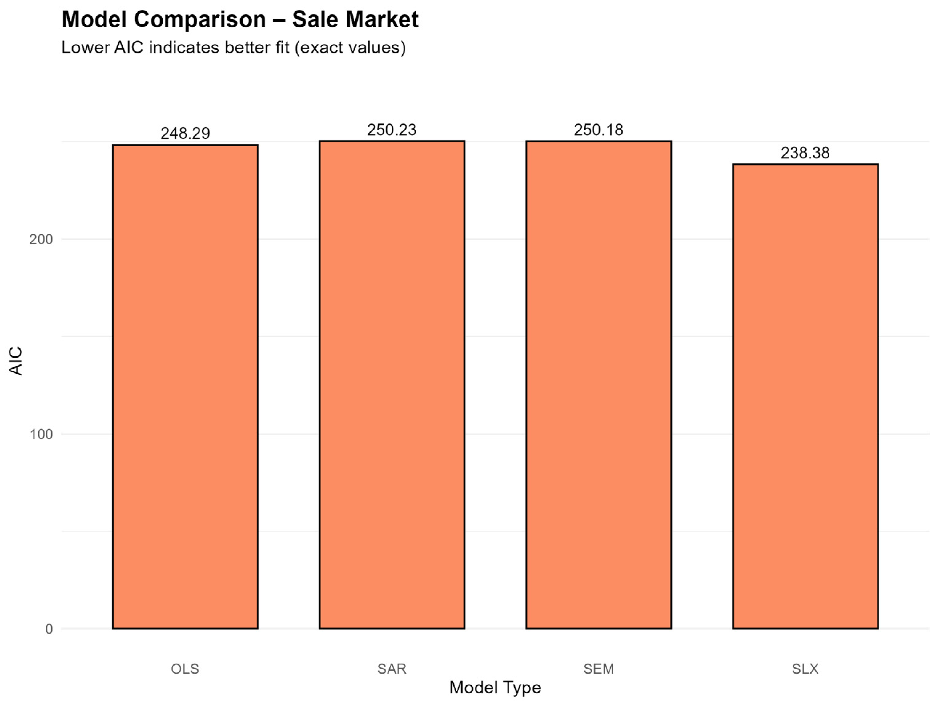
SDM	238.2122	−110.1061	0.8999

presents sale market model comparison using the three-variable specification (Vacancy_Rate, Housing_Density, Avg_Household_Size) adopted following multicollinearity assessment. Five model specifications were estimated: non-spatial OLS baseline and four spatial models (SLX, SAR, SEM, SDM). OLS yields AIC of 246.31 with R² of 0.7420. Among spatial specifications, SLX emerges as best-fitting with AIC of 236.41, representing a 9.90-unit improvement over OLS. This substantial gain exceeds the 2-unit threshold, providing strong support for Hypothesis 2. SLX achieves R² of 0.8987, capturing an additional 15.7 percentage points of variance compared to OLS.

SLX does better than SAR (AIC = 248.24), SEM (AIC = 248.27), and SDM (AIC = 238.21). This shows that local spatial spillovers from the characteristics of nearby districts explain Zagreb sale prices better than other spatial factors. The Spatial Durbin Model, which includes both the spatial lag of the dependent variable (pWy) and the spatial lags of covariates (WXθ), does not do better than the simpler SLX specification (ΔAIC = +1.80). The spatial autoregressive parameter p in SDM is not statistically significant (p = −0.157, p = 0.655). This means that spatial dependency only works through neighborhood characteristics (WX) and not through price feedback effects (Wy). This conclusion suggests that the creation of home prices is influenced by concrete neighborhood spillovers, including shared facilities, infrastructure, and socioeconomic composition, rather than speculative spatial contagion or price interdependence. It is important to note that not all spatial specifications are better than OLS. SAR (AIC = 248.24) and SEM (AIC = 248.27) do about the same as or worse than the non-spatial baseline (AIC = 246.31). This shows that spatial dependency does not work through price feedback effects (Wy) or unobservables that are spatially correlated (Wu). Only SLX, which includes spillovers from nearby district characteristics (WX), shows a big improvement (ΔAIC = 9.90). This shows that spatial dependencies in Zagreb housing are real neighborhood impacts, not just price contagion or measurement errors.

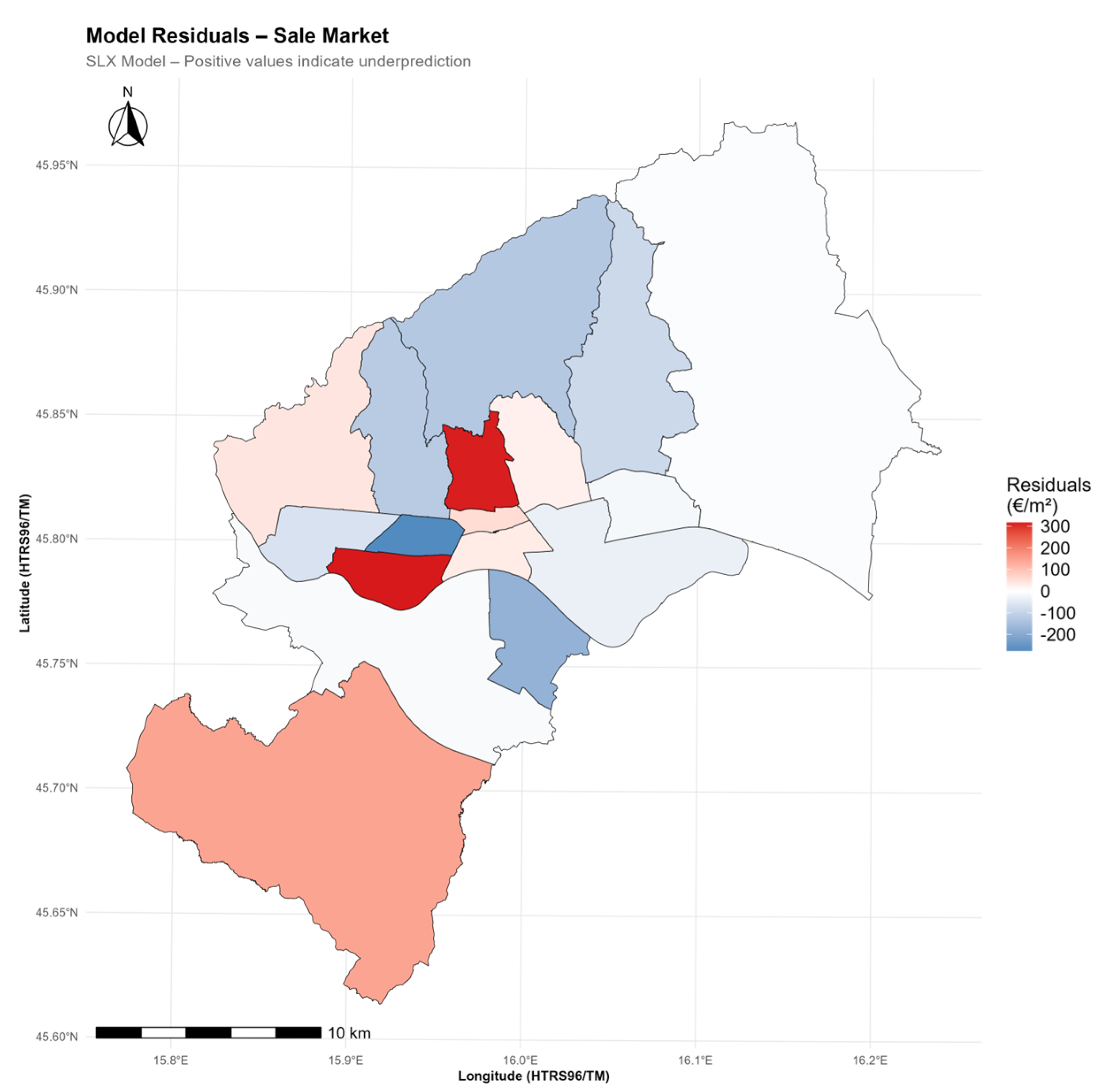
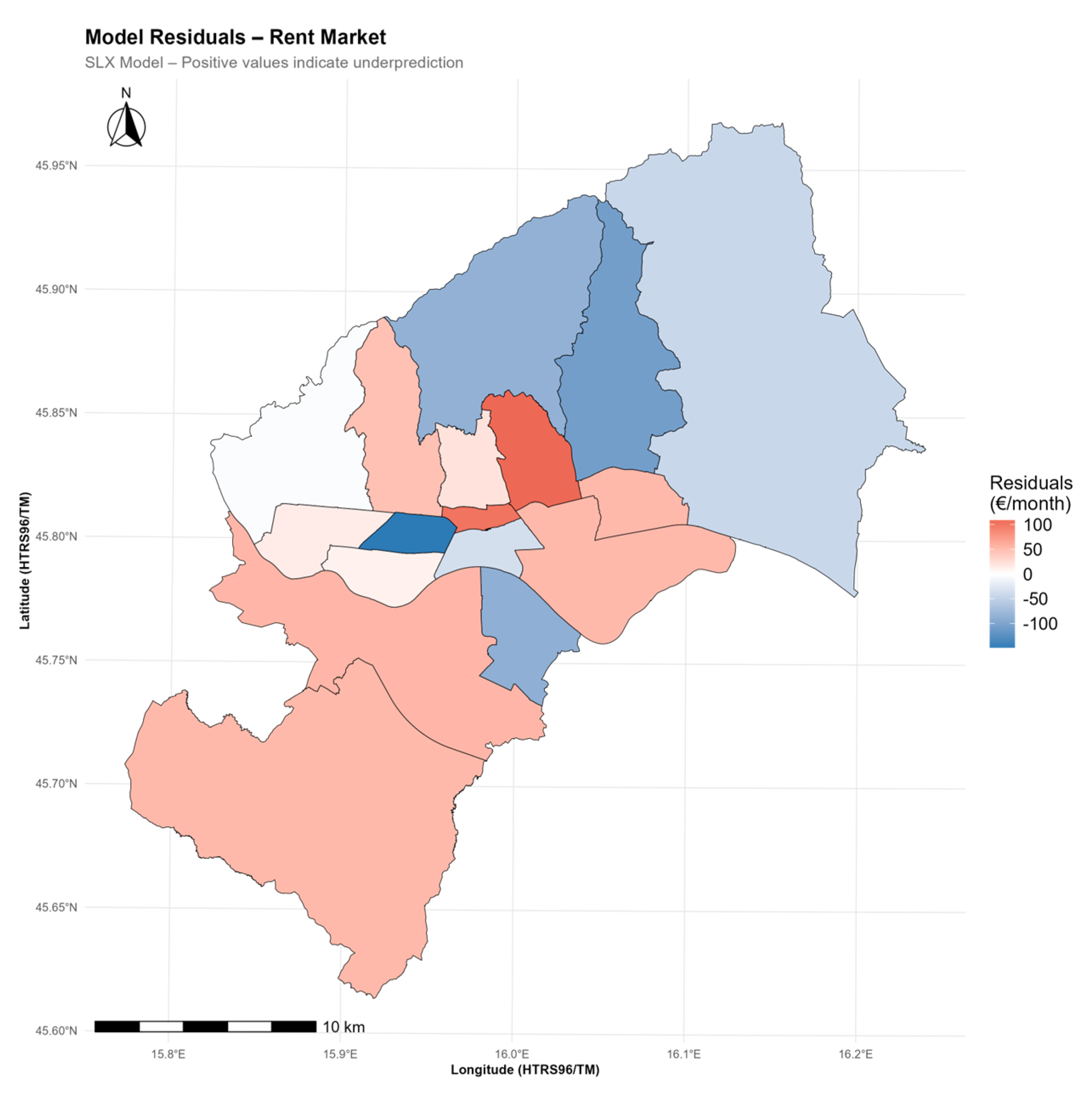
The three-variable specification gets rid of multicollinearity (the highest VIF goes down to 2.55) while still being able to explain a lot. Figure 10 and Figure 11 provide a chart that compares models and the size of the residuals.

5.2.2. Rent Market Model Performance

Table 3. Model comparison-rent market.

Model	AIC	Log Likelihood	R2/Pseudo R2
OLS	233.6287	−110.8143	0.7039
SLX	213.4296	−96.7148	0.9436
SAR	227.1372	−106.5686	0.8203
SEM	233.5104	−109.7552	0.7386
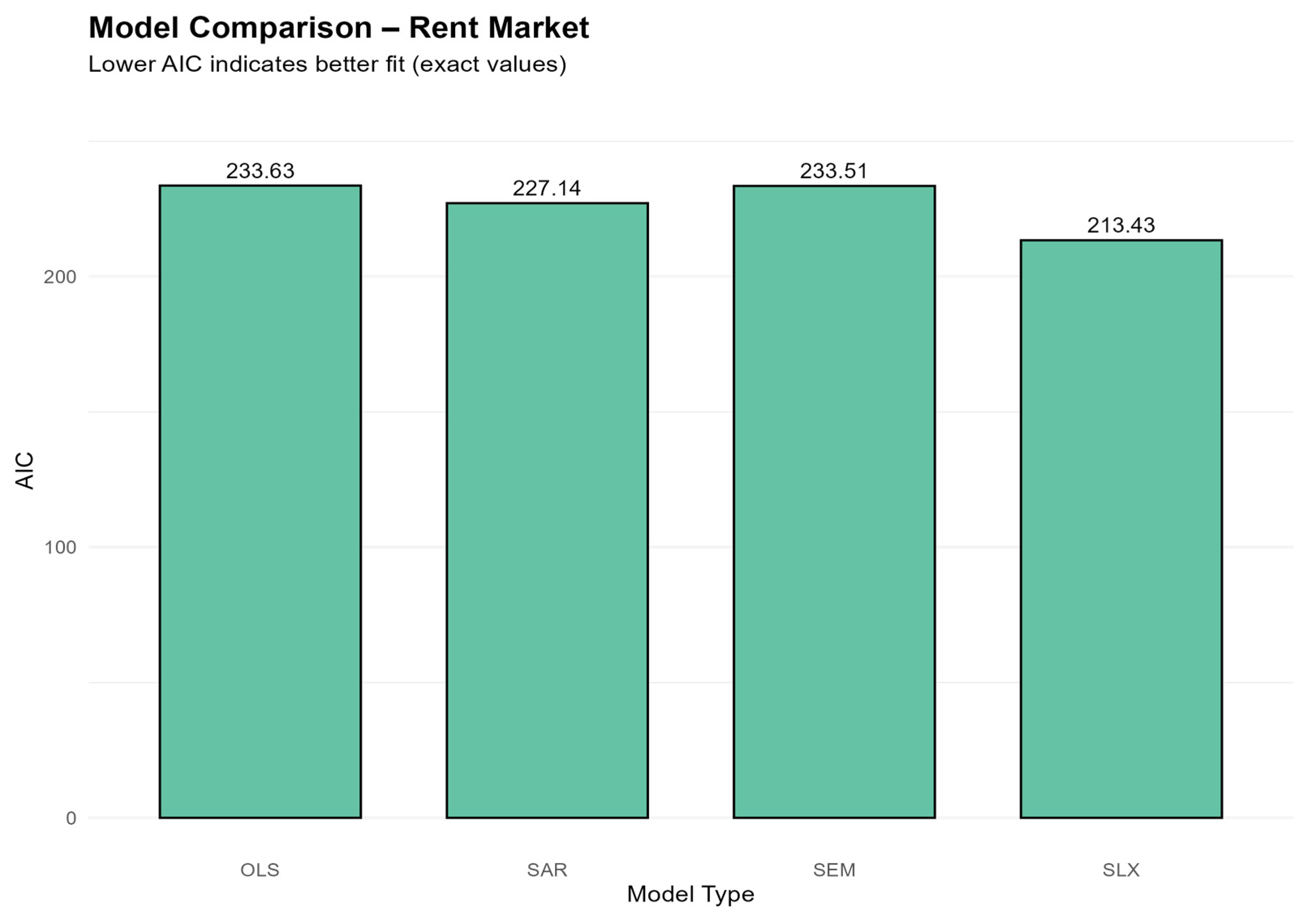
SDM	215.4170	−96.7085	0.9437

shows a comparison of rent market models that use the four-variable specification (Private_Ownership_Pct, Vacancy_Rate, Housing_Density, Avg_Household_Size) that was preserved after checking for multicollinearity. The Akaike Information Criterion for Ordinary Least Squares is 233.63, while the coefficient of determination is 0.7039. The SLX model fits the best among spatial specifications, with an AIC of 213.43. This is a 20.20-unit improvement over OLS, which is more than double the improvement found in the selling market (ΔAIC = 9.90). The increase in pseudo-R² to 0.9436 strongly supports Hypothesis 2 in the rental market, with spatial spillover effects adding an extra 24.0 percentage points of variance.

The higher spatial autocorrelation (Moran’s I = 0.42 compared to 0.29 for sales) in Section 5.2.2 matches the higher geographical modeling benefits. When geographical dependencies are more important, modeling them directly leads to bigger improvements. SLX beats SAR (AIC = 227.14), SEM (AIC = 233.51), and SDM (AIC = 215.42), which is what sales market data says. The Spatial Durbin Model incorporates both the spatial lag of the dependent variable (pWy) and the spatial lags of covariates (WXθ); nonetheless, it does not improve upon the more concise SLX specification (ΔAIC = +1.99). The spatial autoregressive parameter p in the Spatial Durbin Model (SDM) is not statistically significant. This means that neighborhood characteristics (WX) are what make spatial dependency work, not price feedback effects (Wy). This pattern is similar to the sales market, which means that rental prices in Zagreb are affected by real neighborhood spillovers, such as shared services, infrastructure, and socioeconomic makeup, rather than by speculative spatial contagion. The four-variable model includes both Private_Ownership_Pct and Vacancy_Rate, even though the VIF is large (≈18). This is because sensitivity analysis showed that leaving out either variable made the model fit much worse (ΔAIC > 12). Figure 12 and Figure 13 show how models compare and what is left over. In the sales market, SAR (AIC = 227.14) and SEM (AIC = 233.51) do not considerably improve the performance of OLS (AIC = 233.63). SEM’s performance is basically the same as the baseline’s. Only SLX (AIC = 213.43) shows a substantial improvement (ΔAIC = 20.20), which shows that spatial dependencies only work through neighborhood characteristic spillovers (WX) and not through any other spatial mechanisms.

5.2.3. Cross-Market Model Comparison Summary

Cross-market comparison looks at whether spatial characteristics including spatial autocorrelation, model performance rankings, and spatial processes are the same in both market sectors. Sale prices are in EUR/m², whereas rental rates are in EUR/month. This is because buyers care more about the value of the unit and renters care more about the monthly cash flow. These differing units make it impossible to directly compare the sizes of the coefficients, but they do not change how we analyze spatial patterns or how we evaluate model performance. Model comparison measures (Moran’s I, AIC improvements, best-fitting specifications) are consistent across markets, irrespective of pricing units.

Table 4. Cross-market comparison summary.

Market	Moran’s I	p-Value	Best Model	AIC Improvement	Significant
Sale	0.2924	0.0073	SLX	9.90	Yes
Rent	0.4219	0.0005	SLX	20.20	Yes

shows the main outcomes from all the marketplaces. Cross-market comparison shows three patterns that are always the same, which strongly supports the concept. To begin with, both markets show statistically significant positive spatial autocorrelation (H1 supported). The rental market shows higher clustering (Moran’s I = 0.42 vs. 0.29, both p < 0.01). Second, spatial models are much better than OLS in both segments (H2 supported), with AIC increases of 9.90 (sell) and 20.20 (rent). Third, SLX is the best-fitting specification in both markets, which suggests that neighborhood spillovers are the main way that spatial dependency works. The fact that SLX is better than more complicated specifications, like the Spatial Durbin Model (SDM), which includes both the spatial lag of the dependent variable and the spatial lags of covariates, shows that spatial dependence only works through neighborhood characteristics (WX) and not through price feedback effects (Wy). The fact that this is true in all markets, even if the variable specifications are different (three variables for sale, four for rent), shows that spatial spillover effects are strong in Zagreb’s housing market.

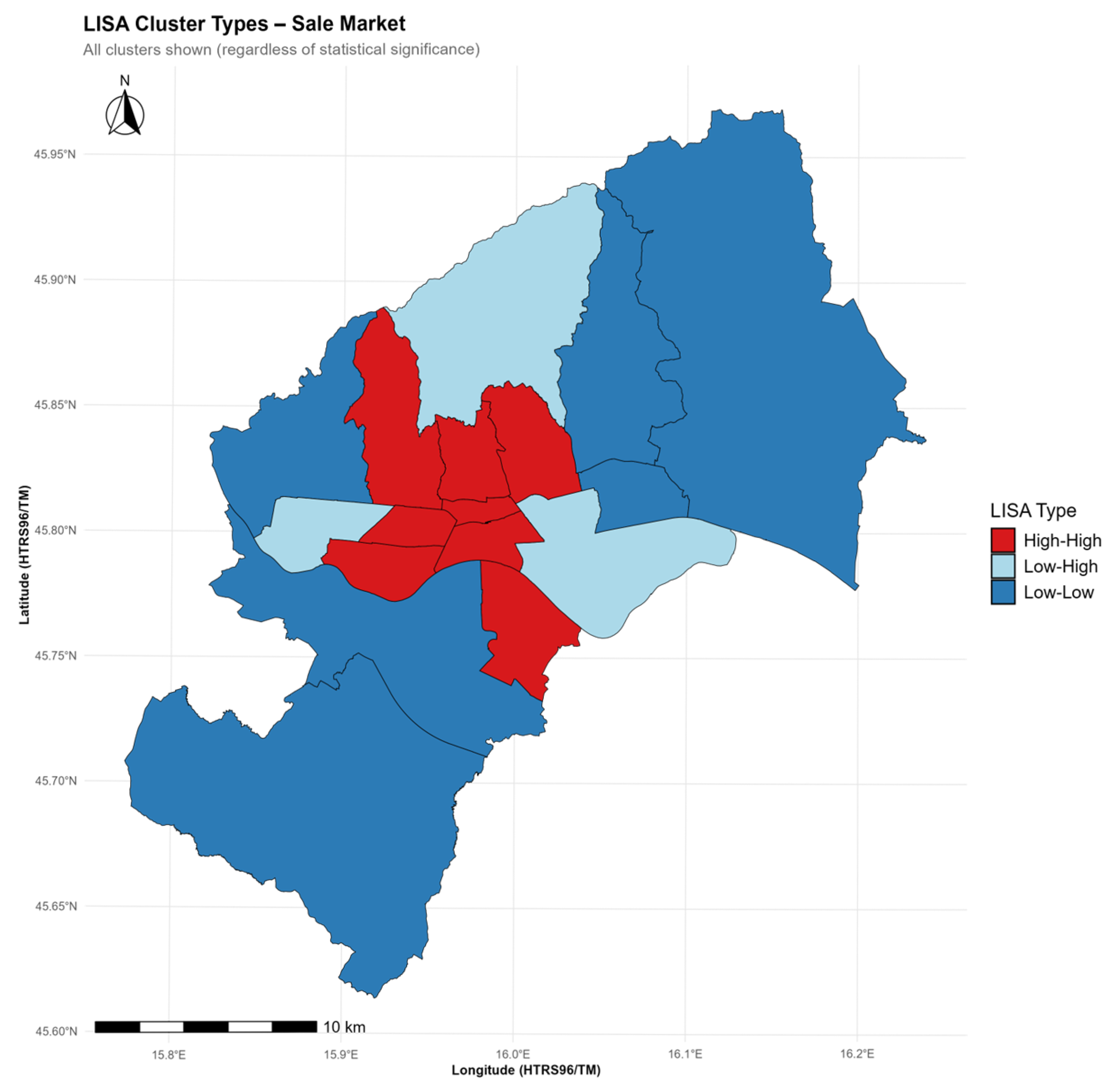
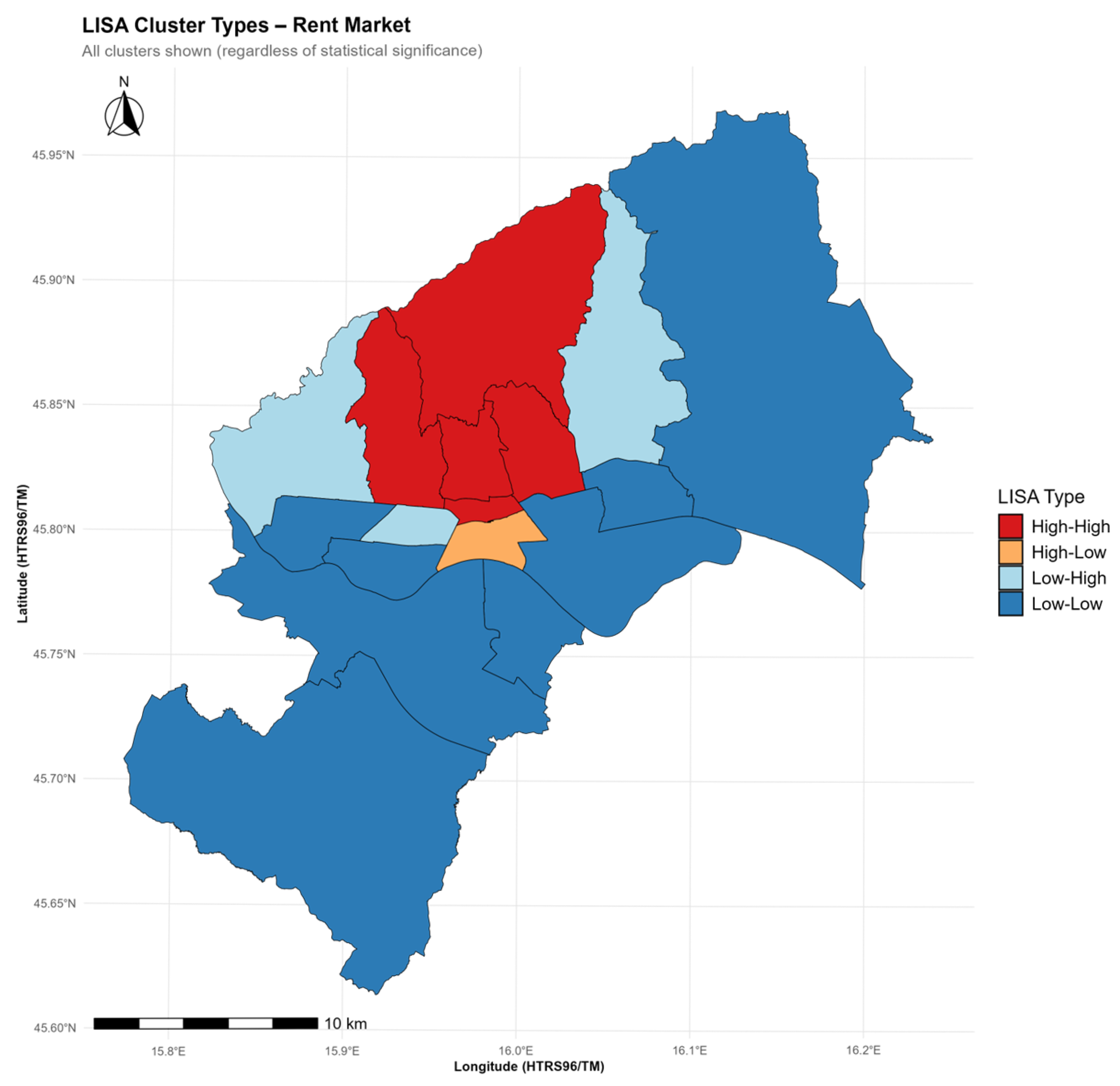
The rental market has larger gains in a systematic way. For example, it has more spatial autocorrelation (Moran’s I = 0.42 vs. 0.29) and greater model improvement (ΔAIC = 20.20 vs. 9.90). This shows that rental housing has more distinct spatial structure than owner-occupied housing. This difference could be due to the fact that rental properties are mostly located in easily accessible central areas, landlords use spatial comparison tactics to set asking prices, or tenants move about a lot, which makes them more sensitive to neighborhood features and services. Figure 14 and Figure 15 illustrate LISA cluster classifications for all sorts of districts, regardless of whether they are statistically significant. This shows the full spatial structure of home pricing patterns. These maps add to Figure 6 and Figure 8, which only show statistically significant clusters at p < 0.05, by showing weak or nascent spatial patterns that do not exceed the significance threshold but nonetheless add to the overall spatial context. In the sale market (Figure 14), the central districts make up a continuous High-High cluster that is flanked by Low-High transition zones. The outer districts are mostly Low-Low. The rental market (Figure 15) has a structure that is comparable to the core-periphery model, but the High-High cluster in the north-central area is larger and the types of clusters are more clearly defined. This is in line with the increased spatial autocorrelation found in this segment.

5.3. Full Model Specification and Coefficients

Table 5. Full regression results-SLX model (best-fitting specification) ¹.

		Sale Market (3 Variables)			Rent Market (4 Variables)
Variable	Coefficient	Std. Error	p-Value	Coefficient	Std. Error	p-Value
(Intercept)	−2070.2687	2576.7732	0.4404	−43,459.0882	9658.6572	0.0020
Vacancy_Rate	−26.0906	30.2776	0.4090	239.3825	50.0990	0.0014
Housing_Density	−0.0277	0.0325	0.4149	−0.0251	0.0173	0.1845
Avg_Household_Size	−768.2643	285.2498	0.0226	−194.9609	144.2604	0.2135
Private_Ownership_Pct	—	—	—	88.7209	25.2602	0.0079
lag.Vacancy_Rate	246.8954	66.6730	0.0041	759.3253	160.9668	0.0015
lag.Housing_Density	0.2591	0.1067	0.0356	−0.0195	0.0544	0.7293
lag.Avg_Household_Size	1181.0986	650.5212	0.0995	277.0882	341.1541	0.4402
lag.Private_Ownership_Pct	—	—	—	333.1774	83.5372	0.0040

¹ Sale market prices measured in EUR/m² (unit value); rental market prices measured in EUR/month (monthly cash flow). Different units reflect natural market conventions and preclude direct comparison of coefficient magnitudes across markets.

shows all of the regression results for the best SLX models in both markets. This includes all of the coefficient estimates, standard errors, and significance tests. The table shows distinct patterns of direct impacts (characteristics of the own district) and geographical spillover effects (spatially delayed variables, WX terms) across different types of housing. In the sales market (three-variable specification), the vacancy rate has a small but negative direct effect (β = −26.09, p = 0.409). On the other hand, its spatial lag shows a strong positive and significant effect (β = 246.90, p = 0.004). This pattern suggests that districts with high vacancy rates do not always have lower prices. However, districts next to neighborhoods with high vacancy rates tend to have higher prices. This is probably because there is a difference between central districts with lots of amenities and functional vacancy (turnover, investment properties) and peripheral areas with structural vacancy (abandonment, disinvestment). Housing density has a small direct effect (β = −0.028, p = 0.415) but a big positive spatial spillover (β = 0.259, p = 0.036). This fits with the idea that agglomeration economies work at the neighborhood level instead of in separate districts. The average household size shows a significant negative direct influence (β = −768.26, p = 0.023), which means that districts with bigger households had lower sale prices. On the other hand, it has a positive spatial lag coefficient (β = 1181.10, p = 0.099), which means that living near family-oriented communities leads to amenity spillovers related to school quality, safety, and community infrastructure. In the rental market (four-variable specification), the proportion of private ownership is preserved despite multicollinearity due to its substantial influence on model fit. The variable shows strong direct (β = 88.72, p = 0.008) and spatial lag effects (β = 333.18, p = 0.004). This means that districts with higher ownership rates charge higher rents, and being close to neighborhoods with a lot of ownership increases this premium. This is consistent with the idea that owner-occupied areas are more stable and of better quality. The vacancy rate has a strong positive direct effect on the rental market (β = 239.38, p = 0.001), which is the opposite of what is happening in the sales market. It also has a strong positive spatial lag (β = 759.33, p = 0.002). This means various rental markets see vacancy differently. A high vacancy rate could mean that there is a lot of rental supply and tenant preference, especially in central areas where rental demand is high. As shown in earlier sections, the rental market has higher spatial autocorrelation (Moran’s I = 0.42 vs. 0.29) and better model improvement (ΔAIC = 20.20 vs. 9.90). This means that this market segment has a more marked geographical organization. The differing patterns of direct and geographical lag effects in different markets underscore the importance of spatial econometric modeling. If you only look at direct impacts using regular OLS models, you will not see or understand the neighborhood spillover processes that explain most of the variation (R² enhancement: +15.7 percentage points for sales, +24.0 percentage points for rentals). The SLX specification shows that housing prices are affected not only by the characteristics of their own districts but also, and more importantly, by the characteristics of nearby districts. This backs up the idea that spatial dependencies are important parts of urban housing markets. It is important to note that spatial lag coefficients (WX terms) are more likely to be statistically significant than direct impacts. The vacancy rate is significant in both markets (p < 0.01); however, the direct vacancy rate is not significant in sales (p = 0.409). This tendency, where local factors have a bigger effect on house prices than district factors, shows how important spatial spillover effects are in setting home prices. The SLX model fits better mainly because it can show linkages between districts instead of just adding more factors.

5.4. Model Diagnostics and Validation

Diagnostic tests evaluate whether key regression assumptions hold for the best-fitting SLX models. For the sale market, the Shapiro–Wilk test yields W = 0.9386 (p = 0.3024), failing to reject normality; the Breusch–Pagan test produces BP = 5.1766 (p = 0.1593), detecting no significant heteroscedasticity. Rent market diagnostics yield Shapiro–Wilk W = 0.9434 (p = 0.3603) and Breusch–Pagan BP = 4.8479 (p = 0.3033), both failing to reject null hypotheses. These results provide reassurance that both models remain reliable despite the small sample size (n = 17). In summary, results provide consistent support for all three hypotheses. Housing prices exhibit significant positive spatial autocorrelation in Zagreb (H1), with rental markets displaying stronger clustering than sales (Moran’s I = 0.42 vs. 0.29). Spatial regression models, particularly SLX, substantially outperform OLS (H2), with AIC improvements of 9.90 (sale) and 20.20 (rent). These patterns prove consistent across both markets (H3), though operating with greater intensity in rentals. The superiority of SLX over more complex specifications including SDM demonstrates that spatial dependence operates through neighborhood characteristics (WX) rather than price feedback effects (Wy). Diagnostic tests confirm model reliability despite small sample constraints. These findings establish that spatial dependencies constitute fundamental features of Zagreb housing requiring explicit spatial econometric modeling.

6. Discussion

6.1. Interpretation of Key Findings

Moran’s I = 0.29 sale, 0.42 rent shows that neighborhood location is an essential factor in setting prices, along with the features of the property itself. The rental market is probably more clustered because of a few things: rental properties are more likely to be in central locations that are easy to get to and have a lot of tenant demand; landlords use more direct spatial comparisons when setting rents; and Zagreb’s small rental market, which was shaped by mass privatization that created super-homeownership over 90%, has a higher spatial concentration than the dispersed owner-occupied inventory.

The SLX specification’s consistent superiority offers essential insights into spatial mechanics. There were three types of spatial dependence tested: (1) spatial lag of the dependent variable (SAR), which shows how prices affect each other; (2) spatial error correlation (SEM), which shows how missing spatially structured variables affect each other; and (3) spatial lags of covariates (SLX), which shows how neighborhood characteristics spill over. Only SLX did far better than OLS in both sectors (ΔAIC = 9.90 sale, 20.20 rent), while SAR and SEM did around the same as or worse than the non-spatial baseline. This pattern shows that spatial dependencies in Zagreb housing are caused by real neighborhood effects from the features of nearby districts, not by price contagion (SAR) or omitted variable bias (SEM).

Prices for residences in Zagreb are more affected by things like vacancy patterns, household composition, density, and ownership structure than by prices in adjacent areas. The insignificance of the spatial autoregressive parameter p in SDM (p > 0.05 in both markets) confirms that geographical clustering indicates authentic amenity spillovers rather than speculative price contagion or measurement inaccuracies.

According to the LISA study, the costliest cluster in both markets is Donji Grad, which is where most of the High-High clusters are located. Monocentric urban models indicate that prices go down as you move away from big cities. This fits with that idea. There may not be a lot of Low-Low clusters at the district level because Zagreb is tiny or because the aggregation hides smaller areas with a lot of cheap housing.

6.2. A Comparison with Other Research

The geographical autocorrelation values for Zagreb are in the same range as those for other European cities, but they are on the lower end for sale marketplaces. Paris had a Moran’s I value of more than 0.40, while cities in Norway had an average value of about 0.31. Zagreb’s low selling market value is probably due to the city’s smaller size, the fact that values are averaged across different locations at the district level, and the fact that the city has unique post-socialist housing legacies that create unique spatial patterns.

It is helpful to compare this study to others done in Central and Eastern Europe. Using property-level data, Krakow rentals showed more spatial autocorrelation (I = 0.50), which suggests that higher resolution shows more clustering. But at the district level, Zagreb’s rental market value (I = 0.42) is still high, which shows that there is a strong spatial structure even at a lower resolution. The improvements to the model; AIC reductions of 9.90 for sales and 20.20 for rent, are much higher than what is usually considered acceptable and are in line with what has been found in research from Western Europe. SLX’s constant supremacy is different from Western European research, which usually finds SAR or Spatial Durbin specifications to be the best. Zagreb’s SLX dominance may be due to unique socialist-era planning that made relatively separate housing zones with slow, gradual changes. This caused local spillovers in nearby areas without substantial global spatial multiplier effects.

6.3. The Housing Situation After Socialism

This study improves understanding of housing dynamics in post-socialist cities by demonstrating that spatial dependencies operate throughout Central and Eastern Europe, despite differing institutional histories. Mass privatization led to super-homeownership systems that are substantially different from the mixed-tenure markets in Western Europe. Zagreb’s spatial patterns, on the other hand, reflect more complicated relationships. Dependencies work like Western cities, with accessibility gradients and neighborhood impacts. However, they are distinct due to the post-socialist institutional structure. A high vacancy rate (an average of 17.8% compared to 5–10% in Western Europe) means that people are holding their investment homes. This is a one-of-a-kind design that modifies how supply and demand work. The rental market’s higher spatial autocorrelation may be because rental properties are often clustered together in certain neighborhoods, while homes that are owned and lived in are more spread out. The significant impact of housing density on neighborhoods demonstrates that the planning concepts from the socialist era continue to influence contemporary living conditions.

6.4. Policy Implications

Spatial econometric methods are necessary for accurate valuation, forecasting, and policy assessment in the housing market. You make a specification mistake if you treat observations as separate. Policies that cut down on vacancies, urban regeneration projects, or improvements to infrastructure can help the overall neighborhood by making it easier to get around and making people feel like the community is better. Policymakers should keep these spatial multipliers in mind when they make decisions. People are curious about how fair housing is in different locations because there are so many High-High clusters in key districts. This study cannot definitively ascertain causation; however, the observed patterns suggest that housing policy should consider both the total supply and the spatial dimensions of affordability. The rental market’s superior spatial organization suggests that rental housing policy needs to pay close attention to how space is divided up and how it affects neighborhoods.

6.5. Limitations and Future Directions

The limited sample size (n = 17 districts) constrains statistical power and coefficient precision. Methodological research, conversely, indicates that spatial dependence tests remain effective with n = 20–30 when appropriate frameworks are employed. District-level aggregation focuses more on following administrative borders and getting to Census 2021 data than on resolution, data quality, and policy relevance. Future research should employ finer spatial resolution at the neighborhood or property level, as larger samples enable comprehensive spillover analysis. Using published asking prices instead of transaction prices makes things less clear. Negotiation margins suggest that the prices people ask for are usually 5–15% higher than the prices they pay. But study demonstrates a strong correlation (r > 0.95) between asking and transaction costs in cross-sectional analysis, which means that relative spatial patterns still remain. It would be easier to check if you compared it to land registration transaction data. Cross-sectional design makes it harder to draw conclusions about cause and effect. The research indicates the presence of spatial autocorrelation and an improved model fit; nevertheless, it does not definitively identify the causal mechanisms. By tracking panel data over time, dynamic spatial models could tell the difference between present correlations and causal spillovers. They could also include fixed effects to account for features that do not vary over time. The simple model with four control variables has to leave out other important things. Variable selection gives priority to the availability of Census 2021 data at the district level and its theoretical relevance. This ensures that the data is of high quality and that administrative boundaries are correct. Adding school quality, distance to public transportation, green space, and environmental amenities to future research will strengthen the findings. The geographically lagged covariates in the SLX model address issues with omitted variables by integrating unmeasured spatially structured spillovers. This study makes it clear how geography affects Zagreb, but if it were done in other Croatian cities, it would be possible to compare the results to see if they are unique to Zagreb or if they are more general Croatian traits. Subsequent research using larger samples should incorporate the assessment of spillover effects through direct, indirect, and total impact decompositions. To see how things, evolve over time, this will need both greater sample sizes and panel data. This study makes a big contribution by showing that spatial dependency is an important feature of Zagreb housing that needs accurate spatial econometric modeling, even though it has some flaws. Documented patterns are stable across different marketplaces, specifications, and general empirical regularities. This sets the stage for the next round of study, which will use better data and more advanced methods to fix the problems that have been found.

7. Conclusions

This study represents the intra-urban spatial econometric analysis of Zagreb’s housing market. While previous studies on Zagreb’s housing market have applied hedonic OLS frameworks incorporating distance and location variables, they have not explicitly addressed spatial autocorrelation nor compared spatial econometric specifications [30]. Combining data from the 2021 Census with prices advertised in Zagreb’s 17 city districts shows that geographical dependencies are important features of urban property markets in Central and Eastern Europe after socialism.

7.1. Key Findings

Three significant empirical findings emerge. First, housing prices show statistically substantial positive spatial autocorrelation (H1 supported): Global Moran’s I = 0.29 for sales (p = 0.007) and 0.42 for rentals (p < 0.001). This means that there is a lot of spatial clustering, with rental markets showing stronger structuring. LISA research shows that Donji Grad is a High-High cluster in both markets. Rentals also show other notable clusters. The lack of Low-Low clusters means that affordable housing does not group together in areas that are close to each other at the district level.

Second, spatial models do a lot better than OLS (H2 supported). With AIC gains of 9.90 (sales) and 20.20 (rentals), SLX is the best-fitting specification in both markets. This is much beyond the 2-unit threshold for substantial improvement. SLX gets R² of 0.899 for sales and 0.944 for rentals, which is 15.7 and 24.0 percentage points more than OLS. SLX is better than the more complicated Spatial Durbin Model (SDM) because the spatial autoregressive parameter p is not important in either market. This shows that spatial dependency works through neighborhood qualities (WX) instead of price feedback effects (Wy). This means that there are real amenity spillovers instead of price contagion.

Third, spatial patterns are strong in both markets (H3 supported), but they are stronger in rentals. There is a lot of spatial autocorrelation and modeling improvements in both segments. This shows that geographical dependencies are structural aspects of Zagreb housing, not just something that happens in one segment. The Shapiro–Wilk and Breusch–Pagan tests show that the model is reliable even though the sample size is modest (all p > 0.15). The residual analysis also shows that the SLX specifications do a good job of capturing systematic spatial variation. Spatial regression model comparison revealed that only one spatial mechanism spillover from neighboring district characteristics (SLX); substantially improved upon non-spatial OLS. Alternative specifications incorporating price feedback effects (SAR) or spatially correlated errors (SEM) did not outperform the baseline, demonstrating that spatial dependencies reflect tangible neighborhood effects rather than price contagion or measurement artifacts.

7.2. Contributions and Implications

This study adds to what we already know in three ways. First, it fills a major research vacuum by being the formal spatial econometric study of intra-urban housing trends in Zagreb. This study lays the groundwork for spatial dependencies as key market characteristics. Second, it helps us understand how housing works in post-socialist countries by showing that spatial dependencies work in Central and Eastern Europe even though the institutions there have different histories, such as mass privatization, super-homeownership (>90%), high vacancy rates, and inherited socialist spatial configurations. The results show that urban economic basics (such accessibility gradients, amenity capitalization, and neighborhood effects) cause spatial clustering in post-socialist cities that is similar to patterns seen in the West. However, path-dependent institutional contexts affect how these dependencies show up. Third, it shows methodological insights for spatial econometrics in data-limited settings: when the right specifications are used, meaningful patterns show up with n = 17 districts, showing that careful alignment of census and administrative data makes it possible to do rigorous analysis even with a small sample size. Documented spatial connections have immediate consequences for policy and practice. Spatial econometric methods are needed for housing market analysis, whether it is for valuation, forecasting, or policy evaluation, to prevent making mistakes in the specification. Housing policy interventions provide neighborhood-wide impacts via local spillovers; expenditures in infrastructure, urban renewal, or programs aimed at reducing vacancies benefit adjacent neighborhoods, necessitating that policymakers consider spatial multipliers. The concentration of High-High clusters in central districts raises questions about spatial equity. This means that housing policy should take into account spatial dimensions of affordability as well as overall supply, especially for rental housing where spatial structuring is more obvious.

7.3. Future Research Direction

This basic study opens up many new areas of research, such as using land registry data to check transaction prices; doing finer spatial resolution analysis to get larger samples and more accurate spillover measurements; using panel data approaches to follow districts over time to find causal mechanisms; adding more control variables like amenities, infrastructure, and environmental quality; testing the robustness of different spatial weights; and comparing the results with those of other Croatian cities to see if they can be applied to other places. Future studies should look into the fundamental mechanisms: What causes rental housing to cluster more strongly? How do the planning legacies of the communist era still affect the way things are done today? To answer these problems, you need to use both quantitative geographical analysis and qualitative study on how decisions are made and how institutions change over time. In conclusion, spatial dependencies are important parts of Zagreb’s housing market that need to be modeled in a clear way in order to be analyzed correctly. The significant enhancements to the model shown herein; despite the limited sample size illustrate that spatial methodologies are not only theoretical advancements but vital instruments for comprehensive real estate analysis in Croatia’s capital. The results are in line with broader patterns seen in Western European cities, but they also show how post-socialist contexts are different. This gives a strong empirical basis for spatial housing analysis that is directly useful to market participants and policymakers.

References

1. Anselin, L. Spatial Econometrics: Methods and Models; Kluwer Academic Publishers: Dordrecht, The Netherlands, 1988. [Google Scholar]
2. Dubin, R.A. Spatial autocorrelation: A primer. J. Hous. Econ. 1998, 7, 304–327. [Google Scholar] [CrossRef] [Scilit]
3. Moran, P.A.P. Notes on continuous stochastic phenomena. Biometrika 1950, 37, 17–23. [Google Scholar] [CrossRef] [Scilit] [PubMed]
4. Anselin, L.; Bera, A.K. Spatial dependence in linear regression models with an introduction to spatial econometrics. In Handbook of Applied Economic Statistics; Ullah, A., Giles, D.E., Eds.; Marcel Dekker: New York, NY, USA, 1998; pp. 237–289. [Google Scholar]
5. Osland, L. An application of spatial econometrics in relation to hedonic house price modeling. J. Real Estate Res. 2010, 32, 289–320. [Google Scholar] [CrossRef] [Scilit]
6. Baumont, C.; Legros, D. Neighborhood effects in spatial housing value models: The case of the metropolitan area of Paris (1999). Pap. Reg. Sci. 2009, 88, 751–774. [Google Scholar]
7. Égert, B.; Mihaljek, D. Determinants of house prices in Central and Eastern Europe. Comp. Econ. Stud. 2007, 49, 367–388. [Google Scholar] [CrossRef] [Scilit]
8. Tomal, M. Modelling housing rents using spatial autoregressive geographically weighted regression: A case study in Cracow, Poland. ISPRS Int. J. Geo-Inf. 2020, 9, 346. [Google Scholar] [CrossRef] [Scilit]
9. Getis, A.; Ord, J.K. The analysis of spatial association by use of distance statistics. Geogr. Anal. 1992, 24, 189–206. [Google Scholar] [CrossRef] [Scilit]
10. Anselin, L. Local Indicators of Spatial Association—LISA. Geogr. Anal. 1995, 27, 93–115. [Google Scholar] [CrossRef] [Scilit]
11. Anselin, L.; Bera, A.K.; Florax, R.; Yoon, M.J. Simple diagnostic tests for spatial dependence. Reg. Sci. Urban Econ. 1996, 26, 77–104. [Google Scholar] [CrossRef] [Scilit]
12. LeSage, J.; Pace, R.K. Introduction to Spatial Econometrics; Chapman & Hall/CRC Press: Boca Raton, FL, USA, 2009. [Google Scholar]
13. Elhorst, J.P. Spatial Econometrics: From Cross-Sectional Data to Spatial Panels; Springer: Berlin/Heidelberg, Germany, 2014. [Google Scholar]
14. Halleck Vega, S.; Elhorst, J.P. The SLX model. J. Reg. Sci. 2015, 55, 339–363. [Google Scholar] [CrossRef] [Scilit]
15. Caudill, S.B.; Manage, N.; Mixon, F.G. Using co-ordinate systems in hedonic housing regressions. Real Estate 2024, 1, 41–64. [Google Scholar] [CrossRef] [Scilit]
16. Buszta, J.; Kik, I.; Maciuk, K. The impact of non-market attributes on the property value. Real Estate 2025, 2, 2. [Google Scholar] [CrossRef] [Scilit]
17. Rüttenauer, T. Spatial regression models: A systematic comparison of different model specifications using Monte Carlo experiments. Sociol. Methods Res. 2022, 51, 728–759. [Google Scholar] [CrossRef] [Scilit]
18. LeSage, J.P.; Pace, R.K. The biggest myth in spatial econometrics. Econometrics 2014, 2, 217–249. [Google Scholar] [CrossRef] [Scilit]
19. Cellmer, R.; Cichulska, A.; Bełej, M. Spatial analysis of housing prices and market activity with the geographically weighted regression. ISPRS Int. J. Geo-Inf. 2020, 9, 380. [Google Scholar] [CrossRef] [Scilit]
20. Olszewski, K.; Waszczuk, J.; Widłak, M. Spatial and hedonic analysis of house price dynamics in Warsaw, Poland. J. Urban Plan. Dev. 2017, 143, 04017009. [Google Scholar] [CrossRef] [Scilit]
21. Trojanek, R.; Głuszak, M. Spatial and time effect of subway on property prices. J. Hous. Built Environ. 2018, 33, 359–384. [Google Scholar] [CrossRef] [Scilit]
22. Źróbek, S.; Cellmer, R.; Kuryj, J.; Belej, M. Housing prices and points of interest in three Polish cities. J. Hous. Built Environ. 2024, 39, 1197–1220. [Google Scholar] [CrossRef] [Scilit]
23. Horváth, Á.; Zubor-Nemes, A.; Elekes, Á. Determinants of housing prices from an urban economic point of view: Evidence from Hungary. J. Eur. Real Estate Res. 2019, 12, 131–148. [Google Scholar] [CrossRef] [Scilit]
24. Horváth, K.; Sik, A. Valuation methods for the housing market: Evidence from Budapest. Acta Oeconomica 2016, 66, 527–546. [Google Scholar] [CrossRef] [Scilit]
25. Hlaváček, P.; Komorníková, M.; Řehová, S.; Šerý, O.; Kočí, V. Spatial pattern of property prices in a post-industrial Czech city: Impact of brownfields. Post-Communist Econ. 2021, 33, 874–897. [Google Scholar]
26. Bălănică, C.; Stănescu, I. The price of dwelling in Bucharest: A hedonic approach to the real estate market. J. Urban Plan. Dev. 2022, 148, 05022033. [Google Scholar]
27. Špirková, D.; Ivanovičová, I.; Kubík, P. Real estate market analysis using spatial data mining. IOP Conf. Ser. Mater. Sci. Eng. 2018, 471, 102056. [Google Scholar]
28. Tsenkova, S. Housing Policy Reforms in Post-Socialist Europe: Lost in Transition; Physica-Verlag: Heidelberg, Germany, 2009. [Google Scholar]
29. Stephens, M.; Lux, M.; Sunega, P. Post-socialist housing systems in Europe: Housing welfare regimes by default? Hous. Stud. 2015, 30, 1210–1234. [Google Scholar] [CrossRef] [Scilit]
30. Slišković, T.; Tica, J. The importance of distance in hedonic housing price model—The case of Zagreb. Ekon. Pregl. 2019, 70, 677–705. [Google Scholar] [CrossRef] [Scilit]
31. Kunovac, D.; Pufnik, A.; Ravnik, R. Indices of Real Estate Prices in Croatia; Working Paper W-20; Croatian National Bank: Zagreb, Croatia, 2008. [Google Scholar]
32. Vizek, M.; Stojčić, N.; Mikulić, J. Spatial spillovers of tourism activity on housing prices: The case of Croatia. Tour. Econ. 2023, 29, 1261–1283. [Google Scholar] [CrossRef] [Scilit]
33. Steier, M. Spatial dependencies in apartment prices. Reg. Stud. Reg. Sci. 2020, 7, 416–420. [Google Scholar]
34. Hochstenbach, C.; Arundel, R. Spatial housing market bifurcation: From boom to bust and back again. Urban Geogr. 2020, 41, 500–521. [Google Scholar]
35. Goodman, A.C.; Thibodeau, T.G. Housing market segmentation and hedonic prediction accuracy. J. Hous. Econ. 2003, 12, 181–201. [Google Scholar] [CrossRef] [Scilit]
36. Tu, Y.; Sun, H.; Yu, S.-M. Spatial autocorrelations and urban housing market segmentation. J. Real Estate Financ. Econ. 2007, 34, 385–406. [Google Scholar] [CrossRef] [Scilit]
37. Arundel, R.; Ronald, R.; Kadi, J. Spatial inequalities in housing: What can we learn from spatial analysis? Urban Geogr. 2024, 45, 203–228. [Google Scholar]
38. Paixão, L.; Seidel da Costa, M.A. Impacts of school quality on apartment market prices: A spatial autoregressive regression approach. Real Estate 2026, 3, 6. [Google Scholar]
39. González, M.A.S.; Erba, D.A. Hedonic price method to measure neighborhood quality in South America. Real Estate 2025, 2, 1. [Google Scholar]
40. Can, A. Specification and estimation of hedonic housing price models. Reg. Sci. Urban Econ. 1992, 22, 453–474. [Google Scholar] [CrossRef] [Scilit]
41. Anselin, L.; Florax, R.J.G.M. Small sample properties of tests for spatial dependence in regression models: Some further results. In New Directions in Spatial Econometrics; Anselin, L., Florax, R.J.G.M., Eds.; Springer: Berlin/Heidelberg, Germany, 1995; pp. 21–74. [Google Scholar]
42. De Paola, P. Real estate valuations with small dataset: A novel method based on the maximum entropy principle and Lagrange multipliers. Real Estate 2024, 1, 26–40. [Google Scholar] [CrossRef] [Scilit]
43. Lyons, R.C. Can list prices accurately capture housing price trends? Insights from extreme market conditions. Financ. Res. Lett. 2019, 30, 228–232. [Google Scholar] [CrossRef] [Scilit]
44. Han, L.; Strange, W.C. What is the role of the asking price for a house? J. Urban Econ. 2016, 93, 115–130. [Google Scholar] [CrossRef] [Scilit]
45. Fotheringham, A.S.; Wong, D.W.S. The modifiable areal unit problem in multivariate statistical analysis. Environ. Plan. A 1991, 23, 1025–1044. [Google Scholar] [CrossRef] [Scilit]
46. Manganelli, B.; De Mare, G.; Nesticò, A. Methodology for mitigating the effect of the Modifiable Areal Unit Problem (MAUP) in the housing density–housing price relationship. J. Hous. Built Environ. 2024, 39, 1831–1848. [Google Scholar]
47. Boeing, G. Online rental housing market representation and the digital reproduction of urban inequality. Environ. Plan. A Econ. Space 2020, 52, 449–468. [Google Scholar] [CrossRef] [Scilit]
48. Bežovan, G. Croatia. In Social Housing in Transition Countries; Hegedüs, J., Lux, M., Teller, N., Eds.; Routledge: London, UK, 2013; pp. 75–91. [Google Scholar]
49. Sýkora, L.; Bouzarovski, S. Multiple transformations: Conceptualising the post-communist urban transition. Urban Stud. 2012, 49, 43–60. [Google Scholar] [CrossRef] [Scilit]
50. Czembrowski, P.; Kronenberg, J. Integrating non-monetary and monetary valuation methods: SoftGIS and hedonic pricing. Ecol. Econ. 2016, 130, 166–175. [Google Scholar] [CrossRef] [Scilit]
51. Bivand, R.S.; Pebesma, E.; Gómez-Rubio, V. Applied Spatial Data Analysis with R, 2nd ed.; Springer: New York, NY, USA, 2013. [Google Scholar]
52. Bivand, R.; Piras, G. Comparing implementations of estimation methods for spatial econometrics. J. Stat. Softw. 2015, 63, 1–36. [Google Scholar] [CrossRef] [Scilit]
53. Burnham, K.P.; Anderson, D.R. Multimodel inference: Understanding AIC and BIC in model selection. Sociol. Methods Res. 2004, 33, 261–304. [Google Scholar] [CrossRef] [Scilit]
Figure 1. Administrative districts of Zagreb.
Realestate 03 00004 g001
Figure 2. Spatial distribution of sale prices.
Realestate 03 00004 g002
Figure 3. Spatial distribution of rent prices.
Realestate 03 00004 g003
Figure 4. Methodological workflow.
Realestate 03 00004 g004
Figure 5. Moran scatterplot-sale market.
Realestate 03 00004 g005
Figure 6. LISA clusters-sale market (significant only).
Realestate 03 00004 g006
Figure 7. Moran scatterplot-rent market.
Realestate 03 00004 g007
Figure 8. LISA clusters-rent market (significant only).
Realestate 03 00004 g008
Figure 9. Cross-Market Moran’s I Comparison.
Realestate 03 00004 g009
Figure 10. Model comparison chart-sale market.
Realestate 03 00004 g010
Figure 11. Residual map-sale market.
Realestate 03 00004 g011
Figure 12. Model comparison chart-rent market.
Realestate 03 00004 g012
Figure 13. Residual map-rent market.
Realestate 03 00004 g013
Figure 14. LISA all clusters-sale market (all clusters).
Realestate 03 00004 g014
Figure 15. LISA all clusters-rent market (all clusters).
Realestate 03 00004 g015