The External Exposome and Life Expectancy: Formaldehyde as a Leading Predictor in U.S. Counties

Abstract

Life expectancy in the United States varies significantly by region, a gap often explained by socioeconomic factors like income and education. However, the relative contribution of atmospheric exposures is less understood. We identify formaldehyde exposure and wet-bulb temperature as leading predictors of county-level life expectancy. Our analysis of 22,540 county-year observations (2012–2019) shows that formaldehyde ranked as the second-strongest predictor, surpassed only by educational attainment. Wet-bulb temperature, a physiological measure of heat stress, ranked sixth and was the leading meteorological predictor. We identified these patterns using XGBoost with SHAP analysis, integrating atmospheric exposures, livestock density, socioeconomic conditions, and smoking prevalence within an external exposome framework. These results suggest that air pollutants and heat stress provide predictive information beyond traditional socioeconomic indicators.

1. Introduction

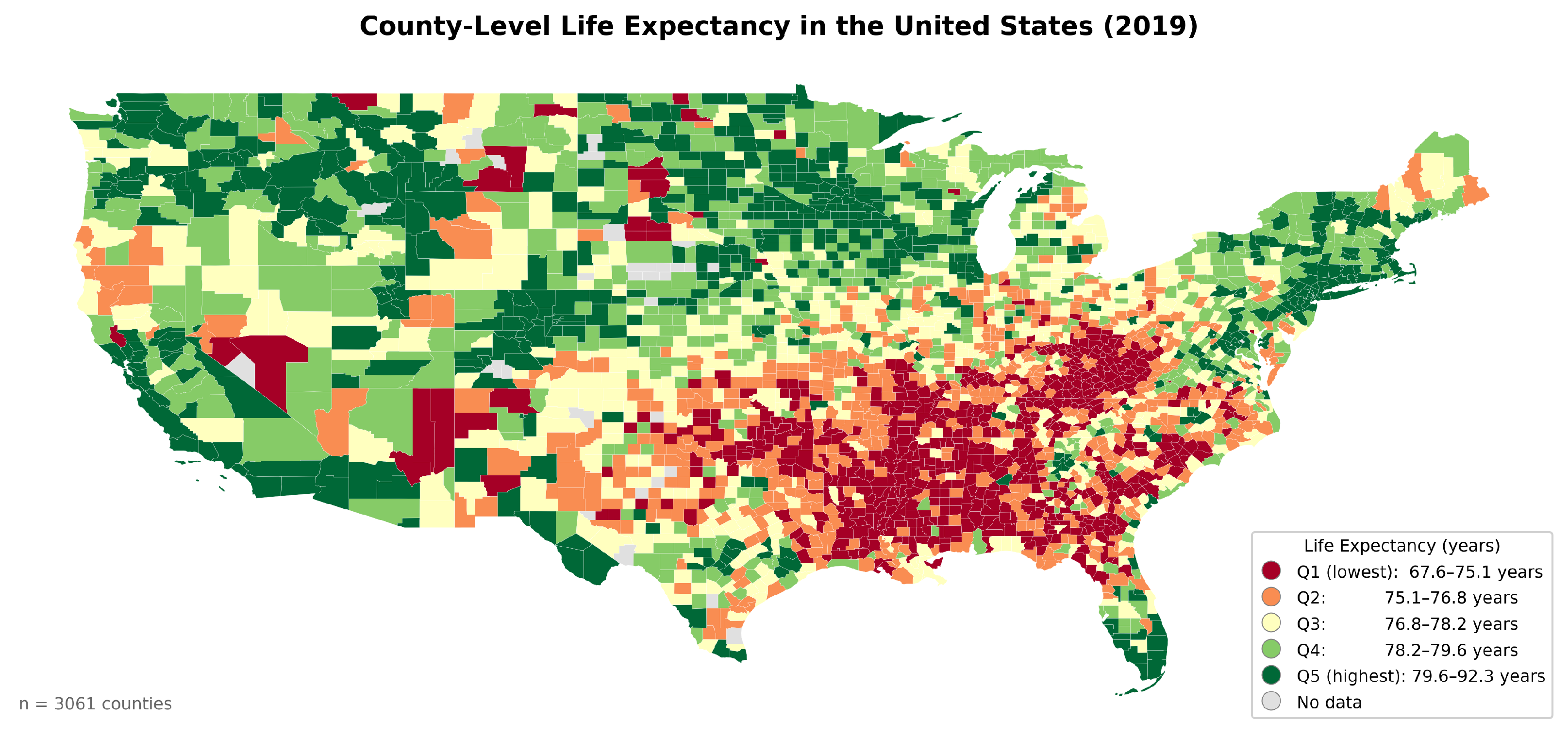
Life expectancy is one of the most widely used indicators of population health, reflecting both the biological aging process and the cumulative effects of social, economic, and environmental determinants. In the United States, persistent disparities in life expectancy across regions, socioeconomic strata, and racial groups have become a growing public health concern [1]. Recent studies have shown that life expectancy can vary by more than a decade between counties with different demographic and environmental profiles, even within the same state [2]. In addition, Americans have shorter life expectancy compared to people in other high-income countries [3], highlighting systemic inequalities that extend beyond individual-level risk factors. These disparities have been linked to a complex interplay of socioeconomic status, racial and ethnic composition, educational attainment, healthcare access, and environmental exposures [4,5]. Figure 1 shows the county-level distribution of life expectancy in 2019.

The socioeconomic determinants of life expectancy are well-established in public health research. Poverty rate, educational attainment, and median household income consistently emerge as powerful predictors of longevity at both individual and population levels [4,5]. Individuals living below the poverty line are more likely to experience adverse living conditions, limited access to healthcare, food insecurity, and higher exposure to environmental hazards [6]. Educational attainment has been shown to have particularly strong correlations with health outcomes. Higher levels of education are associated with increased health literacy, better employment opportunities, higher income, access to social networks, and appreciation of good health behaviors, all of which contribute to improved health outcomes throughout life [7,8]. Smoking is also directly linked to mortality and life expectancy. In a large U.S. study, current smokers lost more than 10 years of life expectancy compared with never smokers [9]. Smoking prevalence is also socially patterned and can overlap with poverty and education [10]. While these socioeconomic and behavioral factors are well-known, their relative importance in the presence of environmental and atmospheric variables remains less understood, particularly when analyzed using modern machine learning approaches that can capture complex, non-linear interactions.

Beyond socioeconomic factors, atmospheric and environmental exposures have also been demonstrated to influence life expectancy in a population. Air quality, in particular, has emerged as a significant determinant, with numerous studies linking elevated levels of environmental pollutants to increased morbidity and premature mortality [11,12]. Studies have linked fine particulate matter (PM_2.5), nitrogen dioxide (NO₂), and ground-level ozone (O₃) exposure to an increased risk of mortality through respiratory and cardiovascular pathways [13,14,15]. Long-term exposure to PM_2.5 has been associated with a shorter life expectancy, with studies estimating that a 10 µg/m³ decrease in PM_2.5 concentration corresponds to approximately 0.61 years of increased longevity [13]. Ozone exposure has similarly been linked to elevated mortality from respiratory causes, with risk increasing by up to 4% for each 10 ppb increment in average concentration [16]. In addition, formaldehyde exposure has been shown to increase the risks of leukemia and Hodgkin’s disease [17]. Livestock density has been proposed as a proxy for localized air quality degradation through greenhouse gas (GHG) emissions and spread of infectious zoonotic diseases such as avian influenza, Q-fever, and MERS [18]. Pig and cattle houses, in particular, have been shown to emit ammonia (${\mathrm{NH}}_3$), which can degrade local air quality, as well as methane (${\mathrm{CH}}_4$) and nitrous oxide (${\mathrm{N}}_2\mathrm{O}$), both potent greenhouse gases [19,20]. Existing studies have typically examined atmospheric, socioeconomic, or livestock exposures in isolation. To our knowledge, no prior study has simultaneously integrated all three domains within a unified predictive framework at the US county level.

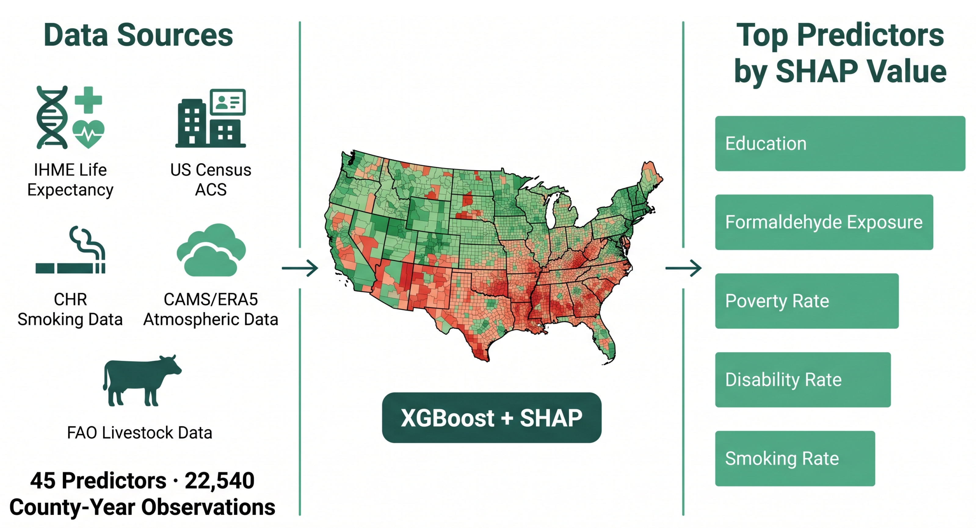
Drawing on the external exposome framework, the totality of environmental exposures encountered throughout a lifetime [21], we develop an interpretable machine learning framework to model county-level life expectancy across the United States using an integrated dataset spanning socioeconomic conditions, smoking prevalence, atmospheric exposures, and livestock density. The overall workflow is summarized in Figure 2. We use data from the Institute for Health Metrics and Evaluation (IHME), the American Community Survey (ACS), County Health Rankings, the Copernicus Atmosphere Monitoring Service (CAMS), ERA5, and livestock distribution datasets for the period 2012–2019 [18,22,23,24,25]. Our modeling approach employs XGBoost, a gradient boosting algorithm known for its ability to capture complex non-linear relationships and interactions among high-dimensional features [26], and utilizes SHAP values and permutation importance to identify the most influential predictors. Our analysis shows that while traditional socioeconomic variables remain strong predictors, atmospheric variables such as formaldehyde exposure and wet-bulb temperature also provide important predictive information for county-level life expectancy.

2. Methodology

This study integrates county-level data from five primary sources to model life expectancy across the contiguous United States from 2012 to 2019. Life expectancy estimates were obtained from the Institute for Health Metrics and Evaluation (IHME) [22], while socioeconomic variables were drawn from the American Community Survey (ACS) 5-year estimates [23]. County-level smoking prevalence was obtained from County Health Rankings analytic data releases [24]. Atmospheric data, including pollutant concentrations and meteorological variables, were sourced from the Copernicus Atmosphere Monitoring Service (CAMS) and the European Centre for Medium-Range Weather Forecasts ERA5 reanalysis [25]. Livestock density data were obtained from Gilbert et al. [18]. Each of these datasets was preprocessed and combined, and the final integrated dataset was used to train an XGBoost model [26]. Model performance was evaluated using R², adjusted R², root mean square error (RMSE), and mean absolute error (MAE), while feature importance was assessed through SHAP values and permutation importance. A brief description of the datasets that were used in this analysis is included below:

2.1. IHME Dataset

Life expectancy estimates were obtained from the Institute for Health Metrics and Evaluation (IHME), which provides annual county-level estimates of mean life expectancy at birth across the United States from 2000 to 2019 [22]. These estimates are derived from population and mortality data provided by the National Center for Health Statistics and represent stratified estimates by age group, race, and ethnicity [1]. For this study, we used life expectancy at birth estimates for the total population, which includes all racial and ethnic groups. In the IHME dataset, this metric is indexed under the age group “under 1 year of age,” but it refers to the standard demographic measure of life expectancy at birth derived from age-specific mortality rates across the full population. It is not restricted to infant or perinatal deaths. The IHME dataset covers all counties in the contiguous United States, enabling a comprehensive analysis of life expectancy disparities. Data from 2012 to 2019 were selected to align with the temporal coverage of the atmospheric and socioeconomic datasets.

2.2. ACS Dataset

Socioeconomic and demographic variables were obtained from the American Community Survey (ACS) 5-year estimates for 2012 to 2019 [23]. The 5-year estimates were selected over the 1-year estimates due to their greater statistical reliability for small geographic units such as counties, which is essential for county-level spatial modeling [27]. The 1-year estimates, while temporally more precise, only cover counties with populations of 65,000 or more and would have limited our analysis to non-rural areas [28].

We initially retrieved approximately 20 variables from the ACS using the U.S. Census Bureau API, including poverty rate, median household income, unemployment rate, educational attainment (percentage with a bachelor’s degree or higher), and racial composition. Racial composition was calculated as the proportion of each racial/ethnic group relative to the total county population. After removing highly correlated and redundant features during preprocessing, 10 variables were retained for the final model. These socioeconomic indicators were selected based on prior research linking income, education, and demographic structure to mortality and health outcomes [4,5]. The final retained variables are listed in Appendix A.

2.3. County Health Rankings Smoking Dataset

County-level adult smoking prevalence was obtained from the official County Health Rankings analytic data releases for 2012 through 2019 [24]. Each yearly file provided a county FIPS code and an adult smoking estimate. State summary rows and the national aggregate row were removed, county FIPS codes were standardized to five digits, and the yearly files were combined into a common county-year table. The smoking values were already reported on a 0–1 scale, so no additional rescaling was needed.

The County Health Rankings methodology changed during the study period. The earlier releases were based on multi-year BRFSS aggregation, whereas the later releases used modeled county estimates. This change affected both county coverage and year-to-year variation, with broader coverage after 2015. To account for that shift, we added a binary post-2015 indicator coded 0 for 2012–2015 and 1 for 2016–2019. This indicator was included during model fitting as a measurement-control variable and was not interpreted as a scientific predictor.

2.4. CAMS Dataset

Atmospheric and meteorological variables were obtained from the Copernicus Atmosphere Monitoring Service (CAMS) global reanalysis (EAC4) and the European Centre for Medium-Range Weather Forecasts (ECMWF) ERA5 reanalysis [25]. CAMS assimilates satellite observations including OMI for tropospheric composition, MODIS for aerosol optical depth, and GOME-2 for trace gases, combining remote sensing data with atmospheric modeling to provide spatially continuous estimates [25]. The CAMS EAC4 dataset provides gridded atmospheric composition data at 0.75° × 0.75° spatial resolution with 3-hourly temporal resolution, including air pollutants (PM_2.5, O₃, NO₂, formaldehyde) at both surface level and total column, along with meteorological variables. ERA5 provided relative humidity data at 0.25° × 0.25° resolution. The CAMS EAC4 and ERA5 datasets were each processed independently at their native resolutions (0.75° × 0.75° and 0.25° × 0.25°, respectively). Each was spatially interpolated to county boundary points using multilinear interpolation, with no intermediate regridding to a common spatial grid. The interpolated values were then averaged across boundary points for each county. Temporal aggregation was performed by calculating annual averages from the 3-hourly observations (approximately 2960 time points per year). At the end, we had approximately 60 atmospheric features for 2012–2019, including pollutant concentrations, temperature, humidity, and wind velocity. Several atmospheric variables were derived as fraction-of-time (FoT) metrics, which capture the frequency of elevated pollutant exposure over the course of a year. The FoT computation follows a three-step procedure. First, for each calendar year, the annual county-level average of each pollutant variable was computed for all approximately 3100 counties in the contiguous United States. Second, the 75th percentile of these annual averages was computed across all counties for that year, yielding a year-specific national reference threshold. Third, for each county, the FoT value was calculated as the proportion of three-hourly CAMS timestamps in that year during which the county-level CAMS-derived concentration exceeded this threshold. For example, FoT Formaldehyde Above 75th Percentile represents the fraction of three-hourly measurements in a given year during which a county’s formaldehyde concentration exceeded the 75th percentile of annual county averages for that year, computed across all counties in the contiguous United States. This threshold is derived independently for each calendar year and reflects a national atmospheric reference level, not estimated from the train/test partition used for machine learning. A complete list of atmospheric variables is provided in Appendix A.

2.5. Livestock Data

Livestock density data were obtained from the Food and Agriculture Organization (FAO) Gridded Livestock of the World (GLW) dataset, which provides species-specific density estimates (heads/km²) at approximately 10 km resolution for seven species: cattle, chicken, duck, goat, horse, pig, and sheep [18,29]. The gridded raster data were aggregated to county-level boundaries using area-weighted zonal statistics, with densities calculated only for agricultural land identified from the 2019 National Land Cover Database. Because GLW data were available only for discrete years (2010, 2015, 2020), annual values for 2012–2019 were generated through linear interpolation between these time points. This yielded seven livestock density features for each county–year observation, serving as proxies for agricultural intensity and associated emissions such as ammonia (${\mathrm{NH}}_3$), methane (${\mathrm{CH}}_4$), and nitrous oxide (${\mathrm{N}}_2\mathrm{O}$) [19]. The full set of data sources is summarized in

Table 1. Summary of data sources used in this study.

Source	Description	Period	Resolution	N
IHME	Life expectancy at birth	2012–2019	County-level	Target
ACS 5-year	Socioeconomic and demographic indicators	2012–2019	County-level	10
County Health Rankings	Adult smoking rate and post-2015 methodology indicator	2012–2019	County-level	2
CAMS/ERA5	Atmospheric pollutants and meteorological variables	2012–2019	County-level (from 0.75°/0.25° grids)	26
FAO GLW	Livestock density by species	2012–2019 (interpolated)	County-level (from ∼10 km grids)	7
Total predictor features: 45

.

2.6. Data Processing

The life expectancy, ACS, CAMS/ERA5, and livestock datasets were first merged by county FIPS codes and year to create an integrated county-year panel. Missing values, denoted either as NaN or as the sentinel value −666,666,666, were handled through listwise deletion to avoid introducing imputation bias and maintain internal consistency across features. To reduce multicollinearity among atmospheric variables, features with pairwise correlations exceeding 0.85 were identified through hierarchical clustering analysis, and the most interpretable feature from each correlated cluster was retained for modeling. County-level smoking prevalence and the post-2015 methodology indicator were then merged by county FIPS code and year. The pre-smoking integrated dataset contained 24,487 county-year observations. Of these, 1947 observations (7.95%) lacked smoking data and were excluded from the final complete-case analysis. The final modeling dataset therefore comprised 22,540 county-year observations from 3061 counties spanning 2012–2019, with 45 predictor variables and 1 target variable (life expectancy). Metadata columns such as County, State, Year, and FIPS codes were retained for identification purposes but excluded from the feature matrix used for modeling. Because the datasets for 2012–2019 were stacked vertically and the same counties are repeated across multiple years, standard random splitting would have allowed observations from the same county to appear in both training and test sets, leading to data leakage and inflated performance metrics. To prevent this, we employed GroupShuffleSplit with county FIPS codes as the grouping variable, ensuring that all observations from a given county were assigned exclusively to either the training set (80%) or the test set (20%). This forces the model to predict the life expectancy of counties that it did not see during training.

2.7. Modeling Approach

The preprocessed 45-predictor dataset was used to train an XGBoost gradient boosting regressor, selected for its ability to capture complex non-linear relationships and feature interactions while incorporating L1 and L2 regularization to prevent overfitting [26]. Hyperparameter optimization was performed using Bayesian optimization via BayesSearchCV, which efficiently explores the hyperparameter space through probabilistic modeling rather than exhaustive grid search [30]. The search space included n_estimators (200–1500), max_depth (4–8), learning_rate (0.01–0.15), subsample (0.6–0.95), colsample_bytree (0.5–0.9), L1 regularization (reg_alpha, 0.01–5.0), L2 regularization (reg_lambda, 0.1–5.0), and min_child_weight (3–15). Bayesian optimization was configured with 50 iterations and 5-fold GroupKFold cross-validation, using R² as the optimization metric. GroupKFold ensures that during each cross-validation fold, all observations from a given county remain together, preventing the same county from appearing in both the training and validation portions of any fold. The final 80/20 grouped split produced 18,028 training observations from 2448 counties and 4512 test observations from 613 counties, with no county overlap between the two partitions. The best-performing hyperparameter configuration, reported in

Table 2. Optimal hyperparameters obtained through Bayesian optimization for the full 45-feature model.

Parameter	Optimal Value
n_estimators	1500
max_depth	8
learning_rate	0.010
subsample	0.748
colsample_bytree	0.50
reg_alpha	0.533
reg_lambda	5.00
min_child_weight	15

, was selected and used to train the final model on the entire training set. The same optimization procedure was applied to reduced feature sets in the ablation analysis.

Model performance was evaluated using R², adjusted R², root mean squared error (RMSE), and mean absolute error (MAE). RMSE and MAE were selected because both are expressed in the same units as the target variable (years), providing intuitive measures of prediction error. Adjusted R² was used to assess the proportion of variance explained by the model while penalizing model complexity, making it particularly suitable for high-dimensional datasets where standard R² can be inflated by the inclusion of numerous predictors. All metrics were computed separately on training and test sets to evaluate model generalization and detect potential overfitting.

2.8. Modeling Interpretability

To interpret the trained XGBoost model and identify the most influential predictors of life expectancy, we employed two complementary feature importance methods. Permutation importance was calculated by randomly shuffling each feature’s values in the test set and measuring the resulting degradation in model performance (RMSE), with greater performance drops indicating higher feature importance. SHAP (SHapley Additive exPlanations) values were computed using the TreeExplainer algorithm to quantify each feature’s contribution to individual predictions, providing both global importance rankings and directional effects [31]. Unlike permutation importance, SHAP values are grounded in cooperative game theory and account for feature interactions, offering more robust interpretability for correlated predictors [31]. SHAP dependence plots were generated for the leading predictors to examine how feature values were related to their model contributions. The post-2015 County Health Rankings indicator was included during model fitting as a measurement-control variable but was excluded from interpretation plots and substantive feature rankings because it reflects a change in smoking-data measurement rather than a life-expectancy exposure. To assess feature redundancy, we conducted an ablation study by systematically retraining the model with progressively reduced feature sets based on the revised SHAP rankings (top 20, top 10, and top 5 features), evaluating the tradeoff between model complexity and predictive performance. Model calibration and prediction errors were assessed through residual analysis, examining the distribution and patterns of residuals (observed minus predicted values) across the range of predicted life expectancy values.

2.9. Robustness and Diagnostic Methods

Several diagnostic and sensitivity analyses were conducted to assess whether the main findings held under different conditions. These tests examined potential confounding by poverty, education, and smoking, generalization across time, geographic clustering of prediction errors, stability of feature rankings, and the effect of selected modeling choices.

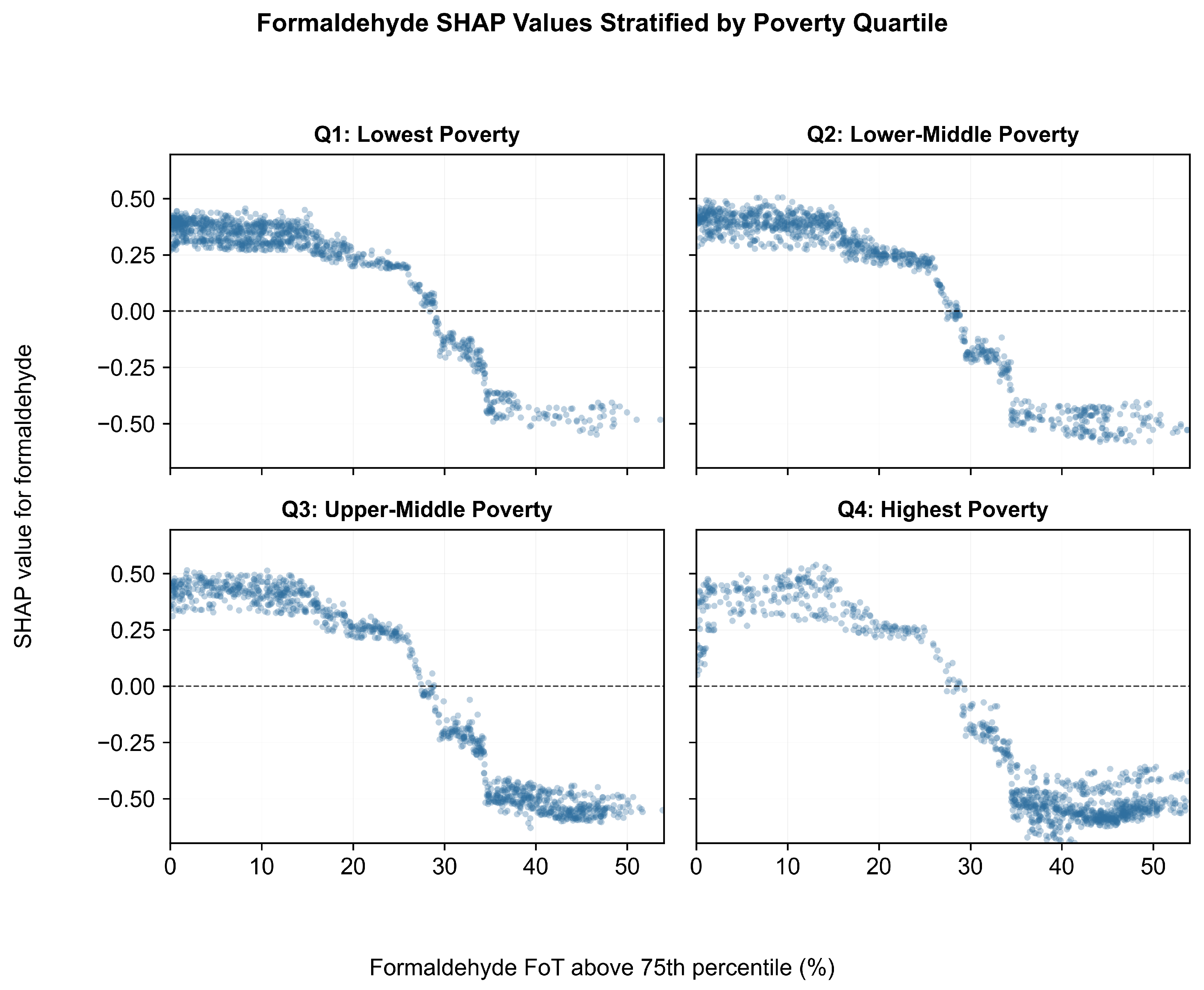
Socioeconomic confounding assessment. A concern with any atmospheric predictor is that counties with high pollution may also tend to be poorer or have higher smoking rates. If so, the model could be using the atmospheric variable partly as a proxy for social conditions. To address this, we divided the held-out test observations into poverty-rate quartiles and examined the relationship between formaldehyde exposure and formaldehyde SHAP values within each quartile. We also computed a partial correlation between formaldehyde exposure and life expectancy. This test measures the formaldehyde-life expectancy association after accounting for poverty rate, educational attainment, and smoking rate. It asks whether formaldehyde carries predictive information beyond what poverty, education, and smoking rates can explain on their own.

Temporal validation. The main validation split tests whether the model predicts life expectancy in counties it has never seen. A separate question is whether the same relationships hold when applied to later years of data. To test this, we trained the model on observations from 2012–2016 and evaluated it on observations from 2017–2019, using the same hyperparameters from the full model. This temporal test evaluates whether the associations between predictors and life expectancy remained stable across the study period.

Spatial autocorrelation of residuals. Prediction errors can be randomly scattered, or they can cluster geographically, with neighboring counties being consistently overpredicted or underpredicted. We tested for this pattern using Moran’s I, a standard spatial statistic that measures whether nearby locations have more similar values than expected by chance [32]. Residuals from the held-out test set were first averaged within each county across years, so that each test county contributed one mean prediction error. Geographic neighbors were then defined using a k-nearest-neighbor spatial weights matrix with k = 8, based on county centroid locations. Moran’s I was computed using these weights and the county-level mean residuals.

SHAP ranking stability. A feature importance ranking from a single split may depend on which counties happened to fall in the training or test set. To test whether the formaldehyde ranking was stable, we repeated the SHAP analysis across five county-grouped folds. In each repetition, one group of counties was held out for evaluation while the remaining counties were used for training. All observations from the same county were kept together, so no county appeared in both the training and evaluation sets within a fold. The same hyperparameters from the full model were used throughout, and the rank of formaldehyde was recorded in each fold.

CAMS resolution diagnostic. The CAMS EAC4 atmospheric data are provided at a grid resolution of 0.75° × 0.75°, so a single atmospheric grid cell can cover multiple counties. To quantify this, we counted how many county centroids fell within each approximate 0.75° × 0.75° support region. This count was computed for all study counties and for the held-out test counties. It is an approximate diagnostic rather than a reconstruction of the original interpolation pipeline, but it shows how often counties fall within the same coarse atmospheric grid region.

Livestock sensitivity analysis. Livestock density values for years between 2010, 2015, and 2020 were estimated by linear interpolation. To test whether these approximate values affected the main findings, we repeated the analysis after removing all seven livestock predictors. The same training–test split and hyperparameters were used, and model performance and formaldehyde ranking were compared with the full model.

Bayesian optimization convergence. To evaluate whether the hyperparameter search was run for a sufficient number of iterations, we tracked the best cross-validated R² score found at each step of the 50-iteration search. If the best score stopped improving well before the final iteration, it indicated that additional iterations were unlikely to change the selected hyperparameters.

3. Results

3.1. Model Performance

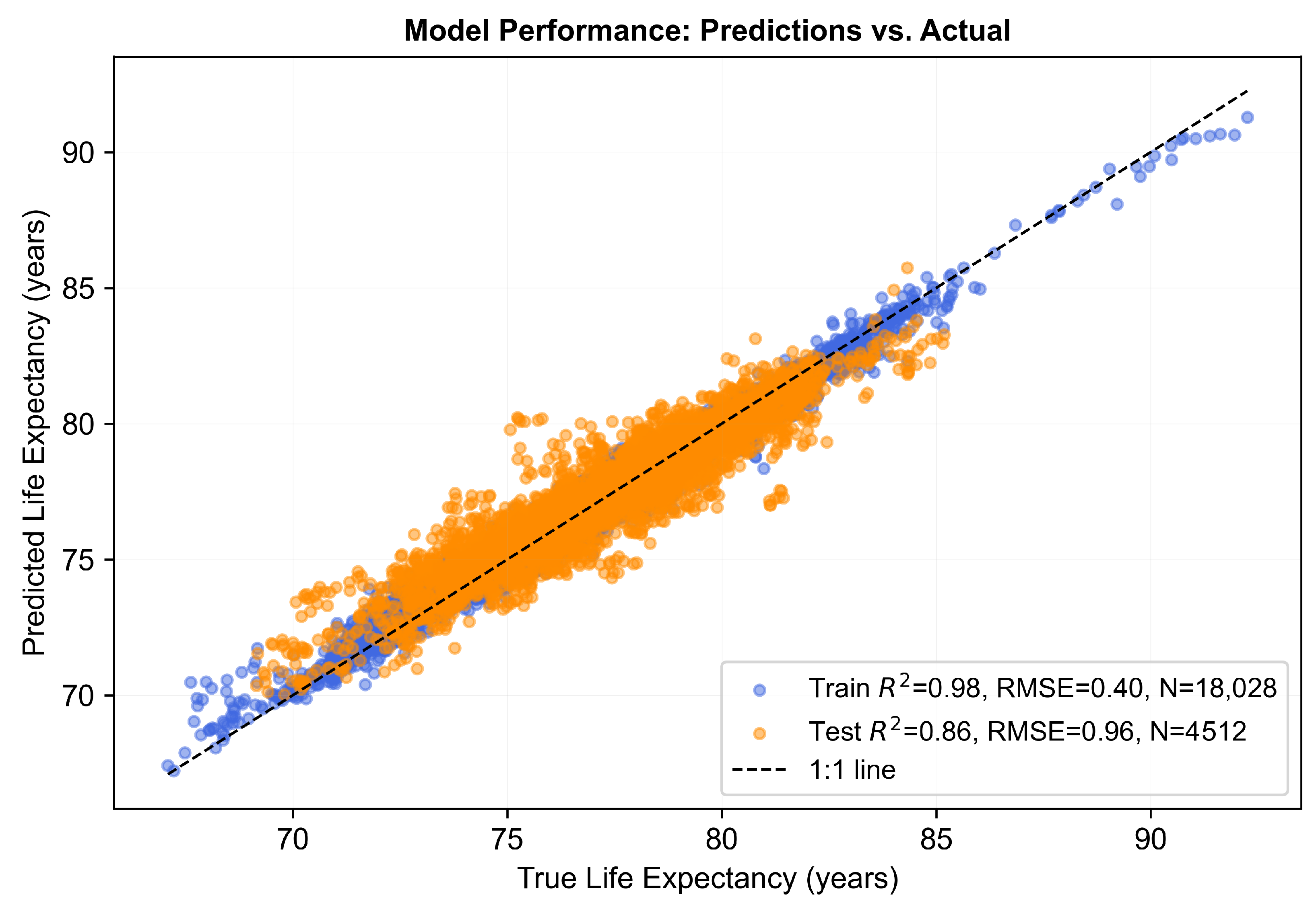
The XGBoost model trained on all 45 predictors achieved strong held-out performance (Figure 3), with a test R² of 0.863, adjusted R² of 0.861, RMSE of 0.96 years, and MAE of 0.72 years across 4512 test observations. Training performance was higher, with R² = 0.975, RMSE = 0.40 years, and MAE = 0.31 years across 18,028 training observations. The train–test split contained 2448 training counties and 613 test counties, with no county overlap between the two groups. This grouped design reduces leakage from repeated county-year observations and evaluates whether the model can predict life expectancy in counties that were not used during training.

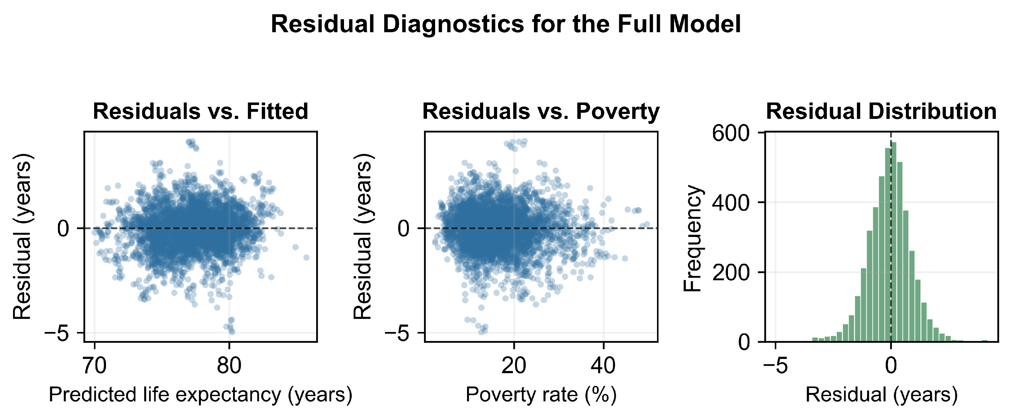
Residual diagnostics are shown in Figure 4. Residuals were centered near zero and showed no strong systematic pattern across the fitted values. The residuals also showed no clear monotonic trend with poverty rate, suggesting that prediction errors were not dominated by this leading socioeconomic predictor.

3.2. Feature Importance Analysis

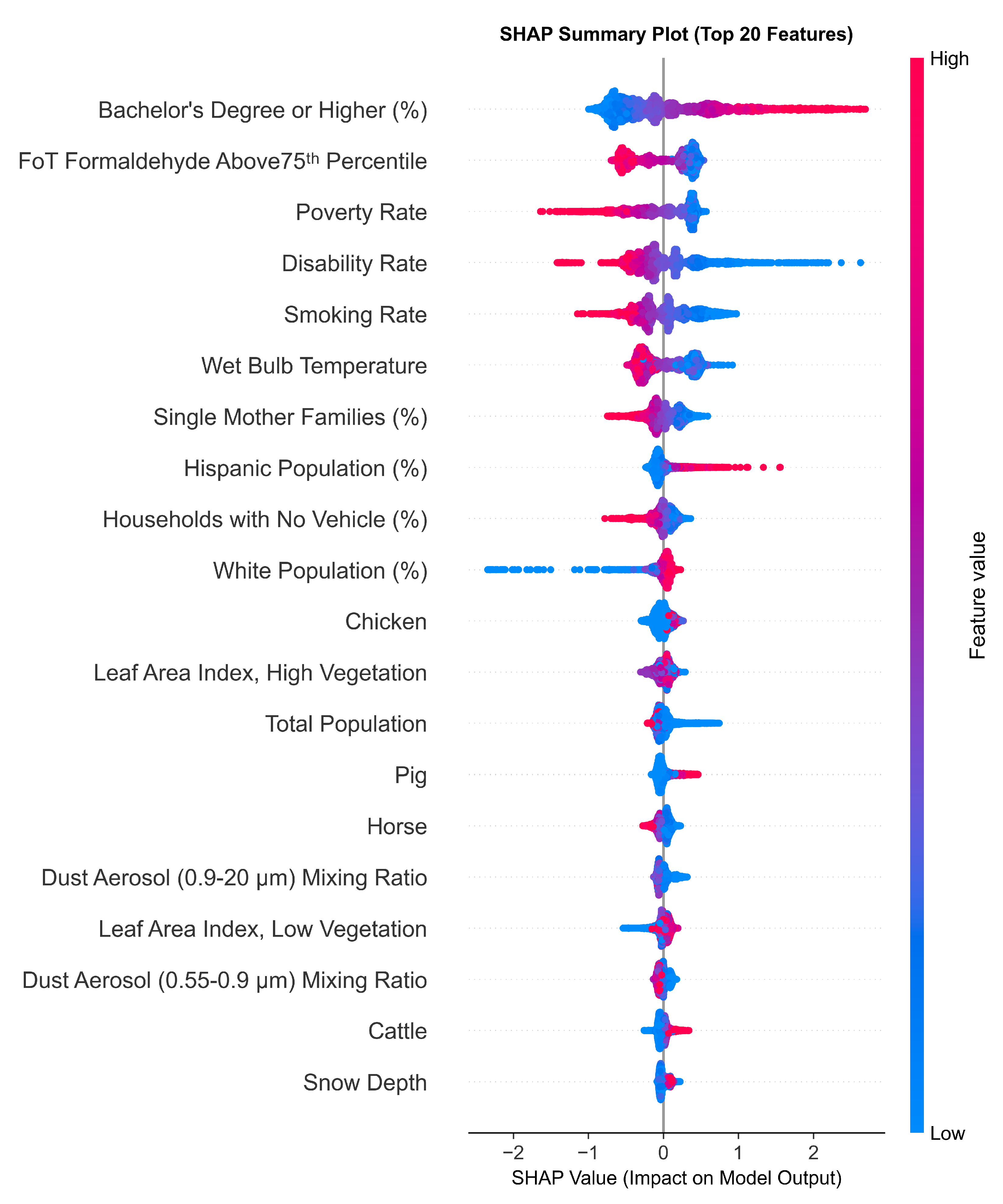
SHAP analysis of the full 45-predictor model identified educational attainment (Bachelor’s Degree or Higher) as the most important predictor, followed by FoT Formaldehyde Above 75th Percentile, poverty rate, disability rate, smoking rate, and wet-bulb temperature (Figure 5). The mean absolute SHAP values for these six predictors were 0.579, 0.381, 0.345, 0.340, 0.306, and 0.284, respectively. Formaldehyde exposure therefore ranked second overall and remained the highest-ranked atmospheric pollutant in the model.

Smoking Rate was included directly in the full model and ranked fifth, with a mean absolute SHAP value of 0.306. Formaldehyde ranked second, with a mean absolute SHAP value of 0.381, after accounting for county-level smoking prevalence. This indicates that formaldehyde retained substantial predictive importance when smoking was included in the feature set.

Socioeconomic predictors were prominent in the importance rankings. The beeswarm plot (Figure 5) showed that counties with higher educational attainment tended to have higher predicted life expectancy, while counties with higher poverty, disability, and smoking rates tended to have lower predicted life expectancy. These patterns align with established literature linking socioeconomic disadvantage to adverse health outcomes [4,5].

Atmospheric and environmental variables also appeared among the leading predictors. Higher formaldehyde exposure was concentrated on the negative side of the SHAP plot, indicating lower predicted life expectancy in counties where formaldehyde exceeded the 75th percentile more often. Wet-bulb temperature ranked sixth and also showed predominantly negative SHAP values at higher levels, consistent with the health burden of heat and humidity. Additional atmospheric variables in the top 20 included leaf area indices for high and low vegetation, two dust aerosol size fractions, and snow depth. Livestock density variables appeared among secondary predictors, with chicken, pig, horse, and cattle density all ranking within the top 20.

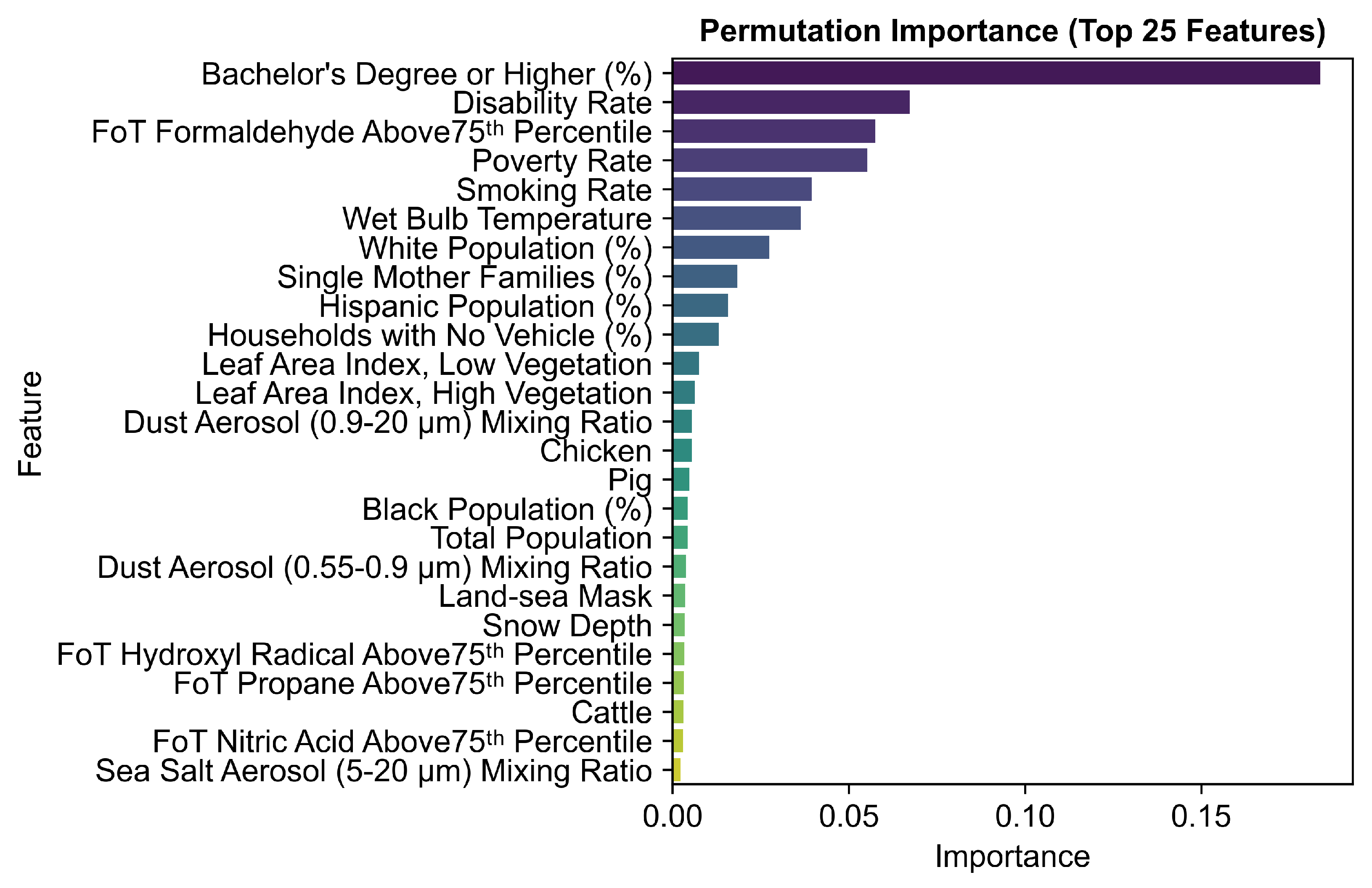
Permutation importance provided a second test of feature importance by measuring how much model performance declined when each predictor was shuffled. This analysis also ranked education first and placed formaldehyde among the leading predictors, behind disability rate and ahead of poverty rate, smoking rate, and wet-bulb temperature (Figure 6). The broadly consistent rankings from SHAP and permutation importance support the conclusion that formaldehyde provided meaningful predictive information in the full model.

3.3. Feature Ablation Study

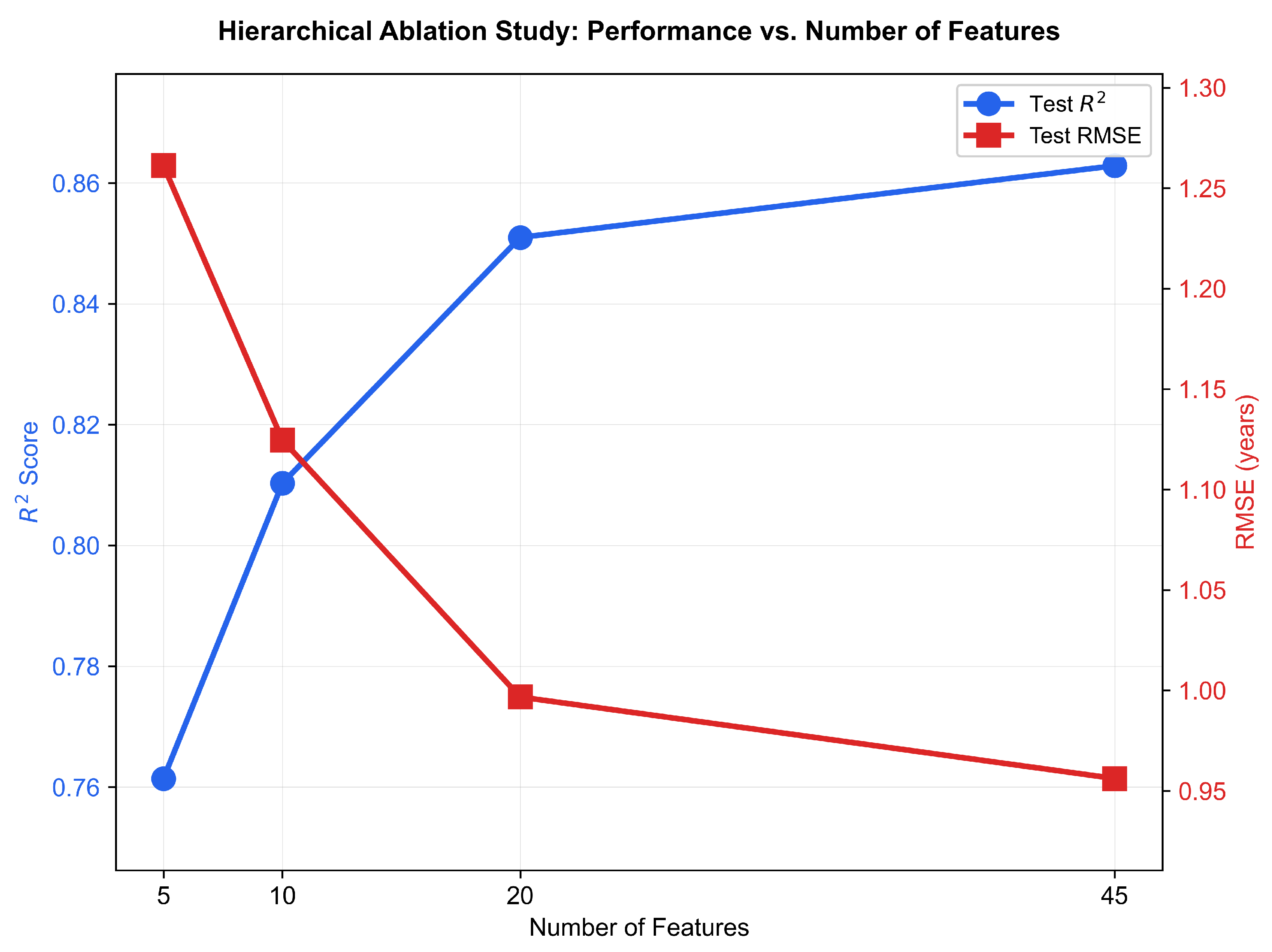
To examine how many predictors were needed to preserve model performance, we retrained the XGBoost model using progressively smaller feature sets. The top 20 predictors were selected from the SHAP ranking of the full 45-predictor model. The top 10 predictors were then selected from the top 20 model, and the top 5 predictors were selected from the top 10 model. Hyperparameters were re-optimized for each reduced model using Bayesian optimization. Performance metrics across all models are shown in

Table 3. Model performance metrics across the feature ablation study. The top 20 model retained performance close to the full 45-predictor model.

Feature Set	N Features	Train R2	Test R2	Train RMSE	Test RMSE	Test MAE
All Features	45	0.975	0.863	0.40	0.96	0.72
Top 20	20	0.970	0.851	0.45	1.00	0.75
Top 10	10	0.948	0.810	0.59	1.12	0.85
Top 5	5	0.834	0.761	1.04	1.26	0.96

and Figure 7.

The top 20 model achieved strong performance, with a test R² of 0.851, RMSE of 1.00 years, and MAE of 0.75 years. This was only slightly below the full model, which achieved a test R² of 0.863, RMSE of 0.96 years, and MAE of 0.72 years. Performance declined more clearly in the top 10 model (R² = 0.810, RMSE = 1.12 years, MAE = 0.85 years) and the top 5 model (R² = 0.761, RMSE = 1.26 years, MAE = 0.96 years). This pattern suggests that many lower-ranked predictors were partly redundant, but that reducing the model below 20 predictors removed important information.

Feature rankings were also stable across reduced models. Educational attainment remained the top predictor, and formaldehyde remained among the leading predictors as the feature set was reduced. In the full model, formaldehyde ranked second by SHAP importance. Its continued prominence in reduced models supports the finding that formaldehyde provided predictive information that was not limited to the lowest-ranked features.

3.4. Robustness and Diagnostic Analyses

The formaldehyde result remained after accounting for major socioeconomic predictors and smoking prevalence. In the held-out test set, formaldehyde SHAP values showed a similar non-linear pattern within each poverty quartile (Figure 8). Formaldehyde also remained negatively associated with life expectancy after accounting for poverty rate, educational attainment, and smoking rate. The partial correlation was −0.419 across county-year observations ($p<{10}^{-190}$, N = 4512) and −0.399 after averaging to the county level ($p<{10}^{-24}$, N = 613). These results indicate that formaldehyde retained predictive information beyond what poverty, education, and smoking rates explained.

The model also generalized well across time. When trained on observations from 2012–2016 and tested on observations from 2017–2019, it achieved a test R² of 0.886, RMSE of 0.89 years, and MAE of 0.67 years. This temporal result suggests that the relationships learned from earlier years remained useful for predicting later years in the study period.

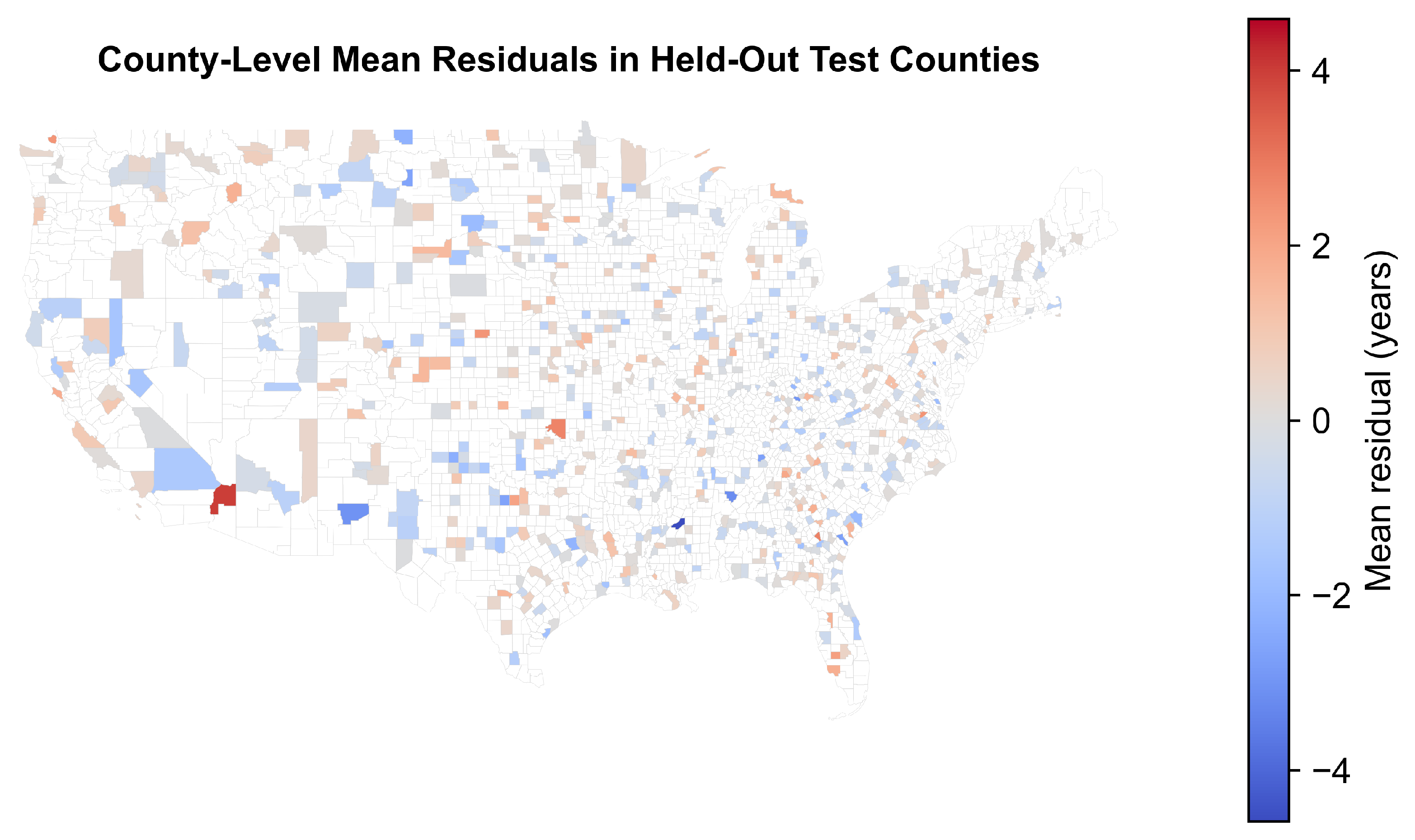
Residuals showed weak but statistically significant spatial clustering, with the spatial distribution of county-level mean residuals shown in Figure 9. Moran’s I for county-level mean residuals was 0.059 (p = 0.0016, N = 613), using 8-nearest-neighbor spatial weights. This value is close to zero, indicating that prediction errors were not fully independent in space, although the magnitude of clustering was small.

The SHAP ranking was stable across validation folds. In five GroupKFold repetitions, formaldehyde ranked second in every held-out fold. This indicates that the formaldehyde ranking was not driven by a single favorable train–test split.

The CAMS resolution diagnostic showed that multiple counties can share the same approximate atmospheric grid cell. Across all study counties, each approximate 0.75° × 0.75° grid cell contained a mean of 2.56 counties, a median of 2 counties, and a maximum of 11 counties. Among held-out test counties, the mean was 1.26 counties per grid cell, the median was 1, and the maximum was 4. This confirms that the CAMS grid is coarse relative to some county boundaries, while also showing that most held-out test grid cells contained only one test county.

Removing livestock predictors did not materially change the main findings. After all seven livestock variables were removed, test R² changed from 0.863 to 0.861, RMSE changed from 0.956 to 0.964 years, and MAE changed from 0.719 to 0.729 years. Formaldehyde remained ranked second. This indicates that the main formaldehyde result was not dependent on interpolated livestock density variables.

Finally, the Bayesian optimization search showed early stabilization. Across the 50-iteration search, the final best cross-validated R² was 0.845. The best score was already within 0.001 of this value by iteration 5 and within 0.0005 by iteration 19. This convergence pattern suggests that the selected hyperparameters were not an artifact of stopping the search too early.

4. Discussion

4.1. Formaldehyde: An Underappreciated Environmental Predictor

The emergence of formaldehyde exposure as the second-ranked predictor of life expectancy is a notable finding. Formaldehyde is a ubiquitous volatile organic compound (VOC) with indoor sources, including building materials, pressed wood products, household furniture, and combustion appliances, as well as outdoor sources, including vehicle emissions, industrial processes, and photochemical reactions in the atmosphere [33,34]. Despite widespread population exposure, formaldehyde has received less attention in life expectancy modeling than more commonly studied air pollutants such as fine particulate matter (PM_2.5) and ozone.

The result is also somewhat unexpected. Formaldehyde is short-lived in the atmosphere, and its strongest cancer evidence has historically focused on relatively specific outcomes such as nasopharyngeal cancer and leukemia [35]. However, recent evidence also links ambient formaldehyde with non-accidental, circulatory, and respiratory mortality [36], and mechanistic studies connect formaldehyde exposure to cardiovascular injury, oxidative stress, systemic inflammation, DNA damage, and immunological dysregulation [37,38,39]. These mechanisms make the predictive association biologically plausible, even though the present study cannot establish causality.

The robustness analyses strengthen confidence in this association. Formaldehyde ranked second and smoking rate ranked fifth in the full 45-predictor model. The poverty-stratified SHAP analysis (Figure 8) and partial correlation analysis also showed that the formaldehyde-life expectancy association persisted after accounting for poverty rate, educational attainment, and smoking rate. These findings do not establish causality, but they suggest that the formaldehyde signal was not solely a proxy for socioeconomic disadvantage or county-level smoking prevalence.

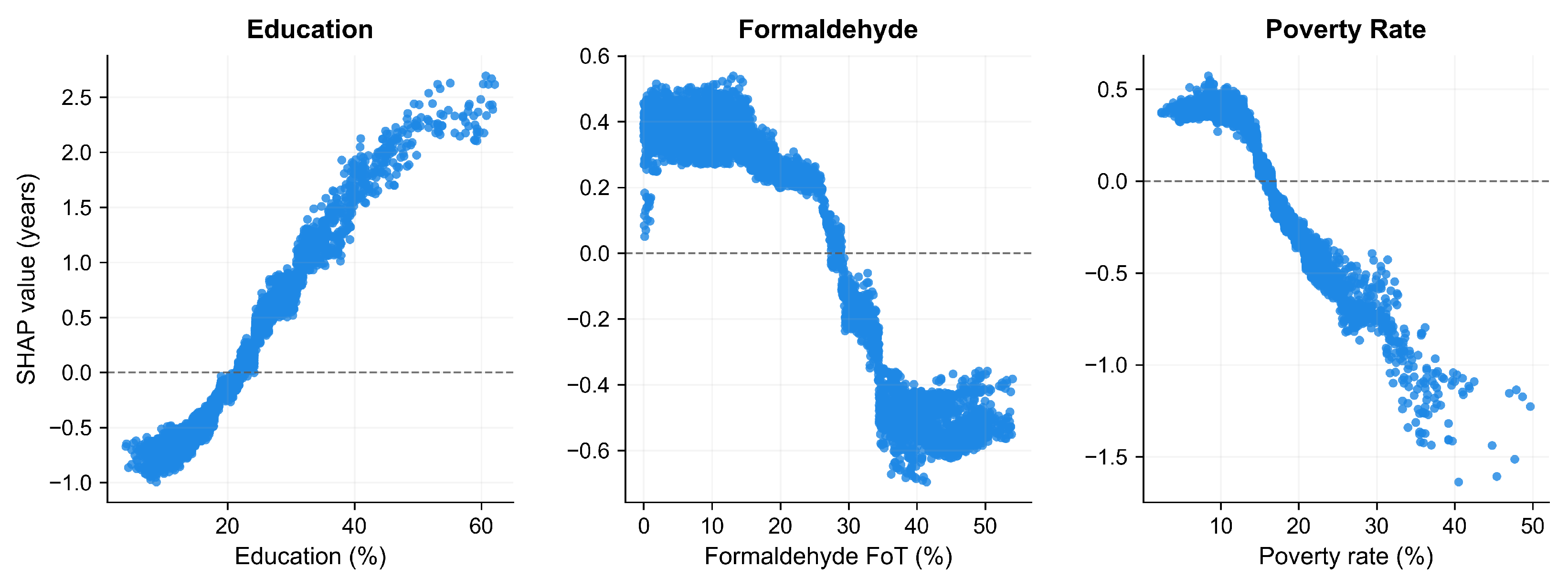
The SHAP dependence plot (Figure 10) further shows a non-linear pattern. The model predicts lower life expectancy most clearly when formaldehyde exceeds the 75th percentile more than approximately 30% of the time. This pattern should be interpreted cautiously, but it suggests that frequent formaldehyde exceedances may be more informative than occasional exceedances.

Current air quality monitoring prioritizes criteria pollutants, including ozone, particulate matter, carbon monoxide, sulfur dioxide, nitrogen dioxide, and lead. Formaldehyde remains less routinely monitored [40], despite classification as a Hazardous Air Pollutant under Section 112 of the U.S. Clean Air Act [41]. Ground-level formaldehyde observations are sparse [42], which limits direct assessment of population exposure. Satellite remote sensing can help fill this gap, with instruments such as OMI and TROPOMI providing spatially continuous formaldehyde observations that complement ground-based networks [43]. The prominence of formaldehyde in this analysis therefore supports further epidemiological research using finer exposure assessment, independent satellite validation, and causal inference designs to test whether this predictive association reflects an underlying health pathway.

4.2. Socioeconomic and Environmental Predictors

Educational attainment emerged as the strongest predictor in the full 45-predictor model, confirming extensive literature on the role of social determinants in health outcomes [4,44]. Poverty rate, disability rate, and smoking rate also ranked among the leading predictors. Counties with higher educational attainment tended to have higher predicted life expectancy, while counties with higher poverty, disability, and smoking rates tended to have lower predicted life expectancy. These patterns are expected and support the validity of the model because they align with well-established population health gradients [4,5,10].

Wet-bulb temperature ranked sixth, making it one of the leading environmental predictors. Unlike dry-bulb temperature, wet-bulb temperature combines heat and humidity, making it a physiologically relevant measure of heat stress and the body’s ability to cool itself through evaporation [45]. Very high wet-bulb temperatures can impair thermoregulation, and a wet-bulb temperature near 35°C is often described as an approximate upper limit for sustained human survival [46,47]. Studies have also linked extreme heat and non-optimal temperatures with increased mortality [48,49]. The prominence of wet-bulb temperature in the model is therefore consistent with evidence that combined heat and humidity provide predictive information about heat-related health stress.

Some SHAP patterns require careful interpretation. Hispanic Population (%) showed a positive association with predicted life expectancy. This pattern may be consistent with the Hispanic mortality paradox, in which Hispanic populations in the United States often show lower mortality than expected despite socioeconomic disadvantage [50]. It should not be interpreted as evidence that ethnicity itself explains longer life expectancy. At the county level, this variable may also capture age structure, migration patterns, social networks, geography, or other factors not fully measured in the model.

The livestock and vegetation variables should be interpreted with similar caution. Livestock density variables are broad proxies for agricultural intensity and rural land use, not direct measures of individual exposure. Differences in SHAP direction across animal types may reflect regional agricultural systems, rurality, economic structure, or other county characteristics rather than animal-specific health effects. Likewise, the leaf area index variables do not directly measure individual access to green space. Although prior studies have linked green space with lower mortality [51], the CAMS vegetation variables reflect grid-level land surface characteristics. Their SHAP patterns may therefore capture land use, climate, agriculture, and rural-urban gradients rather than a simple protective or harmful effect of vegetation itself.

4.3. Limitations and Future Directions

This study has several limitations. First, the analysis is observational. It identifies predictive associations between county-level exposures and life expectancy, but it cannot establish causality. County-level aggregation also introduces ecological fallacy risk because population-level associations may not reflect individual-level relationships. Future work should therefore use individual-level exposure and outcome data, causal inference methods, and mechanistic studies to test whether the predictive association observed here reflects individual-level exposure-response relationships.

Second, the model now includes county-level smoking prevalence, but it does not include all behavioral and clinical risk factors that influence life expectancy. Obesity, physical inactivity, diet, healthcare access, and occupational exposures were not directly measured. Some of these factors are socially patterned and may overlap with education, poverty, and smoking [10], but they are not fully captured by those variables. Residual confounding therefore remains possible.

Third, atmospheric exposures were derived from CAMS/ERA5 reanalysis products rather than dense ground-based monitoring networks. The 0.75° × 0.75° CAMS resolution is coarse relative to many counties, especially in the eastern United States. This can smooth local exposure gradients and can cause nearby counties to share similar atmospheric information. Our grid-support diagnostic quantified this issue, but it does not remove the underlying exposure uncertainty. Future work should compare CAMS-derived formaldehyde estimates with independent satellite retrievals, especially TROPOMI, and with ground-based measurements where available [42,43]. The CAMS EAC4 reanalysis also does not provide benzene, toluene, or other BTEX compounds. Future analyses using ground-based monitoring networks or higher-resolution chemical transport models could add these compounds.

Fourth, residuals showed weak but statistically significant spatial autocorrelation. This indicates that prediction errors were not fully independent in space, even though the magnitude of clustering was small. Future work could evaluate spatial cross-validation, spatially explicit models, or region-stratified analyses to test whether the same predictors remain important under stricter spatial assumptions.

Finally, livestock density data from the FAO Gridded Livestock of the World dataset were available only for 2010, 2015, and 2020. Annual values for 2012–2019 were generated through linear interpolation between these anchor years. This assumes that livestock populations changed smoothly between observed years, which may not hold in every county. The livestock sensitivity analysis showed that removing all livestock predictors had little effect on model performance and did not change the formaldehyde ranking, but livestock variables should still be interpreted as approximate annual estimates. The analysis is also limited to US counties from 2012–2019, so generalization to other countries or time periods remains untested.

5. Conclusions

This study demonstrates that an external exposome approach integrating atmospheric exposures, socioeconomic conditions, livestock density, and smoking prevalence with machine learning can identify important predictors of county-level life expectancy. In the final 45-predictor model, formaldehyde ranked second overall after accounting for smoking prevalence, poverty, and educational attainment. Wet-bulb temperature also emerged as a leading environmental predictor, suggesting that atmospheric exposures and heat-humidity stress provide predictive information beyond traditional socioeconomic variables. Because these findings are observational and county-level, future research should use finer exposure data, individual-level outcomes, and causal inference designs to test the associations suggested by this analysis.

References

1. Dwyer-Lindgren, L.; Bertozzi-Villa, A.; Stubbs, R.W.; Morozoff, C.; Mackenbach, J.P.; van Lenthe, F.J.; Mokdad, A.H.; Murray, C.J.L. Inequalities in life expectancy among US counties, 1980 to 2014: Temporal trends and key drivers. JAMA Intern. Med. 2017, 177, 1003–1011. [Google Scholar] [CrossRef] [PubMed]
2. US Burden of Disease Collaborators. The state of US health, 1990–2010: Burden of diseases, injuries, and risk factors. JAMA 2013, 310, 591–608. [Google Scholar] [CrossRef]
3. Ho, J.Y. Causes of America’s Lagging Life Expectancy: An International Comparative Perspective. J. Gerontol. Ser. B Psychol. Sci. Soc. Sci. 2022, 77, S117–S126. [Google Scholar] [CrossRef]
4. Chetty, R.; Stepner, M.; Abraham, S.; Lin, S.; Scuderi, B.; Turner, N.; Bergeron, A.; Cutler, D.M. The Association Between Income and Life Expectancy in the United States, 2001–2014. JAMA 2016, 315, 1750–1766. [Google Scholar] [CrossRef] [PubMed] [PubMed Central]
5. Singh, G.K.; Lee, H. Marked Disparities in Life Expectancy by Education, Poverty Level, Occupation, and Housing Tenure in the United States, 1997–2014. Int. J. MCH AIDS 2021, 10, 7–18. [Google Scholar] [CrossRef] [PubMed]
6. Liu, L.; Wen, W.; Shrubsole, M.J.; Lipworth, L.E.; Mumma, M.T.; Ackerly, B.A.; Shu, X.O.; Blot, W.J.; Zheng, W. Impacts of Poverty and Lifestyles on Mortality: A Cohort Study in Predominantly Low-Income Americans. Am. J. Prev. Med. 2024, 67, 15–23. [Google Scholar] [CrossRef]
7. Raghupathi, V.; Raghupathi, W. The influence of education on health: An empirical assessment of OECD countries for the period 1995–2015. Arch. Public Health 2020, 78, 20. [Google Scholar] [CrossRef]
8. Zajacova, A.; Lawrence, E.M. The relationship between education and health: Reducing disparities through a contextual approach. Annu. Rev. Public Health 2018, 39, 273–289. [Google Scholar] [CrossRef]
9. Jha, P.; Ramasundarahettige, C.; Landsman, V.; Rostron, B.; Thun, M.; Anderson, R.N.; McAfee, T.; Peto, R. 21st-Century Hazards of Smoking and Benefits of Cessation in the United States. N. Engl. J. Med. 2013, 368, 341–350. [Google Scholar] [CrossRef]
10. Pampel, F.C.; Krueger, P.M.; Denney, J.T. Socioeconomic Disparities in Health Behaviors. Annu. Rev. Sociol. 2010, 36, 349–370. [Google Scholar] [CrossRef] [PubMed]
11. Kelly, F.J.; Fussell, J.C. Air pollution and public health: Emerging hazards and improved understanding of risk. Environ. Geochem. Health 2015, 37, 631–649. [Google Scholar] [CrossRef]
12. Manisalidis, I.; Stavropoulou, E.; Stavropoulos, A.; Bezirtzoglou, E. Environmental and Health Impacts of Air Pollution: A Review. Front. Public Health 2020, 8, 14. [Google Scholar] [CrossRef]
13. Pope, C.A., III; Ezzati, M.; Dockery, D.W. Fine-Particulate Air Pollution and Life Expectancy in the United States. N. Engl. J. Med. 2009, 360, 376–386. [Google Scholar] [CrossRef] [PubMed]
14. Di, Q.; Wang, Y.; Zanobetti, A.; Wang, Y.; Koutrakis, P.; Choirat, C.; Dominici, F.; Schwartz, J.D. Air Pollution and Mortality in the Medicare Population. N. Engl. J. Med. 2017, 376, 2513–2522. [Google Scholar] [CrossRef]
15. Crouse, D.L.; Peters, P.A.; Hystad, P.; Brook, J.R.; van Donkelaar, A.; Martin, R.V.; Villeneuve, P.J.; Jerrett, M.; Goldberg, M.S.; Pope, C.A.; et al. Ambient PM2.5, O3, and NO2 exposures and associations with mortality over 16 years of follow-up in the Canadian Census Health and Environment Cohort (CanCHEC). Environ. Health Perspect. 2015, 123, 1180–1186. [Google Scholar] [CrossRef]
16. Jerrett, M.; Burnett, R.T.; Pope, C.A.; Ito, K.; Thurston, G.; Krewski, D.; Shi, Y.; Calle, E.; Thun, M. Long-term ozone exposure and mortality. N. Engl. J. Med. 2009, 360, 1085–1095. [Google Scholar] [CrossRef]
17. Beane Freeman, L.E.; Blair, A.; Lubin, J.; Stewart, P.A.; Hayes, R.B.; Hoover, R.N.; Hauptmann, M. Mortality From Lymphohematopoietic Malignancies Among Workers in Formaldehyde Industries: The National Cancer Institute Cohort. J. Natl. Cancer Inst. 2009, 101, 751–761. [Google Scholar] [CrossRef]
18. Gilbert, M.; Nicolas, G.; Cinardi, G.; Van Boeckel, T.P.; Vanwambeke, S.O.; Wint, G.W.; Robinson, T.P. Global distribution data for cattle, buffaloes, horses, sheep, goats, pigs, chickens and ducks in 2010. Sci. Data 2018, 5, 180227. [Google Scholar] [CrossRef] [PubMed]
19. Anestis, V.; Umar, W.; Dragoni, F.; van der Weerden, T.J.; Hassouna, M.; Noble, A.; Bartzanas, T.; Amon, B. Mitigation of greenhouse gas and ammonia emissions due to livestock housing management practices: Analysis of the DATAMAN database. Biosyst. Eng. 2025, 258, 104260. [Google Scholar] [CrossRef]
20. Rigolot, C.; Espagnol, S.; Robin, P.; Hassouna, M.; Béline, F.; Paillat, J.M.; Dourmad, J.Y. Modelling of manure production by pigs and NH3, N2O and CH4 emissions. Part II: Effect of animal housing, manure storage and treatment practices. Animal 2010, 4, 1413–1424. [Google Scholar] [CrossRef]
21. Wild, C.P. The exposome: From concept to utility. Int. J. Epidemiol. 2012, 41, 24–32. [Google Scholar] [CrossRef]
22. Institute for Health Metrics and Evaluation (IHME). United States Mortality Rates and Life Expectancy by County, Race, and Ethnicity 2000–2019; Global Health Data Exchange (GHDx); Institute for Health Metrics and Evaluation (IHME): Seattle, WA, USA, 2022. [Google Scholar]
23. U.S. Census Bureau. American Community Survey 5-Year Data (2009–2023). 2024. Available online: https://www.census.gov/data/developers/data-sets/acs-5year.html (accessed on 14 January 2026).
24. County Health Rankings & Roadmaps. Data Documentation and Sources; County Health Rankings & Roadmaps, University of Wisconsin Population Health Institute: Madison, WI, USA, 2026; Available online: https://www.countyhealthrankings.org/health-data/methodology-and-sources/data-documentation (accessed on 22 March 2026).
25. Inness, A.; Ades, M.; Agustí-Panareda, A.; Barré, J.; Benedictow, A.; Blechschmidt, A.M.; Dominguez, J.J.; Engelen, R.; Eskes, H.; Flemming, J.; et al. The CAMS reanalysis of atmospheric composition. Atmos. Chem. Phys. 2019, 19, 3515–3556. [Google Scholar] [CrossRef]
26. Chen, T.; Guestrin, C. XGBoost: A scalable tree boosting system. In Proceedings of the 22nd ACM SIGKDD International Conference on Knowledge Discovery and Data Mining; Association for Computing Machinery (ACM): New York, NY, USA, 2016; pp. 785–794. [Google Scholar]
27. U.S. Census Bureau. American Community Survey (ACS) 5-Year Estimates. 2023. Available online: https://www.census.gov/programs-surveys/acs/technical-documentation.html (accessed on 22 March 2026).
28. U.S. Census Bureau. American Community Survey 1-Year Data (2005–2024). 2025. Available online: https://www.census.gov/data/developers/data-sets/acs-1year.html (accessed on 28 August 2025).
29. Wint, G.R.W.; Robinson, T.P. Gridded Livestock of the World, 2007; Food and Agriculture Organization of the United Nations: Rome, Italy, 2007. [Google Scholar]
30. Wild Tree Tech; Google Brain; University of Liège; Saarland University. Scikit-Optimize: Sequential Model-Based Optimization in Python. 2020. Available online: https://scikit-optimize.github.io/stable/modules/generated/skopt.BayesSearchCV.html (accessed on 22 March 2026).
31. Lundberg, S.M.; Lee, S.I. A Unified Approach to Interpreting Model Predictions. arXiv 2017, arXiv:1705.07874. [Google Scholar] [CrossRef]
32. Moran, P.A.P. Notes on Continuous Stochastic Phenomena. Biometrika 1950, 37, 17–23. [Google Scholar] [CrossRef]
33. Salthammer, T. Formaldehyde sources, formaldehyde concentrations and air exchange rates in European housings. Build. Environ. 2019, 150, 219–232. [Google Scholar] [CrossRef]
34. Salthammer, T.; Mentese, S.; Marutzky, R. Formaldehyde in the Indoor Environment. Chem. Rev. 2010, 110, 2536–2572. [Google Scholar] [CrossRef]
35. Cogliano, V.J.; Grosse, Y.; Baan, R.A.; Straif, K.; Secretan, M.B.; El Ghissassi, F.; the Working Group for Volume 88. Meeting Report: Summary of IARC Monographs on Formaldehyde, 2-Butoxyethanol, and 1-tert-Butoxy-2-Propanol. Environ. Health Perspect. 2005, 113, 1205–1208. [Google Scholar] [CrossRef]
36. Ban, J.; Su, W.; Zhong, Y.; Liu, C.; Li, T. Ambient formaldehyde and mortality: A time series analysis in China. Sci. Adv. 2022, 8, eabm4097. [Google Scholar] [CrossRef]
37. Zhang, Y.; Yang, Y.; He, X.; Yang, P.; Zong, T.; Sun, P.; Sun, R.C.; Yu, T.; Jiang, Z. The cellular function and molecular mechanism of formaldehyde in cardiovascular disease and heart development. J. Cell. Mol. Med. 2021, 25, 5358–5371. [Google Scholar] [CrossRef]
38. Ghelli, F.; Bellisario, V.; Squillacioti, G.; Panizzolo, M.; Santovito, A.; Bono, R. Formaldehyde in Hospitals Induces Oxidative Stress: The Role of GSTT1 and GSTM1 Polymorphisms. Toxics 2021, 9, 178. [Google Scholar] [CrossRef]
39. Costa, S.; Carvalho, S.; Costa, C.; Coelho, P.; Silva, S.; Santos, L.S.; Gaspar, J.F.; Porto, B.; Laffon, B.; Teixeira, J.P. Increased levels of chromosomal aberrations and DNA damage in a group of workers exposed to formaldehyde. Mutagenesis 2015, 30, 463–473. [Google Scholar] [CrossRef]
40. Zhu, L.; Jacob, D.J.; Keutsch, F.N.; Mickley, L.J.; Scheffe, R.D.; Strum, M.; González Abad, G.; Chance, K.; Yang, K.; Rappenglück, B.; et al. Formaldehyde (HCHO) as a Hazardous Air Pollutant: Mapping Surface Air Concentrations from Satellite and Inferring Cancer Risks in the United States. Environ. Sci. Technol. 2017, 51, 5650–5657. [Google Scholar] [CrossRef]
41. U.S. Environmental Protection Agency. Executive Summary of the Risk Evaluation for Formaldehyde (CASRN 50-00-0); Technical Report EPA-740-S-24-007; U.S. Environmental Protection Agency, Office of Chemical Safety and Pollution Prevention: Washington, DC, USA, 2024. [Google Scholar]
42. Wang, P.; Holloway, T.; Bindl, M.; Harkey, M.; De Smedt, I. Ambient Formaldehyde over the United States from Ground-Based (AQS) and Satellite (OMI) Observations. Remote Sens. 2022, 14, 2191. [Google Scholar] [CrossRef]
43. De Smedt, I.; Pinardi, G.; Vigouroux, C.; Compernolle, S.; Bais, A.; Benavent, N.; Boersma, F.; Chan, K.L.; Donner, S.; Eichmann, K.U.; et al. Comparative assessment of TROPOMI and OMI formaldehyde observations and validation against MAX-DOAS network column measurements. Atmos. Chem. Phys. 2021, 21, 12561–12593. [Google Scholar] [CrossRef]
44. Marmot, M. Social determinants of health inequalities. Lancet 2005, 365, 1099–1104. [Google Scholar] [CrossRef]
45. Raymond, C.; Matthews, T.; Horton, R.M. The emergence of heat and humidity too severe for human tolerance. Sci. Adv. 2020, 6, eaaw1838. [Google Scholar] [CrossRef]
46. Sherwood, S.C.; Huber, M. An adaptability limit to climate change due to heat stress. Proc. Natl. Acad. Sci. USA 2010, 107, 9552–9555. [Google Scholar] [CrossRef]
47. Mora, C.; Dousset, B.; Caldwell, I.R.; Powell, F.E.; Geronimo, R.C.; Bielecki, C.R.; Counsell, C.W.W.; Dietrich, B.S.; Johnston, E.T.; Louis, L.V.; et al. Global risk of deadly heat. Nat. Clim. Change 2017, 7, 501–506. [Google Scholar] [CrossRef]
48. Gallo, E.; Quijal-Zamorano, M.; Méndez Turrubiates, R.F.; Tonne, C.; Basagaña, X.; Achebak, H.; Ballester, J. Heat-related mortality in Europe during 2023 and the role of adaptation in protecting health. Nat. Med. 2024, 30, 3101–3105. [Google Scholar] [CrossRef] [PubMed]
49. Zhao, Q.; Guo, Y.; Ye, T.; Gasparrini, A.; Tong, S.; Overcenco, A.; Urban, A.; Schneider, A.; Entezari, A.; Vicedo-Cabrera, A.M.; et al. Global, regional, and national burden of mortality associated with non-optimal ambient temperatures from 2000 to 2019: A three-stage modelling study. Lancet Planet. Health 2021, 5, e415–e425. [Google Scholar] [CrossRef]
50. Ruiz, J.M.; Steffen, P.; Smith, T.B. Hispanic Mortality Paradox: A Systematic Review and Meta-Analysis of the Longitudinal Literature. Am. J. Public Health 2013, 103, e52–e60. [Google Scholar] [CrossRef] [PubMed]
51. Rojas-Rueda, D.; Nieuwenhuijsen, M.J.; Gascon, M.; Perez-Leon, D.; Mudu, P. Green Spaces and Mortality: A Systematic Review and Meta-Analysis of Cohort Studies. Lancet Planet. Health 2019, 3, e469–e477. [Google Scholar] [CrossRef] [PubMed]
Figure 1. County-level life expectancy in the United States (2019). Values range from 67.6 to 92.3 years, with lower life expectancy concentrated in the South and Appalachia.
Air 04 00010 g001
Figure 2. Study workflow. Five data sources are integrated into an XGBoost model with SHAP interpretability to identify the leading predictors of county-level life expectancy across the contiguous United States. Formaldehyde exposure ranked second among all 45 predictors, surpassed only by educational attainment. In the map, green denotes higher life expectancy and red denotes lower life expectancy.
Air 04 00010 g002
Figure 3. Scatter plot of predicted versus actual life expectancy for training and test sets using the full 45-predictor model. The diagonal dashed line represents perfect prediction.
Air 04 00010 g003
Figure 4. Residual diagnostics for the full 45-predictor model. (Left): residuals versus fitted values. (Center): residuals versus poverty rate. (Right): distribution of residuals. Dashed lines mark zero residuals.
Air 04 00010 g004
Figure 5. SHAP summary plot showing feature importance and directional effects for the top 20 predictors in the full 45-predictor model. Each point represents a county-year observation, with color indicating feature value. Red indicates higher feature values and blue indicates lower feature values.
Air 04 00010 g005
Figure 6. Permutation importance for the full 45-predictor model. Larger values indicate a larger decline in test-set performance when that predictor is shuffled. Bar colors are used only for visual distinction and do not encode direction or feature value.
Air 04 00010 g006
Figure 7. Ablation study showing model performance as the number of predictors was reduced from 45 to 20, 10, and 5. Performance remained close to the full model with the top 20 predictors but declined more clearly with the top 10 and top 5 predictors.
Air 04 00010 g007
Figure 8. Formaldehyde SHAP values stratified by poverty quartile in the held-out test set. The same broad formaldehyde pattern appears within each poverty group, indicating that the formaldehyde signal was not limited to counties in a single poverty stratum.
Air 04 00010 g008
Figure 9. County-level mean residuals for the 613 held-out test counties. Counties not included in the held-out test set are shown only as light boundary outlines. Red counties indicate positive residuals, where observed life expectancy was higher than predicted. Blue counties indicate negative residuals, where observed life expectancy was lower than predicted.
Air 04 00010 g009
Figure 10. SHAP dependence plots for the top three predictors. The y-axis shows the feature-specific contribution to predicted life expectancy. (Left): educational attainment. (Center): formaldehyde exposure. (Right): poverty rate. Dashed horizontal lines mark zero SHAP contribution.
Air 04 00010 g010