Improvement in the Estimation of Inhaled Concentrations of Carbon Dioxide, Nitrogen Dioxide, and Nitric Oxide Using Physiological Responses and Power Spectral Density from an Astrapi Spectrum Analyzer

Abstract

The air we breathe contains contaminants such as particulate matter (PM), carbon dioxide (${\mathrm{CO}}_2$), nitrogen dioxide (${\mathrm{NO}}_2$), and nitric oxide (NO), which, when inhaled, bring about several changes in the autonomous responses of our body. Our previous work showed that we can use the human body as a sensor by making use of autonomous responses (or biometrics), such as changes in electrical activity in the brain, measured via electroencephalogram (EEG) and physiological changes, including skin temperature, galvanic skin response (GSR), and blood oxygen saturation (${\mathrm{SpO}}_2$). These biometrics can be used to estimate pollutants, in particularly ${\mathrm{PM}}_1$ and ${\mathrm{CO}}_2$, with high degree of accuracy using machine learning. Our previous work made use of the Welch method (WM) to obtain a power spectral density (PSD) from the time series of EEG data. In this study, we introduce a novel approach for obtaining a PSD from the EEG time series, developed by Astrapi, called the Astrapi Spectrum Analyzer (ASA). The physiological responses of a participant cycling outdoors were measured using a biometric suite, and ambient ${\mathrm{CO}}_2$, ${\mathrm{NO}}_2$, and NO were measured simultaneously. We combined physiological responses with the PSD from the EEG time series using both the WM and the ASA to estimate the inhaled concentrations of ${\mathrm{CO}}_2$, ${\mathrm{NO}}_2$, and NO. This work shows that the PSD obtained from the ASA, when combined with other physiological responses, provides much better results (RMSE = 9.28 ppm in an independent test set) in estimating inhaled ${\mathrm{CO}}_2$ compared to making use of the same physiological responses and the PSD obtained by the WM (RMSE = 17.55 ppm in an independent test set). Small improvements were also seen in the estimation of ${\mathrm{NO}}_2$ and NO when using physiological responses and the PSD from the ASA, which can be further confirmed with a large number of dataset.

1. Introduction

Many factors affect human health, among which air pollution is one of the major global concerns today. As shown by data from the World Health Organization, 7 million premature deaths are associated with the combination of outdoor and indoor pollution, and millions of people fall ill by breathing polluted air [1]. The United States Environmental Protection Agency (USEPA) has established National Ambient Air Quality Standards (NAAQS) for six pollutants, including carbon monoxide (CO), particulate matter (PM), nitrogen dioxide (${\mathrm{NO}}_2$), lead (Pb), ozone (${\mathrm{O}}_3$), and sulfur dioxide (${\mathrm{SO}}_2$) [2]. These principal components, also known as criteria pollutants, are considered harmful not just to people’s health but also to the environment. In addition to the pollutants mentioned above, exposure to other pollutants such as carbon dioxide (${\mathrm{CO}}_2$), nitrogen oxide (NO), and black carbon also causes several health problems. The sources of these pollutants in microenvironments include cooking, emissions from vehicles and industry, smoking, construction sites, and poor indoor ventilation, while large-scale air pollution can be caused by wildfires and volcanic eruptions.

Exposure to ${\mathrm{CO}}_2$ with a 1 h moving average ranging from 350 parts per million (ppm) to 3300 ppm has been found to impair cognitive performance in children [3], with cognitive function among participants also being found to decrease when ${\mathrm{CO}}_2$ levels increased from 600 ppm to 1000 ppm and 2500 ppm during three different 2.5 h sessions in [4]. Physiological parameters, such as cardiovascular function, have been known to be affected at average ${\mathrm{CO}}_2$ concentrations of 2000 ppm [5]. Studies have also shown that heart rate and blood pressure were affected when ${\mathrm{CO}}_2$ concentrations increased from 500 ppm to 3000 ppm [6]. EEG signals have been found to be highly sensitive to ambient ${\mathrm{CO}}_2$ [7], with the power of EEG spectra being particularly elevated at low frequency [8]. The NAAQS set by the EPA for nitrogen oxides, which include ${\mathrm{NO}}_2$, are as follows: a standard level for 1 h of 100 parts per billion (ppb), and an annual standard level of 53 ppb. Exposure to indoor ${\mathrm{NO}}_2$ has been associated with aggravated respiratory symptoms in children [9,10]. Although limited studies have been conducted on short-term exposure to ${\mathrm{NO}}_2$, long-term exposure has been associated with cardiovascular problems, respiratory symptoms, and hospital admissions [11,12]. Diesel exhaust fumes (300 $\mathsf{\mu }$g/${\mathrm{m}}^3$), consisting of PM, nitrogen oxides, carbon monoxide, and hydrocarbons, have been associated with changes in EEG, especially in the frontal location [13]. Limited studies have also been conducted on the short-term effects of NO inhalation. Although regulated NO is used in medications, a higher concentration is considered toxic [14]. Inhaled NO can also interact with oxygen in the lungs to form ${\mathrm{NO}}_2$, which is a potential pulmonary irritant [15,16].

Since higher concentrations of pollutants are also encountered in our daily lives, particularly in microenvironments for short periods of time, our previous work studied the effects of PM [17] and gases [18] such as ${\mathrm{CO}}_2$, ${\mathrm{NO}}_2$, and NO in the human body over small temporal (∼5 s) and spatial scales (∼1 m). More importantly, these two studies showed that, from a series of cognitive and physiological changes induced in the human body by pollutants, we can indeed make use of a set of responses—such as measurements of electrical activity in the brain using electroencephalogram (EEG), electrical activity in the heart using electrocardiogram (ECG), skin temperature, heart rate variability, heart rate, respiration rate, blood oxygen saturation (${\mathrm{SpO}}_2$), galvanic skin response (GSR), pupil diameter, and the distance between pupils—to accurately predict the inhaled concentrations of ${\mathrm{CO}}_2$ and ${\mathrm{PM}}_1$ with a very high accuracy, as indicated by the coefficient of determination (${\mathrm{R}}^2$) of 0.99 and 0.91 respectively, between the true and estimated values of these pollutants using machine learning regression. In these two studies, the measured voltage time series from the 64-electrode EEG device were transformed into a power spectrum using the Welch method (WM) [19]. The power spectrum, along with other physiological changes mentioned above, served as input variables in a machine learning model to estimate the inhaled concentrations of PM, ${\mathrm{CO}}_2$, ${\mathrm{NO}}_2$, and NO.

In this study, we use a new algorithm developed by Astrapi (https://www.astrapi-corp.com/, accessed on 14 November 2024) to transform the voltage time series obtained from EEG into a power spectrum. The Astrapi Spectrum Analyzer (ASA) uses a new application of the superheterodyne principle of telecommunications to shift spectral data to lower frequencies, where it is easier to digitally filter and measure the power in each frequency range. This approach avoids the implicit assumption that the spectrum is at least approximately stationary (constant power in each frequency), which is the underlying a priori knowledge for Fourier transform (FT)-based algorithms. Since, in practice, spectra are never stationary, techniques such as windows and wavelets have been layered on top of the FT to “stitch together” time intervals over which the spectrum is expected to be approximately stationary (as with, for instance, the Welch and Bartlett methods). However, these techniques cannot correctly deal with a continuously non-stationary spectrum, the interval of approximate stationarity (if it exists) is generally not known in advance, and the extra operations required by these techniques introduce noise and delays. Consequently, the ASA is able to more accurately and efficiently measure spectral power in cases where the spectral data are highly non-stationary, as for the study reported here.

The main objective of this study is to make use of physiological responses, such as average pupil diameter, pupil distance, ECG, respiration rate, ${\mathrm{SpO}}_2$, heart rate, GSR, skin temperature, and time series of electrical activity in the brain, using a biometric suite, which were captured when a participant was cycling outdoors wearing a biometric suite. These biometrics (or autonomous responses or input variables or physiological and cognitive responses or biological measurements) were then used to estimate the inhaled concentrations of ${\mathrm{CO}}_2$, ${\mathrm{NO}}_2$, and NO when a participant was cycling outdoors in two ways: (a) the input features of a machine learning model are physiological responses and the PSD obtained from the ASA; and (b) the input features of a machine learning model are the same physiological responses as used before and the PSD obtained by the WM. By doing so, we test which combination of power spectrum and physiological responses is better for estimating the inhaled concentrations of the three pollutants.

2. Materials and Methods

The methodology used in this study involves three key components: (a) simultaneously measuring the biological measurements of a person cycling outdoors using a biometric suite and also measuring the corresponding ambient ${\mathrm{CO}}_2$, ${\mathrm{NO}}_2$, and NO; (b) among the series of biological measurements, converting the EEG data from the voltage time series to a power spectrum using the WM and ASA; and (c) using the physiological responses and combining them, first with the PSD obtained by the WM and then with the PSD obtained from the ASA, to estimate the inhaled concentrations of ${\mathrm{CO}}_2$, ${\mathrm{NO}}_2$, and NO separately, using machine learning to test which combination of power spectrum and physiological responses performs better in estimating the inhaled concentrations of the pollutants.

The data that have been used are from our previous study [17]. A brief description of the procedure of data collection is given below in Section 2.1 and Section 2.2.

2.1. Experimental Paradigm

Figure 1a shows the experimental paradigm of data collection, in which a participant wearing a biometric suite was cycling outdoors. The biometric variables that were measured include EEG, ECG, ${\mathrm{SpO}}_2$, heart rate, respiration rate, GSR, skin temperature, pupil diameter of the left eye, pupil diameter of the right eye, and the three dimensional distance between the pupils. In order to reduce the number of dimensions, the average pupil diameter was calculated using the pupil diameter of each eye. An electric car followed behind, equipped with sensors in the trunk to measure the ambient ${\mathrm{CO}}_2$, ${\mathrm{NO}}_2$, NO, and PM. The variation in these pollutants was entirely based on natural variation and no artificial source was used.

The EEG time series were collected using a Cognionics headset as shown in the bottom of Figure 1b. The headset consists of 64 electrodes following the 10–10 nomenclature system [20], with measurements taken at a sampling rate of 500 Hz. The EEG time series from each of the 64 electrodes were then transformed into a PSD consisting of 5 bands—delta (1–3 Hz), theta (4–7 Hz), alpha (8–12 Hz), beta (13–25 Hz), and gamma (25–70 Hz)—first by using the WM, and then by using the ASA. With the time series of 64 electrodes and each of the time series divided into 5 bands, a total of 320 biometric variables were used from the EEG headset alone.

Physiological responses such as, ECG, GSR, ${\mathrm{SpO}}_2$, respiration rate, skin temperature, and heart rate, were measured using a Cognionics AIM Generation 2 device as shown in Figure 1b, at a sampling rate of 500 Hz. The Tobii Pro Glasses 2 system is shown in Figure 1d. Although these eye tracking glasses provide several measurements, the ones that were considered are the pupil diameter of the left eye, the pupil diameter of the right eye, and the distance between the pupils, which were measured at a sampling rate of 100 Hz.

The measurement of ambient ${\mathrm{CO}}_2$ was performed using the LI-COR LI-850 device. The device is shown at the top of Figure 1c and the measurement was taken at a sampling rate of 0.5 Hz (twice every second). The measurement device for ${\mathrm{NO}}_2$ and NO is shown at the bottom of Figure 1c, and measurement was carried out using the Model 405 nm ${\mathrm{NO}}_2$/NO/${\mathrm{NO}}_{\mathrm{x}}$ Monitor from 2B technologies at a sampling rate of 0.2 Hz (once every 5 s).

A summary of the list of biometric variables measured and the corresponding units is shown in

Table 1. List of the biometric variables measured and corresponding units.

Biometric Variable	Units
Electrical activities in brain using EEG	Volt (V)
Electrical activities in heart using ECG	Volt (V)
GSR	MicroSiemens ($\mathsf{\mu }$Siemens)
${\mathrm{SpO}}_2$	Percentage (%)
Respiration rate	Breathing rate per minute (brpm)
Skin temperature	$°\mathrm{C}$
Heart rate	Beats per minute (bpm)
Pupil diameter of each of the eyes	Millimeter (mm)
Distance between pupils	Millimeter (mm)

.

With the 320 biometric variables obtained from EEG and the other variables—such as ECG, GSR, ${\mathrm{SpO}}_2$, respiration rate, skin temperature, heart rate, average pupil diameter, and distance between the pupils—a total of 328 biometric variables were considered in this study.

2.2. Data Collection

The process of data collection was carried out on a single participant because of the constraints imposed during COVID-19. Data collection was carried out on 3 separate days in 2021—26 May, 9 June, and 10 June —in Breckenridge Park, Richardson, TX. A map of the location of the bike ride and the track used is shown in Figure 2, which was recorded using a global positioning system (GPS) that was placed on the bike.

Data collection started on the first track at the location indicated by the red asterisk in Figure 2a. Data collection on the first track was stopped for a while at the location indicated by the black asterisk in Figure 2a, before data collection started on second track, as shown by the black asterisk sign in Figure 2b. Multiple loops were completed on the second track before data collection was stopped. These two tracks were used on multiple days for data collection.

Table 2. Summary of data collection for ${\mathrm{CO}}_2$, ${\mathrm{NO}}_2$, and NO.

Pollutant	Total Number of Biometrics	Days of Data Collection	Number of Trials	Data Records in Each Trial	Total Number of Data Records
${\mathrm{CO}}_2$	328	9 June, 10 June	4	710, 696, 673, 238	2317
${\mathrm{NO}}_2$	328	26 May, 9 June, 10 June	6	136, 23, 126, 120, 132, 45	582
NO	328	26 May, 9 June, 10 June	6	81, 15, 96, 88, 98, 32	410

shows a summary of the data collected for the three pollutants.

2.3. Machine Learning Model Development

Estimation of inhaled ${\mathrm{CO}}_2$, ${\mathrm{NO}}_2$, and NO was carried out in two different ways: (a) first, by using the physiological responses and EEG power spectrum obtained by the WM as input variables; (b) second, by using the same physiological responses and power spectrum obtained from the ASA as input variables to the random forest algorithm [21] for non-linear, multidimensional data with hyperparameter optimization, which was implemented using scikit-learn (version 1.5.1) [22] in Python 3.12.4. Our dataset contains tabular data, and tree-based methods, such as random forest, tend to be highly efficient and better than other models [23,24]. In total, 80% of the dataset was used for training the model, whereas 20% of the dataset was used as an independent test set. The accuracy of the prediction was quantified by calculating the root mean square error (RMSE) and coefficient of determination (${\mathrm{R}}^2$) between the true and estimated values, whereas qualitative assessment was performed by plotting a quantile–quantile plot and a scatter plot.

Since a large number of biometric variables were used for estimation, in order to identify the effectiveness of biometric variables in the process of estimation, a bar plot of SHAP (Shapley additive explanations) values [25,26] from the SHAP library (version 0.46.0) were used to rank the input variables in descending order based on their importance for prediction.

3. Results

Each of the pollutants—${\mathrm{CO}}_2$, ${\mathrm{NO}}_2$, and NO—that were estimated in this study have a total of 328 biometric variables as input features, while a small number of data records are available for each of them, as shown in Table 2. Since a large number of dimensions have been used and a relatively small number of data records are available, the metrics that were used to assess the goodness of fit can vary based on the how the data are shuffled. As a result, the machine learning model was run a total of 100 times, and the RMSE and ${\mathrm{R}}^2$ values between the true and estimated values of the pollutants in an independent set were recorded. The average of these numbers was also calculated. The hyperparameters that were optimized and those that were used in the machine learning model are given in

Table A1. Set of two hyperparameters that were optimized in the Random Forest Model and the hyperparameter that was used to estimate the corresponding pollutant using the physiological responses and PSD from ASA.

Pollutant	Set of n_estimators	Set of max_features	Folds for Cross-Validation	Total Number of Training	Optimized Parameter
${\mathrm{CO}}_2$	80, 90, 100, 110, 120	250, 275, 300, 325	3	60	80, 250
NO	80, 90, 100, 110, 120	250, 275, 300, 325	3	60	90, 275
${\mathrm{NO}}_2$	80, 90, 100, 110, 120	250, 275, 300, 325	3	60	80, 250

and

Table A2. Set of two hyperparameters that were optimized in the Random Forest Model and the hyperparameter that was used to estimate the corresponding pollutant using the physiological responses and PSD from WM.

Pollutant	Set of n_estimators	Set of max_features	Folds for Cross-Validation	Total Number of Training	Optimized Parameter
${\mathrm{CO}}_2$	80, 90, 100, 110, 120	250, 275, 300, 325	3	60	110, 250
NO	80, 90, 100, 110, 120	250, 275, 300, 325	3	60	120, 275
${\mathrm{NO}}_2$	80, 90, 100, 110, 120	250, 275, 300, 325	3	60	110, 300

in Appendix A.

Table 3. Quantification of the estimation of the pollutants in an independent test set using random forest with optimized hyperparameters after running the machine learning model 100 times. The physiological responses used for each of these pollutants are the same, whereas the PSD is different. The PSD used is indicated by parenthesis.

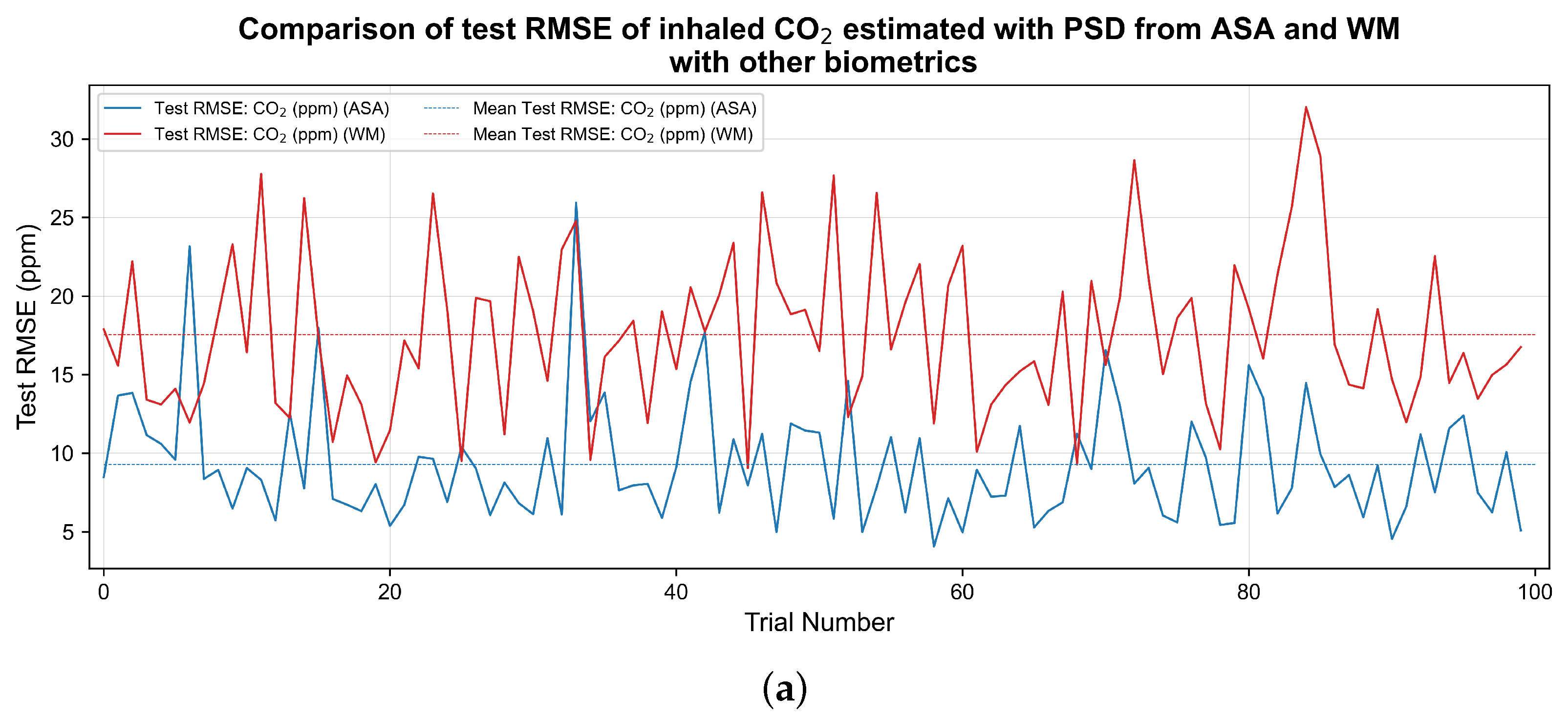
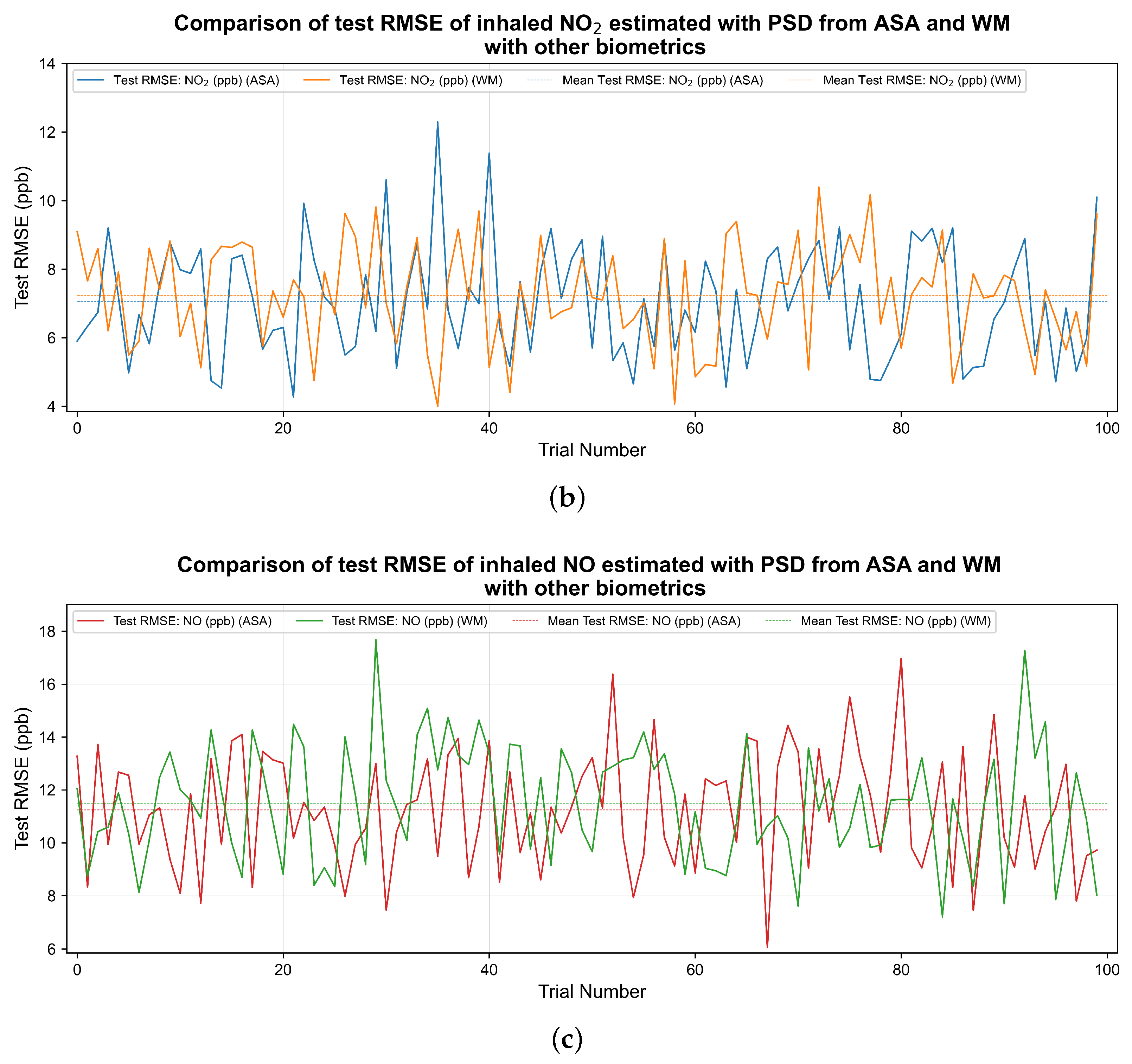
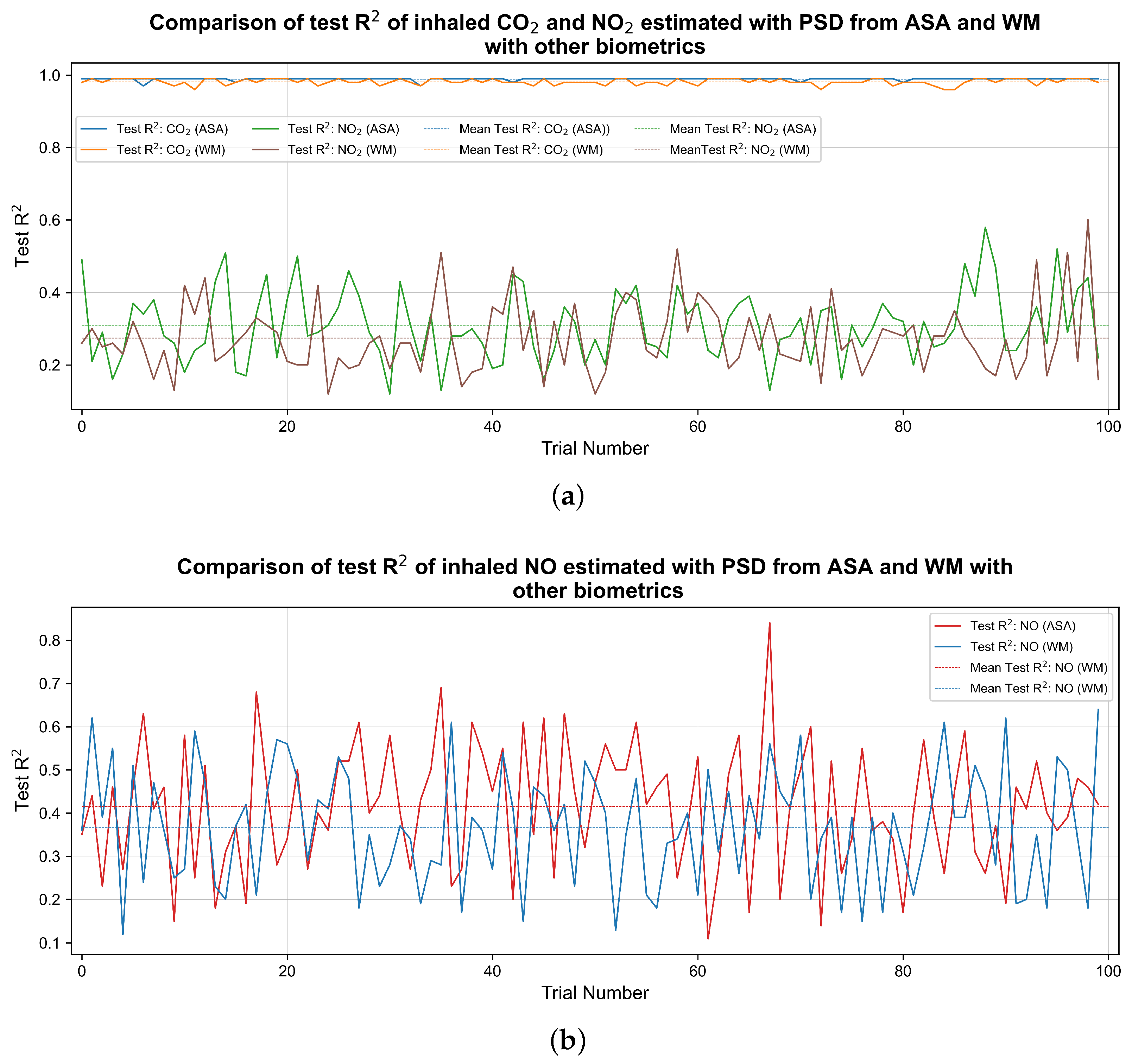
Pollutant	Average Test ${\mathrm{R}}^2$ (PSD by WM)	Average Test ${\mathrm{R}}^2$ (PSD from ASA)	Average Test RMSE (PSD by WM)	Average Test RMSE (PSD from ASA)
${\mathrm{CO}}_2$	0.98	0.98	17.55 ppm	9.28 ppm
NO	0.36	0.41	11.50 ppb	11.24 ppb
${\mathrm{NO}}_2$	0.27	0.30	7.23 ppb	7.06 ppb

shows the average ${\mathrm{R}}^2$ and average RMSE between the true and estimated values in an independent test set after running the machine learning model a total of 100 times. The input features have the same physiological responses, while the PSD is obtained either by the WM or from the ASA.

Table 3 shows that there was a significant improvement in the average RMSE value in an independent test set of ${\mathrm{CO}}_2$ when the input features were a combination of physiological responses and the PSD from the ASA, compared to when the input features were a combination of the same physiological responses and the PSD obtained by the WM. The results for the average test RMSE and average test ${\mathrm{R}}^2$ show small improvements in the case of ${\mathrm{NO}}_2$ and NO when the input features were a combination of physiological responses and the PSD from the ASA, compared to when the same physiological responses were combined with the PSD obtained by the WM.

Figure 3a shows the changes in the RMSE in an independent test for ${\mathrm{CO}}_2$ in each of the trials when the physiological responses were combined first with the PSD obtained by the WM and then with the PSD from the ASA. The figure shows that, in the majority of cases in the trial, the RMSE was smaller when the PSD from the ASA was used with other biometrics. On the other hand, Figure 3b,c shows that the results of the test RMSE in the case of ${\mathrm{NO}}_2$ and NO, respectively, exhibit a small improvement when the physiological responses were combined with the PSD from the ASA, compared to when the physiological responses were combined with the PSD obtained by the WM.

Similarly, Figure 4 shows the line graph of the ${\mathrm{R}}^2$ value between the true and estimated values of the pollutant in an independent test set for each of the 100 trials. Figure 4a shows that in the case of ${\mathrm{CO}}_2$, the ${\mathrm{R}}^2$ value is closer to 1 in most cases when the physiological responses were combined with the PSD from the ASA compared with when they were combined with the PSD obtained by the WM. Similarly, a small improvement in test ${\mathrm{R}}^2$ can also be seen in the case of ${\mathrm{NO}}_2$ and NO, as shown in Figure 4a and Figure 4b, respectively.

A scatter plot of an instance among the 100 trials for each of the pollutants is shown in Figure 5. On the left, we have the scatter diagram for when the input features were a combination of the physiological responses and the PSD from the ASA for each pollutant: (a) ${\mathrm{CO}}_2$, (c) NO, and (e) ${\mathrm{NO}}_2$. On the right, the input features were a combination of the physiological responses and the PSD obtained by the WM for each pollutant: (b) ${\mathrm{CO}}_2$, (d) NO, and (f) ${\mathrm{NO}}_2$. The curves above and to the right of these scatter plots indicate the density curves of the data points for the true values and estimated values, respectively. In each of these figures, the training data are represented by blue circles, while the testing data are represented by orange circles. Given the improvements in estimation when the physiological responses were combined with the PSD from the ASA—compared with the estimation obtained using the same physiological responses combined with the PSD obtained by the WM—the data points on the left are closer to the 1:1 line than to the 1:1 line on the right. This is clearly visible for ${\mathrm{CO}}_2$, as a significant improvement in the average test RMSE value was obtained in this case when compared to the case of ${\mathrm{NO}}_2$ and NO. In the case of ${\mathrm{NO}}_2$ and NO, the scatter plots for both cases are similar, as the improvements in these two cases were found to be small. This is indicated by the ${\mathrm{R}}^2$ and RMSE between the true and estimated values for these pollutants in their corresponding figures. The estimation for these two pollutants, however, seems to be good for small values of the pollutants, whereas the points tend to deviate from their corresponding 1:1 line as the values increase, as shown in Figure 5c–f.

An instance of the quantile–quantile plot among the 100 trials is shown in Figure 6. On the left is the quantile–quantile plot when the physiological responses combined with the PSD from the ASA were used in the case of (a) ${\mathrm{CO}}_2$, (c) NO, and (e) ${\mathrm{NO}}_2$. On the right, the plots show the quantile–quantile plot when the same physiological responses were combined with the PSD obtained by the WM in the case of (b) ${\mathrm{CO}}_2$, (d) NO, and (f) ${\mathrm{NO}}_2$. In each of these figures, the training data are represented by blue circles, whereas the testing data are represented by orange “x” signs. It can be seen in Figure 6a that the quantiles are closer to the 1:1 line for most of the distribution in both the training and the testing set as compared to Figure 6b. This indicates better prediction when the physiological responses were combined with the PSD from the ASA when compared with the physiological responses combined with the PSD obtained by the WM. The quantiles also tend to deviate from the 1:1 line when the concentration of ${\mathrm{CO}}_2$ is between 700–800 ppm. In the case of ${\mathrm{NO}}_2$ and NO, as shown in Figure 6c–f, the quantile–quantile plots indicate that the distribution is closer to the 1:1 line for smaller values of the pollutants, whereas the points tend to deviate for larger values. Furthermore, as the estimation of these pollutants was similar when physiological responses were combined with the PSD from the ASA when compared with the physiological responses combined with the PSD obtained by the WM, the structure of these quantile-quantile plots is also similar.

In the process of estimating inhaled concentrations of ${\mathrm{CO}}_2$, ${\mathrm{NO}}_2$, and NO, we used a large number of input variables—specifically, 328. As mentioned in Section 2.3, in order to identify the importance of the features, a SHAP value summary plot was plotted, as shown in Figure 7. The bar graphs are arranged in descending order such that the feature with the highest importance is at the top. Since the number of input features are high, the ranking of the variables, especially when the SHAP values are close, can vary when the data are shuffled, whereas the ranking of the variables at the top remain consistent, as their SHAP values are higher compared to the other variables. Figure 7a,c,e show the feature importance plots when the physiological responses were combined with the PSD from the ASA, whereas the figures on the right (Figure 7b,d,f) show the feature importance plots when the same physiological responses were combined with the PSD obtained by the WM. Each of the feature importance plots shows that responses such as average pupil diameter, GSR, skin temperature, respiration rate, and ECG are common in the majority of cases.

A small number of the EEG electrodes and their corresponding bands also seem to appear in some cases. The electrodes with even and those with odd numbers after the letters are located on the right side and left side of the brain, respectively [20]. The FT electrode variable, as shown in Figure 7a,c, is located between the frontal and temporal lobe; the T7 electrode variable, as shown in Figure 7b, is located on the temporal lobe on the left side of the brain; the P8 electrode variable, as shown in Figure 7e, is located in the parietal lobe on the right side of the brain.

4. Discussion

The human body responds to a lot of factors, such as temperature, altitude, humidity, air quality, external light, and several other environmental variables. The underlying principle that in this study and our previous study [17,18] was to use the autonomous responses (or biometrics) in the human body that result from the intake of pollutants in the air. Our results show that these autonomous responses can be used to estimate the inhaled concentrations of ${\mathrm{CO}}_2$ and PM [17], with high precision when using machine learning regression. The basis of all these studies is to use the body as a sensor.

The main contribution of this study is the introduction of the Astropi Spectrum Analyzer (ASA), which is a novel approach to converting the time series of electrical activity in the brain measured using EEG into a power spectrum density of various bands. We used physiological responses and a PSD from the ASA as well as a PSD obtained by the WM to estimate the inhaled concentration sof ${\mathrm{CO}}_2$, ${\mathrm{NO}}_2$, and NO. The results in Table 2 show that combining the physiological responses with the PSD from the ASA provides significant improvements in the estimation of ${\mathrm{CO}}_2$, as indicated by the average RMSE in a test set of 9.28 ppm. This is in comparison with the estimation made using the same physiological responses combined with the PSD obtained by the WM, as indicated by an average RMSE in an independent test of 17.55 ppm after running the machine learning model 100 times. For this study, we considered running 100 trials to be sufficient given the number of records we have. These improvements can also be seen by comparing the scatter diagrams in Figure 5a,b and also by comparing the quantile–quantile plots in Figure 6a,b, where the values are closer to their corresponding 1:1 line when the input variables considered were a combination of the physiological responses with the PSD from the ASA rather than a combination of the physiological responses with the PSD obtained by the WM.

However, the improvements in the results of the estimation of inhaled ${\mathrm{NO}}_2$ and NO were found to be small. One possible reason for the small improvement could be due to the EEG PSD having small SHAP values or a small contribution to the estimation of ${\mathrm{NO}}_2$ and NO. This is shown in Figure 7c,e, which shows the SHAP summary plots for ${\mathrm{NO}}_2$ and NO, respectively. Each of these figures show that there is only a single feature from the EEG PSD that ranks among the top nine features that contributed to estimating these pollutants. Since the contribution of the EEG PSD for these pollutants is small, the improvements in the results were also small.

The results for the estimation of ${\mathrm{NO}}_2$ and NO are also not as highly accurate as those for the estimation of ${\mathrm{CO}}_2$ and PM. As we hypothesized previously [17,18], the autonomous responses were most likely dominated by the inhalation of PM and ${\mathrm{CO}}_2$, due to which the estimation of these two pollutants was found to be high when compared to the estimation of ${\mathrm{NO}}_2$ and NO. The results for ${\mathrm{NO}}_2$ and NO, however, accurately display their smaller values, as indicated by the scatter diagram in Figure 5c–f and the quantile–quantile plot in Figure 6c–f. We predict that the collection of large quantities of data for these two pollutants could improve prediction accuracy and enable the machine learning model to learn from a wide range of training data and then be tested on an independent test set. This can also be seen in the same scatter diagram and the quantile–quantile plot, where the data points deviate from their corresponding 1:1 line as they become scarce for higher values of their pollutants.

This study has two key limitations: First, the limited dataset, which can be rectified by the collection of large quantities of data; this can be achieved by increasing the data collection time. Second, the use of a single participant limits the generalizability of the findings. Furthermore, the autonomous responses of the human body, such as skin temperature and sweat response, resulting from the inhalation of these pollutants vary between individuals. While multiple trials were conducted at different locations during data collection, future studies could include multiple participants from diverse demographic backgrounds to provide a broader dataset. This would ensure that a machine learning regression model would have enough representative data points to enhance the generalizability of the study.

It should be noted that improvements in the estimation of inhaled concentrations of ${\mathrm{CO}}_2$ were achieved, despite the fact that only a few features of the EEG PSD obtained using the ASA made the biggest contribution to the estimation of the pollutant, as shown in Figure 7a. It is reasonable to expect that the relative advantage of the ASA will be even greater for applications that are more purely based on spectral data, which remain a topic for future research.

References

- WHO. What Are the WHO Air Quality Guidelines? 2024. Available online: https://www.who.int/news-room/feature-stories/detail/what-are-the-who-air-quality-guidelines (accessed on 12 November 2024).
- Environmenal Protection Agency. Reviewing National Ambient Air Quality Standards (NAAQS): Scientific and Technical Information. 2024. Available online: https://www.epa.gov/naaqs (accessed on 12 November 2024).
- Hutter, H.P.; Haluza, D.; Piegler, K.; Hohenblum, P.; Fröhlich, M.; Scharf, S.; Uhl, M.; Damberger, B.; Tappler, P.; Kundi, M.; et al. Semivolatile compounds in schools and their influence on cognitive performance of children. Int. J. Occup. Med. Environ. Health 2013, 26, 628–635. [Google Scholar]
- Satish, U.; Mendell, M.J.; Shekhar, K.; Hotchi, T.; Sullivan, D.; Streufert, S.; Fisk, W.J. Is CO2 an indoor pollutant? Direct effects of low-to-moderate CO2 concentrations on human decision-making performance. Environ. Health Perspect. 2012, 120, 1671–1677. [Google Scholar] [CrossRef]
- Zhang, X.; Zhang, T.; Luo, G.; Sun, J.; Zhao, C.; Xie, J.; Liu, J.; Zhang, N. Effects of exposure to carbon dioxide and human bioeffluents on sleep quality and physiological responses. Build. Environ. 2023, 238, 110382. [Google Scholar] [CrossRef]
- Zhang, X.; Wargocki, P.; Lian, Z. Physiological responses during exposure to carbon dioxide and bioeffluents at levels typically occurring indoors. Indoor Air 2017, 27, 65–77. [Google Scholar] [PubMed]
- Jin, R.N.; Inada, H.; Négyesi, J.; Ito, D.; Nagatomi, R. Carbon dioxide effects on daytime sleepiness and EEG signal: A combinational approach using classical frequentist and Bayesian analyses. Indoor Air 2022, 32, e13055. [Google Scholar]
- Xu, F.; Uh, J.; Brier, M.R.; John Hart, J.; Yezhuvath, U.S.; Gu, H.; Yang, Y.; Lu, H. The Influence of Carbon Dioxide on Brain Activity and Metabolism in Conscious Humans. J. Cereb. Blood Flow Metab. 2011, 31, 58–67. [Google Scholar] [CrossRef] [PubMed]
- Gillespie-Bennett, J.; Pierse, N.; Wickens, K.; Crane, J.; Howden-Chapman, P. The respiratory health effects of nitrogen dioxide in children with asthma. Eur. Respir. J. 2011, 38, 303–309. [Google Scholar] [CrossRef]
- Cibella, F.; Cuttitta, G.; Della Maggiore, R.; Ruggieri, S.; Panunzi, S.; De Gaetano, A.; Bucchieri, S.; Drago, G.; Melis, M.R.; La Grutta, S.; et al. Effect of indoor nitrogen dioxide on lung function in urban environment. Environ. Res. 2015, 138, 8–16. [Google Scholar] [CrossRef]
- Latza, U.; Gerdes, S.; Baur, X. Effects of nitrogen dioxide on human health: Systematic review of experimental and epidemiological studies conducted between 2002 and 2006. Int. J. Hyg. Environ. Health 2009, 212, 271–287. [Google Scholar] [CrossRef]
- Huang, S.; Li, H.; Wang, M.; Qian, Y.; Steenland, K.; Caudle, W.M.; Liu, Y.; Sarnat, J.; Papatheodorou, S.; Shi, L. Long-term exposure to nitrogen dioxide and mortality: A systematic review and meta-analysis. Sci. Total Environ. 2021, 776, 145968. [Google Scholar] [CrossRef]
- Crüts, B.; van Etten, L.; Törnqvist, H.; Blomberg, A.; Sandström, T.; Mills, N.L.; Borm, P.J. Exposure to diesel exhaust induces changes in EEG in human volunteers. Part. Fibre Toxicol. 2008, 5, 4. [Google Scholar]
- Witek, J.; Lakhkar, A.D. Nitric Oxide. In StatPearls; StatPearls Publishing: Treasure Island, FL, USA, 2024. [Google Scholar]
- Weinberger, B. The Toxicology of Inhaled Nitric Oxide. Toxicol. Sci. 2001, 59, 5–16. [Google Scholar] [CrossRef]
- Miller, O.; Celermajer, D.; Deanfield, J.; Macrae, D. Guidelines for the safe administration of inhaled nitric oxide. Arch. Dis. Child. Fetal Neonatal Ed. 1994, 70, F47. [Google Scholar] [CrossRef] [PubMed]
- Talebi, S.; Lary, D.J.; Wijeratne, L.O.; Fernando, B.; Lary, T.; Lary, M.; Sadler, J.; Sridhar, A.; Waczak, J.; Aker, A.; et al. Decoding physical and cognitive impacts of particulate matter concentrations at ultra-fine scales. Sensors 2022, 22, 4240. [Google Scholar] [CrossRef]
- Ruwali, S.; Talebi, S.; Fernando, A.; Wijeratne, L.O.; Waczak, J.; Dewage, P.M.; Lary, D.J.; Sadler, J.; Lary, T.; Lary, M.; et al. Quantifying Inhaled Concentrations of Particulate Matter, Carbon Dioxide, Nitrogen Dioxide, and Nitric Oxide Using Observed Biometric Responses with Machine Learning. BioMedInformatics 2024, 4, 1019–1046. [Google Scholar] [CrossRef]
- Welch, P. The use of fast Fourier transform for the estimation of power spectra: A method based on time averaging over short, modified periodograms. IEEE Trans. Audio Electroacoust. 1967, 15, 70–73. [Google Scholar] [CrossRef]
- Acharya, J.N.; Hani, A.J.; Cheek, J.; Thirumala, P.; Tsuchida, T.N. American clinical neurophysiology society guideline 2: Guidelines for standard electrode position nomenclature. Neurodiagnostic J. 2016, 56, 245–252. [Google Scholar]
- Breiman, L. Random forests. Mach. Learn. 2001, 45, 5–32. [Google Scholar]
- Pedregosa, F.; Varoquaux, G.; Gramfort, A.; Michel, V.; Thirion, B.; Grisel, O.; Blondel, M.; Prettenhofer, P.; Weiss, R.; Dubourg, V.; et al. Scikit-learn: Machine Learning in Python. J. Mach. Learn. Res. 2011, 12, 2825–2830. [Google Scholar]
- Grinsztajn, L.; Oyallon, E.; Varoquaux, G. Why do tree-based models still outperform deep learning on typical tabular data? In Proceedings of the Thirty-sixth Conference on Neural Information Processing Systems Datasets and Benchmarks Track, New Orleans, LA, USA, 28 November–9 December 2022. [Google Scholar]
- Shwartz-Ziv, R.; Armon, A. Tabular Data: Deep Learning is Not All You Need. arXiv 2021, arXiv:2106.03253. [Google Scholar]
- Lundberg, S.M.; Lee, S.I. A Unified Approach to Interpreting Model Predictions. In Proceedings of the Advances in Neural Information Processing Systems, Long Beach, CA, USA, 4–9 December 2017; Guyon, I., Luxburg, U.V., Bengio, S., Wallach, H., Fergus, R., Vishwanathan, S., Garnett, R., Eds.; Curran Associates, Inc.: Brooklyn, NY, USA, 2017; Volume 30. [Google Scholar]
- Lundberg, S.M.; Erion, G.; Chen, H.; DeGrave, A.; Prutkin, J.M.; Nair, B.; Katz, R.; Himmelfarb, J.; Bansal, N.; Lee, S.I. From local explanations to global understanding with explainable AI for trees. Nat. Mach. Intell. 2020, 2, 2522–5839. [Google Scholar]