Comparison of Different Modeling Techniques for Flemish Twitter Sentiment Analysis

Abstract

Microblogging websites such as Twitter have caused sentiment analysis research to increase in popularity over the last several decades. However, most studies focus on the English language, which leaves other languages underrepresented. Therefore, in this paper, we compare several modeling techniques for sentiment analysis using a new dataset containing Flemish tweets. The key contribution of our paper lies in its innovative experimental design: we compared different preprocessing techniques and vector representations to find the best-performing combination for a Flemish dataset. We compared models belonging to four different categories: lexicon-based methods, traditional machine-learning models, neural networks, and attention-based models. We found that more preprocessing leads to better results, but the best-performing vector representation approach depends on the model applied. Moreover, an immense gap was observed between the performances of the lexicon-based approaches and those of the other models. The traditional machine learning approaches and the neural networks produced similar results, but the attention-based model was the best-performing technique. Nevertheless, a tradeoff should be made between computational expenses and performance gains.

1. Introduction

In recent decades, social media has boomed immensely. The total number of social media users has more than tripled since 2010. More specifically, it is estimated that the total number of social media users increased from 0.97 billion in 2010 to 4.2 billion, and the total is expected to increase further in subsequent years. In this social media landscape, Twitter possesses more than 370 million users, and each day, more than 500 million tweets are sent out to the world [1]. Therefore, Twitter sits on a substantial amount of data that are valuable for all kinds of research (for example, sentiment analysis).

Sentiment analysis is the research field that tries to detect people’s sentiments, opinions, emotions, etc., in a written text [2]. This research field has been widely studied over the last two decades. The authors of [3] named the year 2001 or so as the start of the large-scale awareness of the research problems in this field. Some factors that explain the increasing interest in the research challenges of sentiment analysis are the rise of machine-learning techniques and datasets that have become available through the increased usage of the Internet. Many websites where reviews and opinions concerning a certain topic can be written are available. Therefore, as stated before, social media websites such as Twitter form an excellent source of input data for sentiment analysis. However, not only social media is prone to this type of analysis; movie reviews also constitute an excellent data source [4]. Subtasks of sentiment analysis are, for example, polarity or emotion detection. More recent advances in this research field focus on aspect-based sentiment analysis [5,6] or conversational sentiment analysis [7]. These are natural language processing tasks where the sentiment of a certain aspect in the text or consecutive sentences is considered, respectively.

The key contribution of our paper lies in its innovative experimentation: f combining different existing models and techniques and using them on a Flemish dataset. First, we applied different preprocessing approaches and vector representations using a carefully chosen set of sentiment analysis techniques. More specifically, preprocessing techniques such as stemming and lemmatization were used to check whether more preprocessing would, as expected, lead to better results. Moreover, we aimed to compare models with various levels of complexity: lexicon-based methods, traditional machine-learning methods, neural networks, and attention-based models. As shown in [4], a comparison of the techniques employed by these various types of models is rare in the literature. Usually, models trained in benchmark studies belong to the same category; for example, some deep learning models may be compared with other deep learning models. However, inspired by [8], where simple models achieved strong performances, we examined whether a very advanced attention-based model is required for our dataset. In contrast, can simple techniques also result in decent sentiment analysis performance?

Moreover, we collected a new dataset containing Flemish tweets. Significantly less research has been conducted regarding sentiment analysis for the Flemish language than for English. Additionally, most studies researching natural language processing (NLP) in the Dutch language also involve training on Dutch datasets; however, Flemish, spoken in the northern part of Belgium, differs significantly from the Dutch spoken in the Netherlands, especially in an informal setting such as Twitter. The main differences between these two languages lie in the type of vocabulary used, the usage of different pronouns, and the integration of words from different languages, which is more pronounced in Flemish than in Dutch tweets. We refer the reader to Appendix A for examples of tweets in Dutch and Flemish. Another layer of difficulty is added by the fact that Flemish tweets often contain multiple languages, most often Flemish, English, and French. Therefore, this paper adds to the existing literature on sentiment analysis. To the best of our knowledge, a paper has never compared the above-mentioned techniques of varying complexity in combination with different preprocessing approaches on a dataset containing Flemish tweets. The code for this paper can be found at https://github.com/manon-reusens/Comparison-of-techniques-for-Flemish-Twitter-Sentiment-Analysis.

The paper is structured as follows. First, we discuss recent related work. Next, we describe the methodology used in this paper. Finally, we show and discuss the results of the experiments and form an overall conclusion.

2. Related Work

2.1. Benchmark Studies

Many sentiment analysis studies have been conducted. In Table 1, a compact overview of several recent studies is shown. For a complete overview of the benchmark studies in sentiment analysis, we would like to refer the reader to literature reviews or tertiary studies such as [4].

Table 1. Overview of the benchmark sentiment analysis studies.

Source	Language	Social Media Data	Sentiment	Lexicon-Based Methods	Traditional Machine Learning Models	Neural Networks	Attention-Based Models
[8]	English	✘	Polarity (Binary)	🗸	🗸	🗸	🗸
[10]	Greek	🗸	Polarity (Ternary)	✘	🗸	🗸	🗸
[11]	Saudi	🗸	Emotions	✘	🗸	✘	✘
[9]	Persian	✘	Polarity (Binary)	✘	🗸	🗸	✘
[12]	English	🗸	Polarity (Quinary)	🗸	✘	🗸	🗸
[13]	Arabic	🗸	Emotions	✘	🗸	🗸	✘
[14]	English	🗸	Polarity (Ternary)	✘	✘	🗸	🗸
Our Study	Flemish	🗸	Polarity (Ternary)	🗸	🗸	🗸	🗸

As shown in Table 1, the utilized datasets vary significantly both in language and type of data contained within them. Many languages have been considered by these different studies, though English is appears most frequently both in this table and in the literature in general. Notably, other languages have also been studied; however, the amount of literature available for English outweighs that for any other language [4]. The table also indicates the type of input data used for the benchmark analysis. In [8], movie reviews were used, and the authors of [9] used both movie reviews and hotel reviews as input data. Nevertheless, the field of sentiment analysis is not limited to the previously listed input sources; any written text can be used to conduct sentiment analysis.

A detected sentiment can be expressed as a polarity or an emotion. Polarity can be either binary (positive or negative) or ternary (positive, neutral, or negative). However, one study [12] shown in Table 1 also detected polarity with quinary target variables; a scale ranging from very negative to very positive was used. This is what the authors of [15] refer to as the assignment of the degrees of positivity or negativity in polarity analysis. This is also a very interesting field; however, as the target variable in this paper is ternary, it is out of the scope of this study. For the categorizations of emotions performed by [11,13], we would like to refer the reader to the original papers.

The last four columns in Table 1 show the types of models used in the various studies. We categorized them into lexicon-based methods, traditional machine-learning models, neural networks, and attention-based models. A lexicon-based method is a model that uses a lexicon or dictionary to detect sentiments. This lexicon is specifically created for sentiment analysis. Traditional machine-learning techniques include logistic regression, naive Bayes, and random forest. These techniques are widely used for several tasks and have existed for a long time. The next category is neural networks. This category contains several different models, such as feedforward neural networks (FFNNs), convolutional neural networks (CNNs), recurrent neural networks (RNNs), and long short-term memory (LSTM). Finally, attention-based models are approaches that, as implied by their name, use attention, such as transformers. Table 1 clearly shows that studies that benchmark models in all four distinct categories are rare. Only one of the selected benchmark studies [8] did this, yet not for social media data. More often, the tested models fall within one or two of the described categories. These results are in line with what the authors of [4] found in their tertiary study on sentiment analysis. They showed a clear overview of common approaches in this research field. Note, however, that as attention-based models are fairly newly adopted models, they were not included in their study.

For all studies mentioned in Table 1 where an attention-based model was included, this model consistently outperformed the other models. However, in our opinion, one important nuance should be noted. For example, in [8], a simple logistic regression model achieved high performance that was similar to that of a bidirectional encoder representation from a transformer (BERT) model. More specifically, the accuracy of the logistic regression model was 89.42%, and the BERT reached an accuracy of 92.31%. Even though the authors mentioned this, they neglected to stress this finding. This could suggest that for a simple problem such as sentiment analysis, the use of attention-based models might be too advanced, especially with binary predictions. Our hypothesis is also supported by [2]. In this book, Liu stated the following: In general, sentiment analysis is a semantic analysis problem, but it is highly focused and confined because a sentiment analysis system does not need to fully understand each sentence or document; it only needs to comprehend some aspects of it, for example, positive and negative opinions and their targets (Liu 2015, p. 15). Moreover, in [4], the authors mentioned that traditional machine-learning models often perform similarly to deep learning methods, and sometimes even outperform them. The authors of [15], however, contradicted this hypothesis. They stated that these traditional machine-learning models work well when given a large amount of input text. According to them, the models are not able to handle sentiment analysis at the sentence level. As tweets have a character limit, this might cause a performance decrease. After finding these conflicting views, we wanted to check which hypothesis applies to our dataset containing Flemish tweets.

2.2. Multilingual Sentiment Analysis

Besides studies researching one specific language, multilingual sentiment analysis has been studied. In [16], its authors classified this task into two categories: cross-lingual sentiment classification and multilingual sentiment classification. The first aims at training a model for a language for which no data are available. The goal of the second category is to train a model that performs well on average for all languages. In [17], its authors provide an overview of different ways to tackle both categories. Often, lexicon-based methods are used, sometimes including translating the words to one language. In other cases, such as [18], classifiers are trained on corpora of different languages to create one multilingual model. As far as we know, every input was written in one language, and thus not a mixture of languages. More recently, the authors of [19] proposed BabelSenticNet as a solution to easily generate SenticNet for various languages. This model was construction through statistical machine translation and over-mapping for increased robustness. It provides the polarity of words in 40 languages.

2.3. Preprocessing

In addition to the different modeling choices described above, several decisions have to be made regarding preprocessing. Many different possibilities exist, some of which are language-specific. Table 2 represents the most common preprocessing techniques used by the benchmark studies mentioned in Table 1.

Table 2. Overview of the utilized preprocessing methods.

Source	Punctuation	Repeated Letters	URLs	Numbers	#	@	Capital Letters	Stop Words	Emoticons
[8]	🗸	✘	✘	✘	🗸	🗸	🗸	🗸	✘
[10]	✘	✘	🗸	✘	🗸	🗸	🗸	✘	🗸
[12]	✘	✘	✘	🗸	✘	✘	✘	✘	✘
[9]	✘	🗸	✘	✘	✘	✘	✘	✘	✘
[11]	🗸	🗸	🗸	🗸	🗸	🗸	✘	🗸	🗸
[13]	✘	🗸	✘	🗸	✘	✘	✘	🗸	🗸
[14]	✘	🗸	🗸	🗸	🗸	🗸	🗸	✘	🗸
Our Study: Textified	✘	✘	🗸	✘	✘	✘	✘	✘	🗸
Our Study: Stemmed	🗸	✘	🗸	✘	🗸	🗸	🗸	🗸	🗸
Our Study: Lemmatized	🗸	✘	🗸	✘	🗸	🗸	🗸	🗸	🗸

Table 2 must be interpreted as follows. The columns represent the changes made to the input text; for example, a checkmark in punctuation refers to a change in punctuation compared to that of the original text. This can be either a modification or removal of the respective variable. As previously stated, this table contains the most frequently utilized techniques and is therefore incomplete. Other approaches include changing Arabic diacritics, changing can’t to cannot, removing accents, etc. These techniques are often language-specific and were therefore not included in our study. Another remark that must be made is that in [13], special characters were also removed. However, it was not specified what these ‘special characters’ included. Therefore, we do not indicate the removal of punctuation, #, or @ in the table.

The last three rows represent the preprocessing performed in our study. A detailed explanation is given in Section 3.2. In short, three preprocessing approaches were used in this study, and in addition to the methods described in the table, stemming and lemmatization were used in the second and third approaches, respectively. It is interesting to note that in [8], lemmatization was used, and in [9], stemming was performed. As seen, we also never removed repeated letters or numbers, since the authors of [20] concluded that both of these methods do not significantly affect performance.

2.4. Ground Truth and Annotations

Another problem that we briefly discuss is the choice of the ground truth in the dataset. Usually, human annotators are involved, and their annotations are taken as the ground truth. However, the specific retrieval processes of these annotations differ immensely across different benchmark studies. The following paragraph discusses the creation of a ground truth for the previously considered benchmark studies.

Many of the previously mentioned studies used publicly available datasets for their analyses [8,13,14,20]. Most other studies used three human annotators that manually labeled the given datasets [9,10,12]. However, the authors rarely described what happened when the annotators disagreed. Only in [12] did the authors mention that the annotations were solely accepted if all three annotators agreed or if two out of three agreed and the third annotation only differed by one from those of the other annotators (in this study, five categories were used, with zero representing very negative and five representing very positive). Otherwise, a fourth annotator was used. One of the analyzed studies collected its ground-truth sentiments differently than in the previously discussed studies. In [11], a list was composed of words for each emotional class. This list was then used to categorize the input tweets into distinct classes.

3. Methodology

3.1. Data

The dataset used in this study was obtained through Statistics Flanders. It contains 47,096 Flemish tweets, which were classified into three categories (negative, neutral, and positive) by five annotators. Each tweet was annotated by at least one annotator. If a tweet was annotated by multiple people, we decided to keep the tweet only if all annotators agreed. The Flemish tweets in this dataset were defined as Dutch tweets that were tweeted in Belgium. We decided to create our own dataset, since we wanted a dataset containing Flemish tweets, and not a dataset also containing tweets from the Netherlands. However, it should be noted that the language of Twitter is often a collection of multiple languages; for example, English and French were also represented in the dataset. Moreover, the dataset also contained some French tweets. However, we decided to leave them in as noise, since the Twitter API also did not detect them. Thus, this makes the dataset representative for future evaluations. Table 3 shows an overview of the distribution of the tweets in our dataset. This distribution was obtained by randomly sampling tweets over a period of five years (2015–2020). By choosing this approach, no specific trending topics would dominate the dataset. Therefore, this random sample provides a good representation of reality. The use of SMOTE would be beneficial when dealing with a highly imbalanced dataset, as shown in [21].

Table 3. Overview of the dataset.

Category	Number of Tweets
Positive	14,572
Negative	14,357
Neutral	18,167

3.2. Preprocessing

For our experiments, we decided to perform three types of preprocessing to compare the different approaches. We used these different types of preprocessing steps for the lexicon-based and traditional machine-learning approaches. These different approaches are illustrated on our GitHub page (https://github.com/manon-reusens/Comparison-of-techniques-for-Flemish-Twitter-Sentiment-Analysis)

We started by deleting URLs and changing emoticons to words for all tweets. This was considered the first preprocessing approach, the results of which we call textified. Next, we went further with the textified tweets to perform the two other preprocessing approaches. We deleted punctuation, hashtags (#), and at signs (@). Moreover, we changed capital letters to lowercase letters and deleted all stop words. These steps were the same for both remaining approaches. However, for one approach, we then used stemming, and for the other approach, we used lemmatization. The resulting data are said to be stemmed and lemmatized, respectively. Table 2 concisely summarizes the preprocessing steps performed in the different approaches. As represented in the table, no preprocessing regarding repeated letters or numbers was performed. This decision was based on a finding in [20]. In this paper, the influences of different preprocessing techniques on the performances of different traditional machine-learning models were checked. As seen in the paper, nearly no difference in performance was noted across the different models based on the removal of repeated letters when predicting three classes.

Next, we split the preprocessed dataset into training and test sets. Seventy percent of the dataset was used as the training set, and 30% was included in the test set. Afterward, the training set was again split into training and validation sets (80% and 20%, respectively). The validation set was used throughout the different experiments to tune the parameters of the different models. For both splits, the distribution of the data over the different classes was respected.

3.3. Models

3.3.1. Lexicon-Based Method

First, we implemented two lexicon-based approaches. This type of model utilizes a lexicon or dictionary to calculate a score. This score is then deployed to predict the corresponding sentiment. The first language-specific lexicon-based method we included is based on the Valence-Aware Dictionary and Sentiment Reasoner (VADER) method. Since the original VADER model is an English model and we worked with Flemish data, we used a multilanguage alternative proposed in [22]. The package itself translates the input text into English via a website. However, the number of requests executed within a certain timeframe is limited. Therefore, we changed the online translator to the itranslate package [23]. Once the text was translated to English, the associated score was calculated based on an English dictionary. The output then determined the probability of the tweet belonging to one of the three classes: negative, neutral, and positive. To determine the final output, we took the maximum of these scores. If the highest score was equal among different classes, we randomly took one of them. As VADER requires the intermediate step of translation, we also wanted to include another lexicon-based method to create a representative selection of techniques for this category. Therefore, the second language-specific lexicon-based method we used implemented was TextBlob. We implemented TextBlob using [24]. Moreover, recent literature [25,26,27,28] suggests that TextBlob should produce superior results to VADER.

These experiments were completed in two steps. First, two different preprocessing techniques were used, namely, textification and lemmatization. We did not use the stemmed preprocessing approach in combination with these lexicon-based methods. The reason for this lies in the effect that stemming has on text. With stemming, the stem of a word is taken regardless of whether it is a real word. However, lexicon-based methods require existing words that appear in their dictionaries. Lemmatization, on the other hand, guarantees that a word will be changed into an existing word. Therefore, only the textification approach and lemmatization were used. Second, these two preprocessing approaches were used as inputs for the lexicon-based models as described previously.

3.3.2. Traditional Machine-Learning Models

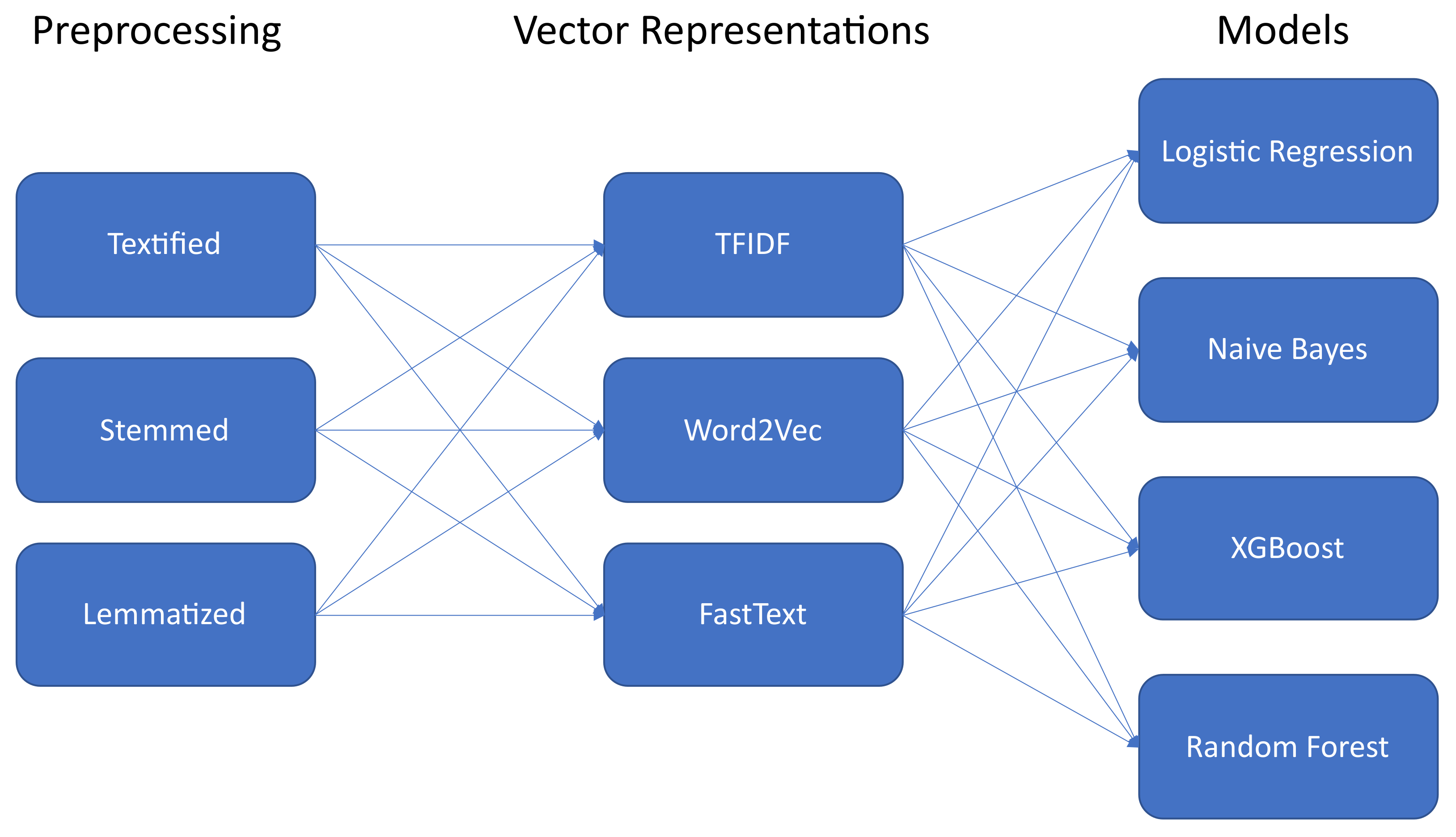
In Figure 1, an overview of the experiments conducted for the traditional machine-learning models is shown. On the left, the preprocessing techniques are depicted. For an explanation, we refer the reader to Section 3.2. After preprocessing, the sentences were transformed into vector representations. We used three types of vector representations: term-frequency inverse document-frequency (TFIDF), Word2Vec, and FastText. The tuned hyperparameters for each of these approaches are shown in Table 4.

Figure 1. Overview of experiments for the traditional machine-learning models.

Table 4. Hyperparameters tuned for each vector representation approach.

Vector Representation	Tuned Hyperparameters	Values
TFIDF	max_features n-gram range	1000, 2000, 3000, 4000, 5000, 6000, 8000, 10,000, 12,000 (1, 1), (1, 2)
Word2Vec	vector_size window min_count sg alpha	50, 100, 200, 300, 500, 600, 700, 1000 1, 2, 3, 4, 5, 6, 7, 8, 9, 10, 12, 15, 20 0, 1, 2, 3, 4, 5, 6, 7, 8, 9, 10, 20 0, 1 0.01, 0.025, 0.05, 0.1, 0.15, 0.2, 0.3, 0.4, 0.5, 0.8, 1
FastText	/	/

We implemented TFIDF by using [29]. This generated a matrix including TFIDF features, which was calculated as follows:

$$TFIDF(\mathrm{t},\mathrm{d})=TF(\mathrm{t},\mathrm{d})\times IDF\left(\mathrm{t}\right),$$

(1)

where the TF stands for the term frequency, which represents the number of times a term occurred in a certain document, and the IDF is defined as:

$$IDF\left(t\right)=log\frac{1+n}{(1+DF(t\left)\right)},$$

(2)

where DF stands for the number of documents in which the term was included. Next, the TFIDF vectors were normalized by the Euclidian norm operation.

In [30], the authors stated that TFIDF cannot fully grasp the semantic meanings of short texts, such as tweets. Therefore, we also added other approaches. We applied [31] for the implementation of Word2Vec. Pretrained Word2Vec models are available in many different languages. However, it is also possible to self-train the model. We used both approaches. The hyperparameters tuned for the self-trained model are listed in Table 4. For the pretrained model, no hyperparameters have to be tuned. Word2Vec is an algorithm that can either be trained by a skip-gram or by a continuous bag-of-words (CBOW) model. Subsequently, it learns the vector representations of words and syntactic and semantic–word relationships. The vectors encode patterns and linguistic regularities. These can often be expressed linearly—for example, vec(Queen) − vec(Woman) + vec(Man) = vec(King). Note that Word2Vec models are vector representations for words. However, we wanted a representation for an entire tweet. In [30], different techniques utilizing Word2Vec were suggested to represent sentences. One of the well-performing methods for tweets was to take the mean of the word embeddings in a tweet. Inspired by this study, we took the average of all the word representations in a sentence as the final vector representation for the corresponding tweet.

We used [32] for our pretrained Word2Vec embeddings. Most pretrained models are trained on written formal text, such as Wikipedia. In contrast, the word embeddings we used were trained on social media messages, posts from blogs, news, and fora. These pretrained embeddings were well-suited for our analysis, since our input sentences were tweets, which entailed very informal language and a different vocabulary than that of formal written texts. Note that for Word2Vec, only the textification and lemmatization preprocessing approaches were used because of the inability of stemming to guarantee existing words as outputs.

One downside of Word2Vec is that it does not try to find a corresponding vector for unknown words (i.e., it is out of vocabulary). Instead, here in our analysis, it merely generated a null vector. However, because of this disadvantage, we also decided to compare the results to those obtained when using FastText for vector representations. While taking the morphology of a word into account, this approach still tries to compute a suitable vector representation [33]. We only used pretrained word embeddings, and therefore, no hyperparameters needed to be tuned. Note that for the FastText word embeddings [34], only the textification and lemmatization preprocessing approaches were used, as above.

Next, these vector representations were used as inputs for the traditional machine-learning models. As depicted in Figure 1, four approaches were used: logistic regression, naive Bayes, extreme gradient boosting (XGBoost), and random forest. For brevity, we would like to refer the reader to [29] for more detailed explanations of logistic regression, naive Bayes, and random forest; and to [35] for XGBoost. For naive Bayes, we used two variants: multinomial naive Bayes and Bernoulli naive Bayes. In [36], the authors showed that both methods work comparably well for binary classification. Therefore, we tried out both methods for this multiclass classification task. Table 5 shows the different hyperparameters tuned for each of the models. As shown, no hyperparameters were tuned for naive Bayes, since we decided to use smoothing.

Table 5. Hyperparameters tuned for each traditional machine-learning model.

Machine Learning Model	Tuned Hyperparameters	Values
Logistic Regression	C (regularizer)	0.05, 0.1, 0.2, 0.3, 0.4, 0.5, 0.6, 0.7, 0.8, 0.9, 1
Naive Bayes	/	/
XGBoost	max_depth learning_rate n_estimators	1–10 0.01, 0.05, 0.1, 0.2, 0.5, 0.8, 1,1.2, 1.5 10, 50, 80, 100, 120, 150
Random Forest	n_estimators max_features	10, 50, 100, 150, 200 sqrt, log2

3.3.3. Neural Networks

The category of neural networks was represented by a bidirectional LSTM. The LSTM is an architecture that was first proposed in [37]. It was suggested as an improvement over RNNs to mitigate the vanishing and exploding gradient problems that could occur with this model. Moreover, an LSTM network includes an input gate, a forget gate, and an output gate. Due to this forget gate, an LSTM network can control what information is retained over a longer period of time and what information is forgotten [38].

An LSTM network, like an RNN, reads a sentence from left to right. That way, it can take the previous information in the sentence into account. However, such a network is not yet able to grasp the full meaning of a sentence, since it does not know the information that is still coming. One step in the right direction for letting LSTM understand context involves utilizing a bidirectional LSTM network. This model reads the input from left to right in one layer and from right to left in the other layer. This model was used in our study.

The tuned hyperparameters were the kernel, recurrent, bias, and activity regularizer (all tuned with the following values: $1\times {10}^{-2}$, $1\times {10}^{-3}$, $1\times {10}^{-4}$, $1\times {10}^{-5}$ and recurrent dropout parameters (both tuned by: 0.1, 0.2, 0.3). The input data were first one-hot encoded through a tokenizer, and afterward, the sequences were padded [39,40]. Our model architecture is represented in Figure 2. The padded tweets were used as inputs for the embedding layer. This layer then changed each input into a vector of length 256. This vector was then used as the input for the bidirectional LSTM layer. We used one hidden layer in our bidirectional LSTM model. This decision was based on the relative simplicity of the classification problem and the fact that the majority of the benchmark studies implemented bidirectional LSTMs with one hidden layer. The number of hidden nodes in the bidirectional LSTM model was 12. We experimented with different numbers of hidden nodes in this layer; however, we found that more hidden nodes generated similar results. Finally, the outputs of both the forward and the backward LSTM were concatenated and used as input for a final dense layer with three output nodes and a softmax activation function. This resulted in the probability of the given tweet belonging to each of the classes. The model was compiled through a categorical cross-entropy loss function, and we modified the learning rate as follows. Starting from a learning rate of $1\times {10}^{-4}$, we kept it constant for 10 epochs, and then we let it exponentially decrease until it reached $1\times {10}^{-5}$. This was subsequently used as the learning rate for the following epochs. We let our model train for 1000 epochs and executed early stopping when the accuracy on the validation set did not improve for 30 epochs. The model with the best accuracy on the validation set was saved.

Figure 2. Architecture of our bidirectional LSTM.

3.3.4. Attention-Based Model

For our study, we also trained an attention-based model. We specified a separate category for these types of models. The previous category, therefore, only included neural networks without attention. Our attention-based model was implemented by using [41]. This model is a wrapper function for the RobBERT model, a language-specific pretrained attention-based model built on RobBERTa [42]. RobBERTa is, in turn, an improved version of BERT [43]. We now explain these models in more detail.

BERT uses attention and is composed of multiple encoders. The model is usually trained in two steps. First, a pretraining step is executed, where enormous amounts of data are used to train the model in an unsupervised manner. This training procedure consists of two tasks, masked language modeling and next sentence prediction, and is intended for the model to obtain a grasp of the given language. Next, the model is fine-tuned on a task-specific dataset [44]. As stated, RobBERTa is an improved version of BERT that has some modifications, e.g., utilizing dynamic masking instead of static masking [43]. This model architecture was used in [42] and pretrained on Dutch datasets to create RobBERT.

Regarding the inputs for our model, we only used the Textified approach. We did this because in the model used, a language-specific tokenizer was already included. We used the pretrained RobBERT model and further fine-tuned it by first training the last layer of the model and the classification head. In this way, the model became familiar with the Twitter language represented in the dataset. Finally, we trained the classification head once more, while keeping all other parameters frozen. We also experimented with other training settings, but we obtained similar results.

3.4. Performance Measures

Four different performance measures were used in our study: accuracy, macro F1-score (this approach takes the mean of the metrics calculated for each label), macro precision, and macro recall.

4. Results

We now separately discuss the results obtained by each type of underlying model. Then, we combine the best results of each type and compare the best models across the different types.

4.1. Lexicon-Based Method

In Table 6, the results are shown for the two lexicon-based models. Both models were trained on the textified and lemmatized (preprocessed) sentences, indicated in the table with T and L, respectively. This table shows that for both lexicon-based methods, the lemmatized sentences outperformed the textified sentences in terms of all performance measures, except for precision. Moreover, the table indicates that the performance of TextBlob surpassed that of VADER in all measures, except for precision. However, note that with accuracies of approximately 40%, all models scored relatively poorly.

Table 6. Lexicon-based methods’ results.

Model		Accuracy	Macro F1-Measure	Macro Precision	Macro Recall
VADER	T	0.4067	0.2516	0.5584	0.3586
	L	0.4283	0.3215	0.5198	0.387
TextBlob	T	0.4241	0.3190	0.4899	0.3838
	L	0.4328	0.3234	0.5482	0.3921

4.2. Traditional Machine-Learning Models

As we used an extensive set of traditional machine learning algorithms, we give only a summary of the most remarkable findings and refer the reader to Appendix B for the details regarding all the experiments.

In general, we can conclude that for all models, the self-trained Word2Vec data were substantially worse than the other vector representations, except for XGBoost. For this ensemble method, this particular vector representation resulted in a similar performance as with TFIDF. Moreover, using TFIDF to get vector representations showed the most consistent performance for all different traditional machine-learning models. With four of the used models, it was the best-performing approach. Only for XGBoost did using pretrained Word2Vec for vector representations result in higher performance. The naive Bayes models observably did not work well with word embeddings (pretrained or self-trained). Both methods led to approximately 10% performance decreases compared to that of TFIDF. The other models achieved good performances when applying Word2Vec, and most of the time, these results were superior than when using FastText as the embedding method. Furthermore, when zooming in on the different preprocessing approaches, more preprocessing seems to lead to better results. Only in a few cases was the opposite observed, namely, for both naive Bayes models combined with the self-trained Word2Vec approach and for the pretrained word embeddings in combination with multinomial naive Bayes. Nevertheless, these performance differences were relatively small.

In Table 7, a comparison between the best-performing models among all the traditional machine-learning models is given. In terms of all performance measures, the logistic regression performed best. However, all traditional machine-learning models had similar performances. The difference from the logistic regression was always around or less than 0.5%.

Table 7. Results of the best traditional machine-learning models.

Model	Accuracy	Macro F1-Measure	Macro Precision	Macro Recall
Logistic Regression	0.6091	0.6030	0.6114	0.6012
Multinomial naive Bayes	0.6041	0.5957	0.6084	0.5956
Bernoulli naive Bayes	0.6037	0.5976	0.6021	0.5968
XGBoost	0.6030	0.5938	0.6022	0.5942
Random Forest	0.6012	0.5928	0.6053	0.5908

4.3. Neural Networks

The results of the bidirectional LSTM model are shown in Table 8. For this model, all performance measures were close to 60%. In Section 5, this is discussed further, and the results are compared with those of the other models.

Table 8. Results of the bidirectional LSTM and attention-based model.

Model	Accuracy	Macro F1-Measure	Macro Precision	Macro Recall
Bidirectional LSTM	0.6053	0.5985	0.6024	0.5986
Fine-tuned RobBERT	0.6559	0.6507	0.6537	0.6507

4.4. Attention-Based Model

Finally, the attention-based model is represented in Table 8. Approximately 65% was achieved in terms of all performance measures. This model is also discussed further in the next section.

5. Discussion

A summary of the best models by category is shown in Table 9. Among the lexicon-based methods, TextBlob employing the Lemmatized preprocessing approach yielded the best results in terms of accuracy, recall, and the F1-score, as depicted in Table 6. Therefore, we used this model to represent the lexicon-based approaches in our comparative analysis among the different categories. Regarding the traditional machine-learning models, we included the logistic regression model with TFIDF employing the Lemmatized preprocessing approach. The neural networks and attention-based models are represented by the bidirectional LSTM and fine-tuned BERT models, respectively. Table 9 shows three groups of models in terms of performance. First, TextBlob undoubtedly performed substantially worse than the other models. Second, it is noticeable that the fine-tuned RobBERT model outperformed all other models. Finally, the bidirectional LSTM and logistic regression achieved similar performances. Moreover, the traditional machine-learning model performed slightly better than the bidirectional LSTM model, even after extensively tuning the hyperparameters of this model. More advanced tuning is required to try and produce a better performance with this model; however, despite tuning being a very laborious task, it still does not guarantee that the model will then outperform logistic regression. Therefore, it is worth asking whether this possible slight performance increase justifies the extra computational power. Consequently, we conclude that the performance of the logistic regression model, which is a simpler model than the bidirectional LSTM model, was already relatively high and approached the performance of these very advanced models.

Table 9. Overview of the performance of the best model in each category.

Model	Accuracy	Macro F1-Measure	Macro Precision	Macro Recall
TextBlob	0.4328	0.3234	0.5482	0.3921
Logistic Regression	0.6091	0.6030	0.6114	0.6012
Bidirectional LSTM	0.6053	0.5985	0.6024	0.5986
Fine-tuned RobBERT	0.6559	0.6507	0.6537	0.6507

The fine-tuned RobBERT model definitely outperformed all other models trained in this study. However, this model is so complex that a tradeoff should be made between performance and computational power. Not only should the computational expenses incurred during training be considered in this tradeoff, but the model’s maintenance required when deploying it for specific applications should also be considered. Therefore, it is not necessarily always the best model to use. When considering these additional aspects, logistic regression might be preferred over the advanced models, despite its possibly poorer performance.

We would also like to shed some more light on the performances of the different preprocessing techniques and the vector representations. First, when comparing the preprocessing techniques in lights of the different models (VADER, TextBlob, logistic regression, multinomial naive Bayes, Bernoulli naive Bayes, XGBoost, and random forest), more preprocessing often led to better performance. However, as discussed previously, this was not always the case; e.g., take the Bernoulli or multinomial naive Bayes model employing self-trained Word2Vec vector representations. Moreover, more preprocessing only yielded a relatively small increase in performance which was not as pronounced as expected. Furthermore, we can look at the comparison between the stemming and lemmatization approaches. For the logistic regression, multinomial naive Bayes, and random forest models, we can see that lemmatization outperformed stemming. However, the Bernoulli naive Bayes and XGBoost models produced the opposite result. Still, the difference in these performance measures was not large for any of the models. Therefore, we can conclude that they achieved similar performance.

Second, when looking at the different vector representations, it is notable that TFIDF consistently performed well for all models. The other models, however, exhibited more performance variations. Unsurprisingly, the self-trained vector representations were often outperformed by the pretrained representations. Regarding Word2Vec and FastText, the results showed that most of the time, FastText performed slightly worse than Word2Vec. Various explanations could possibly describe this phenomenon. First, this result may have been caused by the training data used to make both pretrained models. As stated, the pretrained Word2Vec embeddings used different sources, including social media data. The FastText approach, on the other hand, used Wikipedia and Common Crawl as training data. Common Crawl is a nonprofit company that crawls the web and then makes the obtained data publicly available [34]. It is possible that because our Word2Vec embeddings put more stress on the informal language, these models performed better than those utilizing FastText. Second, it is also possible that Word2Vec might have achieved better performance because it always used zero vectors for unknown words. This would contradict our earlier assumption. The reason for adding FastText was that this model still tried to produce reasonable word vectors for unknown words, whereas Word2Vec only used null vectors.

Moreover, some threats to validity have to be discussed. Flemish is grammatically similar to English, and no different letters are used. However, Flemish sometimes uses accents on letters; therefore, we did not remove them during preprocessing. Nevertheless, the main threat to validity is the fact that Flemish tweets often contain multiple languages. When using TFIDF, this does not cause a real issue. However, when one uses word embeddings trained on corpora written in standard Dutch, this will cause problems. That could also explain why TFIDF consistently worked well for all models and pretrained word embeddings sometimes had some difficulties. In future research, we want to zoom in on this and try to mitigate this threat further by using multilingual word embeddings. Other language-specific preprocessing techniques can be looked into further too. Additionally, a more in-depth analysis of the models’ confidence can be conducted for certain predictions, as this might greatly affect further generalization on new datasets. Other interesting research opportunities lie in the combination of this research field with anomaly detection. When looking more in-depth at the different phenomena in the dataset, anomaly detection could be used to further clean the dataset and ensure that only the Flemish phenomena are incorporated into the dataset. Moreover, the combination of preprocessing steps with neural networks and the effects of these steps on the performance of the models would be interesting research to explore future. Finally, further research into the usage of dimensionality reduction techniques can be done.

6. Conclusions

The availability of opinionated texts on microblogging websites such as Twitter has significantly increased over the last few decades. Consequently, numerous studies have been conducted in the field of sentiment analysis. However, most research focuses on the English language. In this study, we compared a variety of models on a new dataset containing Flemish tweets. The novelty of our study lies in its unique experimental design: we combined several models with different preprocessing techniques and utilized various vector representations on a new Flemish dataset. More specifically, we compared lexicon-based methods, traditional machine learning approaches, neural networks, and an attention-based model. In terms of preprocessing, we studied the effects of different preprocessing methods. Finally, regarding vector representations, TFIDF, Word2Vec, and FastText were used.

In terms of preprocessing, we concluded that generally, more preprocessing led to better results, as expected. Moreover, when comparing stemming and lemmatization, the best approach depended on the underlying traditional machine-learning model. For logistic regression, multinomial naive Bayes, and random forest, lemmatization was preferable; in contrast, Bernoulli naive Bayes and XGBoost models performed best in combination with the stemming preprocessing method. However, despite this slight performance difference, both approaches led to similar results. In terms of vector representations, we noticed that TFIDF performed well in combination with every model. Only XGBoost preferred pretrained Word2Vec vector representations. Moreover, the naive Bayes models did not work well with Word2Vec or FastText word embeddings.

Finally, we conclude that the lexicon-based method did not work well at all; it only performed slightly better than a random model. The other models, however, did result in good performance. Different traditional machine learning approaches yielded similar results. In terms of accuracy and precision, the logistic regression model utilizing TFIDF after Lemmatized preprocessing was preferred. The LSTM approach produced similar, and in this case slightly worse, results than those of the best-performing traditional machine-learning models. The attention-based model undoubtedly outperformed all other models, providing an accuracy increase of more than 4% over that of the second-best model (logistic regression). Nevertheless, the attention-based model is very computationally expensive both during training and in terms of maintenance. While a logistic regression model takes minutes to train, a BERT-based model needs hours. Therefore, we do not conclude that the attention-based method is recommended for every application. The simpler models, such as the logistic regression, produced only slightly lower results. Therefore, before deploying this attention-based model, a tradeoff must be made between computational expenses and performance gains.